Calibrating High-Precision Faraday Rotation Measurements for LOFAR and the Next Generation of Low-Frequency Radio Telescopes

Faraday rotation measurements using the current and next generation of low-frequency radio telescopes will provide a powerful probe of astronomical magnetic fields. However, achieving the full potential of these measurements requires accurate removal of the time-variable ionospheric Faraday rotation contribution. We present ionFR, a code that calculates the amount of ionospheric Faraday rotation for a specific epoch, geographic location, and line-of-sight. ionFR uses a number of publicly available, GPS-derived total electron content maps and the most recent release of the International Geomagnetic Reference Field. We describe applications of this code for the calibration of radio polarimetric observations, and demonstrate the high accuracy of its modeled ionospheric Faraday rotations using LOFAR pulsar observations. These show that we can accurately determine some of the highest-precision pulsar rotation measures ever achieved. Precision rotation measures can be used to monitor rotation measure variations — either intrinsic or due to the changing line-of-sight through the interstellar medium. This calibration is particularly important for nearby sources, where the ionosphere can contribute a significant fraction of the observed rotation measure. We also discuss planned improvements to ionFR, as well as the importance of ionospheric Faraday rotation calibration for the emerging generation of low-frequency radio telescopes, such as the SKA and its pathfinders.

1 Introduction

In recent years, low-frequency ($\nu_{\rm obs}<300$ MHz) radio astronomy has undergone a revival due to the construction of the Giant Metrewave Radio Telescope (Swarup, 1991, GMRT;) and modern aperture array radio telescopes such as the LOw Frequency ARray (LOFAR; Stappers et al. 2011; van Haarlem et al. 2013, submitted), the Long-Wavelength Array (Kassim et al., 2010, LWA;), and the Murchison Widefield Array (Mitchell et al., 2010, MWA;). The first phase of the Square Kilometre Array (Garrett et al., 2010, SKA;) is also planned to feature a large number of low-frequency antennas, operating at $\sim 70-450$ MHz. These telescopes open new scientific horizons in the area of low-frequency radio astronomy, including the determination of high-precision Faraday rotation measures (RMs).

Faraday rotation causes the intrinsic polarization angle ($\chi_{\mathrm{0}}$) of a signal to rotate as it propagates through a magneto-ionic medium. The observed polarization angle of a point source can be defined as:

$$\chi=\chi_{\mathrm{0}}+(\phi_{\mathrm{ion}}+\phi_{\mathrm{ISM}}+\phi_{\mathrm{IGM}})\lambda^{\mathrm{2}},$$ (1)

where $\chi$ denotes the observed polarization angle in radians and $\lambda$ the observing wavelength in meters. $\phi$ is the Faraday depth in rad m^-2 of a given intervening magneto-ionic medium. In Eq. 1 three intervening media produce Faraday rotation: the ionosphere (ion), the Galactic interstellar medium (ISM), and the inter-galactic medium (IGM; assuming the source is extra-Galactic). Low-frequency observations are particularly affected because Faraday rotation increases quadratically with wavelength.

For the case of a single polarized source positioned behind one or more magneto-ionic media that are not emitting polarised radiation, the Faraday depth of the source is equivalent to its RM (Sokoloff et al., 1998, e.g.,). Nonetheless, here we will use the more generic term Faraday depth. Following Brentjens & de Bruyn (2005) we define Faraday depth as:

$$\phi(\@vec{\mathrm{l}})=0.81\int^{\mathrm{observer}}_{\mathrm{source}}n_{\mathrm{e}}\@vec{\mathrm{B}}\cdot\mathrm{d}\@vec{\mathrm{l}}\,\mathrm{rad}\,\mathrm{m}^{\mathrm{-2}},$$ (2)

where $n_{\mathrm{e}}$ and $\@vec{\mathrm{B}}$ are the electron density (cm^-3) and magnetic field ($\upmu$G) integrated along the line-of-sight (LOS) to the source and d$\@vec{\mathrm{l}}$ is the infinitesimal path length in pc. A magnetic field pointing towards/away from the observer gives a positive/negative Faraday depth.

The electron density in the ionosphere dictates the lowest frequency observable from the ground, approximately 10 MHz. Above this frequency, the ionosphere affects signals in three main ways: i) differential phase delays, ii) Faraday rotation, and iii) absorption in the High Frequency band (HF; 3$-$30 MHz) and the low-end of the Very High Frequency band (VHF; 30$-$300 MHz) due to the presence of the so-called “D-region” in the daytime. Assuming a typical observing frequency of 150 MHz (LOFAR high band) and an ionospheric Faraday depth of 1 rad m^-2, the additional rotation of the polarization angle imparted by the ionosphere will be $\sim 228.9^{\circ}$. Although the rotation of the polarization angle is less pronounced at higher frequencies, the Faraday depth of the source will still be systematically affected by the ionosphere. Due to the direction of the geomagnetic field, ionospheric Faraday rotation has a positive or negative contribution to the total Faraday depth of a source when observing from the northern or southern hemispheres, respectively. For instance, the contribution from the ionosphere should be corrected for in order to derive reliable Faraday depths due to the ISM alone when observing Galactic pulsars. This is particularly important for pulsars that are relatively nearby and/or located above the Galactic plane because the magnitude of the ionospheric Faraday depth can be a significant fraction of, or even greater than, the total observed Faraday depth.

Calibrating for ionospheric Faraday rotation is complicated because the free electron content of the ionosphere varies depending on the time of day, season, level of solar activity, and LOS. The ionosphere changes on timescales that are often shorter than the length of an observation; e.g., Brentjens (2008) and Pizzo et al. (2011) report Faraday depth variations in polarized point sources of a few rad m^-2 in 12 hours. Calibrating for the ionosphere is therefore critical for comparing Faraday depths of the same source at multiple epochs. The time-dependence of ionospheric Faraday rotation can wash out the linear polarization when averaging over multi-hour time intervals at long wavelengths.

Faraday depth measurements can be used to map the structure of the Galactic magnetic field (GMF) using pulsars (Han et al., 2006; Noutsos et al., 2008, e.g.,) and extragalactic sources (Brown et al., 2007; Van Eck et al., 2011). Knowledge of the magnitude and structure of the GMF is key for understanding deflection of high-energy cosmic rays, star-forming regions, instability-generated turbulence, pressure on ionized gas and the transport of heat, angular momentum and energy from cosmic rays. Monitoring Faraday rotation variations over time also yields insights into the polarization modes of pulsar emission and ISM magnetic field variations (Weisberg et al., 2004, e.g.,). The magnetic fields of other galaxies have also been the subject of thorough investigation, although weak magnetic fields best detected at low frequencies remain relatively unexplored (Beck, 2009). Detecting weak, coherent magnetic fields will provide insight into how distant cosmic-rays originating in the discs of galaxies propagate within the halos and possibly into intergalactic space. Furthermore, a deeper understanding of magnetic fields in galaxy cluster halos and relics can also be gained. Planetary observations can be used to determine ionospheric Faraday depths, e.g., by observing and studying the nature of Jupiter bursts at $\sim 20$ MHz (Nigl et al., 2007). Lastly, Faraday depth measurements may even provide a test for the nature of the accretion flow of the supermassive black hole at the Galactic Centre (Pang et al., 2011, e.g.,).

Here we present ionFR, a code that models the ionospheric Faraday depth using publicly available global TEC maps and the latest geomagnetic field model. We demonstrate the robustness of ionFR by comparing its modeled Faraday depths with the measured Faraday depths of pulsars from four LOFAR observing campaigns, as well as an observation of the pulsar PSR B1937+21 with the Westerbork Synthesis Radio Telescope (WSRT). §2 describes previous studies and the methodology of the ionFR code. §3 presents modeled ionospheric Faraday depths that the software produces for varying levels of solar activity, including for the proposed SKA sites. §4 briefly introduces RM-synthesis, which was used to determine Faraday depths here. Comparisons between the ionFR-modeled ionospheric Faraday depths and the observations are shown in §5. §6 discusses these results in more detail. Conclusions are presented in §7.

2 Modeling the ionosphere with the ionFR code

Here we describe the theoretical background and methodology of ionFR, which is written almost entirely in Python and is freely available to the community via sourceforge. The code returns a table containing the ionospheric TEC, magnetic field magnitude and RM along the requested LOS (see Fig. 4 for two examples). The required input arguments are: right ascension and declination of the source, geographic coordinates of the observing site, the date of observation and the type of TEC map to be used.

2.1 Previous implementations

There have been several ionospheric Faraday rotation models previously presented. Erickson et al. (2001) constructed a simple model based on Global Positioning System (GPS) data. However, this model requires local GPS data, i.e., dual frequency GPS receivers installed at the telescope site(s). Afraimovich et al. (2008) used a well-established empirical ionospheric model, the International Reference Ionosphere (IRI). The IRI provides ionospheric parameters derived mostly from ground-based instruments (e.g., ionosondes) and some space-based instruments (Bilitza & Reinisch, 2008). The model was compared solely with GPS data and no comparison with radio astronomical data was presented. The ionFR software presented here is somewhat similar to the TECOR task from the Astronomical Imaging Processing System (Greisen, 2003, AIPS;). However, while TECOR requires exporting interferometric data into AIPS, ionFR is a standalone package.

2.2 Ionospheric piercing point

To calculate the ionospheric Faraday depth along the LOS, we assume a thin spherical shell surrounding the Earth (Fig. 1). The ionospheric Faraday depth is then calculated at the ionospheric piercing point (IPP). Under these assumptions and from Eq. 2, the ionospheric Faraday depth is defined as:

$$\phi_{\mathrm{ion}}=2.6\times 10^{-17}\,\mathrm{TEC}_{\rm LOS}\,\mathrm{B}_{\rm LOS}\,\mathrm{rad}\,\mathrm{m}^{-2},$$ (3)

where TEC_LOS is the total electron content at the geographic coordinates of the IPP. TEC_LOS is defined as:

$$\mathrm{TEC}_{\rm LOS}=\int n_{\mathrm{e}}\mathrm{d}\@vec{\mathrm{l}}\,\mathrm{m}^{-2}.$$ (4)

B_LOS is the geomagnetic field intensity in gauss at the IPP. To facilitate the estimation of the IPPs, the code assumes that the Earth is a sphere of radius $R=6371$ km.

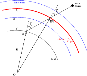
Figure 1: Schematic representation of an astronomical signal piercing the ionosphere. The solid blue curves delineate the ionosphere. The thick red curve is the ionospheric thin shell approximation, and the thin black curve delineates the surface of the Earth.

Given the triangle defined by the points A, O, and IPP (Fig. 1), the value of the zenith angle ($\zeta^{\prime}$) at the IPP is derived using the law of sines:

$$\mathrm{sin}(\zeta^{\prime})=\frac{R}{R+h}\mathrm{sin}(\zeta),$$ (5)

where $h$ is the altitude of the ionospheric thin shell, as specified in the ionospheric electron density files described in §2.3. In a similar fashion, the other geographic and topographic parameters at the IPP can be calculated. Spherical trigonometry is used to calculate the latitude, longitude, and azimuth ($\varphi^{\prime}$) of the IPP.

2.3 Ionospheric electron density

Measurements of the ionospheric free electron content come from several sources. For example, the Center for Orbit Determination in Europe (CODE) offers global ionosphere maps (GIMs) in IONosphere map EXchange format (IONEX), available via anonymous ftp. IONEX files from CODE are derived from $\sim$ 200 GPS sites of the International Global Navigation Satellite System Service (IGS) and other institutions. Figure 2 illustrates twelve maps obtained from the CODE IONEX file for April 11th, 2011.

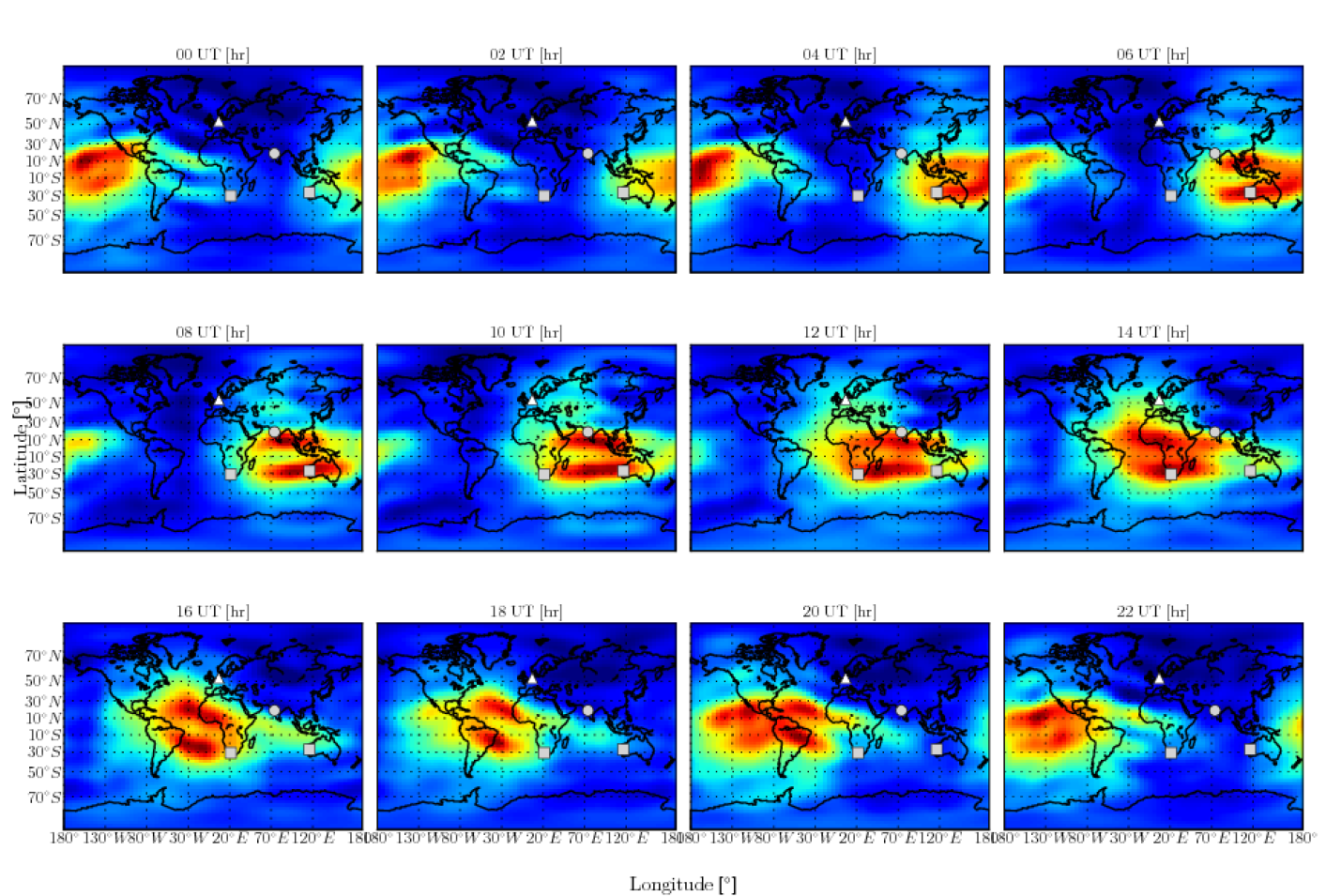
Figure 2: GIMs representing the VTEC across the globe for April 11th, 2011 (the date of the first LOFAR observing campaign, see §5) obtained courtesy of CODE. The maps range from minimum (blue) to maximum (red) VTEC values of $0.0-87.2$ TECU (1 TECU = 10¹⁶ electrons/m²). The triangles indicate the location of the LOFAR core stations in the Netherlands, the squares mark the SKA core sites in South Africa and Western Australia, and the circles indicate the site of the GMRT.

The IONEX files provide vertical total electron content (VTEC) values in a geographic grid ($\Delta_{\mathrm{lon.}}$ = 5^∘, $\Delta_{\mathrm{lat.}}$ = 2.5^∘). VTEC is defined as the integral of free electrons in the ionosphere along the zenith ($\zeta=0^{\circ}$) direction. The time resolution of the IONEX files provided by CODE is 2 hours. To increase the time resolution, ionFR creates new GIMs for every hour by using an interpolation scheme that takes the rotation of the Earth into consideration (Schaer et al., 1998, Eq. 3). The software interpolates the positional measurement grid to estimate the VTEC values at a given IPP for each hourly GIM. The interpolation uses a 4-point formula as in Fig. 1 of Schaer et al. (1998).

The final step in calculating the line-of-sight TEC is converting the VTEC to the slant TEC (TEC_LOS) as follows:

$$\mathrm{TEC}_{\rm LOS}=\frac{\mathrm{VTEC}}{\rm cos(\zeta^{\prime})}.$$ (6)

CODE also provides root-mean-square (RMS) VTEC maps that are geographically gridded in the same way as the VTEC maps. The uncertainties are calculated from these maps using Eq. 6. The 1-$\sigma$ uncertainties in the RMS VTEC maps are typically between 2 – 5 TECU.

ionFR will be regularly updated to allow a greater selection of TEC map sources. Maps with higher spatial and temporal resolution are desirable to trace ionospheric variations on shorter timescales and smaller spatial scales. For European telescopes, ionFR can also use TEC maps from the Royal Observatory of Belgium (ROB), which are derived from GPS data from a permanent European network. These TEC maps are more finely gridded than those from CODE ($\Delta_{\mathrm{lon.}}$ = 0.5^∘, $\Delta_{\mathrm{lat.}}$ = 0.5^∘) and have 15-minute time resolution (Fig. 3). They are also now publicly available via anonymous ftp, and are being produced since the beginning of 2012. Comparisons of ionFR-modeled Faraday depth based on the CODE/ROB maps are discussed in §5.1 (see Figs. 8 and 9).

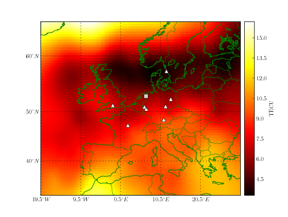
Figure 3: The VTEC across Europe for March 23rd, 2012 (the date of the third LOFAR campaign, see §5) at 00:00 UT, obtained courtesy of ROB. The square indicates the LOFAR core stations and the triangles represent the locations of the international stations.

2.4 The geomagnetic field

The Earth’s magnetic field is calculated using the eleventh generation of the International Geomagnetic Reference Field (IGRF11; Finlay et al., 2010) released in December 2009. The IGRF is derived by the International Association of Geomagnetism and Aeronomy (IAGA) every five years and is available to download. The IGRF11 is described as the negative gradient of a scalar potential, B= $-\nabla V$, which is a finite series of spherical harmonics. ionFR calls the IGRF11 to deliver the vector components of the geomagnetic field at the IPP. These point towards the north ($X$), east ($Y$), and radially towards the center of the Earth ($Z$). The $XYZ$ coordinates are local (orthogonal) coordinates, i.e. $X$ is not pointing in the direction of global north but to the local (tangential) north on the sky. The total magnetic field along the LOS at the IPP is then estimated as follows:

$$\mathrm{B}_{\rm LOS}=Z\mathrm{cos(\zeta^{\prime})}+Y\mathrm{sin(\zeta^{\prime})}\mathrm{sin(\varphi^{\prime})}+X\mathrm{sin(\zeta^{\prime})}\mathrm{cos(\varphi^{\prime})}.$$ (7)

2.5 Error propagation

The fractional uncertainties on $\mathrm{B}_{\rm LOS}$ compared with their central values ($\sigma_{\mathrm{B}_{\rm LOS}}/\mathrm{B}_{\rm LOS}$) are much smaller than the fractional uncertainties in the slant TEC ($\sigma_{\mathrm{TEC}_{\rm LOS}}/\mathrm{TEC}_{\rm LOS}$). Consequently, to determine the uncertainties on $\phi_{\mathrm{ion}}$, only the RMS slant TEC values are used. This results in uncertainties of 0.1 – 0.3 rad m^-2 in $\phi_{\mathrm{ion}}$ using the CODE global TEC maps. Assuming RMS values of 0.5 TECU for the ROB European TEC maps results in smaller uncertainties of 0.03 – 0.06 rad m^-2.

3 Ionospheric RM variation

Here we present some examples of ionFR-modeled ionospheric Faraday depths using TEC data from CODE. We illustrate both the $\phi_{\mathrm{ion}}$ variation within a day (for two epochs with differing levels of solar activity) as well as the longer-term variations with season and solar activity.

The modeled ionospheric Faraday rotations have been produced for the geographic coordinates of the LOFAR core and the LOS towards the supernova remnant Cassiopeia A (Cas A; RA = 23^h23^m27.9^s, DEC = +58^∘48^′42.4^′′). Cas A was selected because it is circumpolar as viewed from LOFAR (its minimum elevation is $\sim 22^{\circ}$). Therefore, ionFR can calculate the variation of $\phi_{\mathrm{ion}}$ for an entire day.

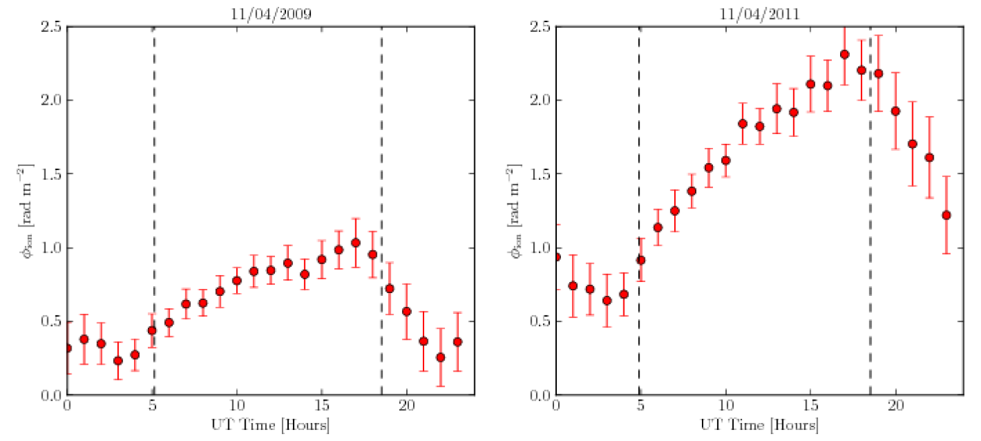
Figure 4: Prediction of the ionospheric Faraday rotation for two different epochs, as viewed from the LOFAR core along the LOS to Cas A. Left: Prediction when solar activity is near its minimum. Right: Prediction when the solar activity rises towards a new maximum, expected around May 2013. The dashed vertical lines mark the times of sunrise and sunset.

Figure 4 shows the variation in the modeled $\phi_{\mathrm{ion}}$ for two separate days: April 11th, 2009, close to the most recent minimum in solar activity, and April 11th, 2011, by which time solar activity had increase significantly. The next solar maximum is expected to be reached around mid 2013. These plots show the daily variation of $\phi_{\mathrm{ion}}$, increasing around sunrise and decreasing around sunset. This is expected due to the increase in the density of free electrons in the ionosphere from solar irradiation during the day. During night hours these free electrons begin to recombine with free ions. The degree of variation in $\phi_{\mathrm{ion}}$ is noticeably different on the two days. Near solar minimum (Fig. 4, left), the daily peak $\phi_{\mathrm{ion}}$ value is $\sim 1$ rad m^-2, while for the prediction two years later (Fig. 4, right), in which solar activity has increased, the level sometimes exceeds 2 rad m^-2. Note that these time-variable contributions are much larger than the formal uncertainties that are achievable through RM-synthesis techniques applied to low-frequency radio data (see §5).

Figure 5 (left) shows weekly averages of the daily maximum and minimum modeled $|\phi_{\mathrm{ion}}|$ since April 1998, along the LOS of Cas A as seen from the LOFAR core. According to the Space Weather Prediction Center (SWPC), Solar Cycle 23 started in May 1996 and ended in December 2008. ionFR was run for each day in Solar Cycles 23 and 24, until April 2012. The code produced daily files, each containing 24 values of $\phi_{\mathrm{ion}}$. From each file the daily maximum and minimum $|\phi_{\mathrm{ion}}|$ values were obtained. These values were averaged to give a representative maximum and minimum $|\phi_{\mathrm{ion}}|$ for every week since May 1996. Due to the incompleteness of GIMs within the IONEX files for the years 1996, 1997, and part of 1998, the ionospheric predictions are only shown since April 1998. The oscillation in the minimum $|\phi_{\mathrm{ion}}|$ is a well-known seasonal effect; more ionization is expected in summertime than in winter. In contrast, the maximum $|\phi_{\mathrm{ion}}|$ reveals that during the years of greatest solar activity (as reported by SWPC) several rad m^-2 can be reached, as viewed from the LOFAR core. It is also noted that when solar activity is at its highest, the maximum $|\phi_{\mathrm{ion}}|$ no longer appears to be dominated by seasonal variations.

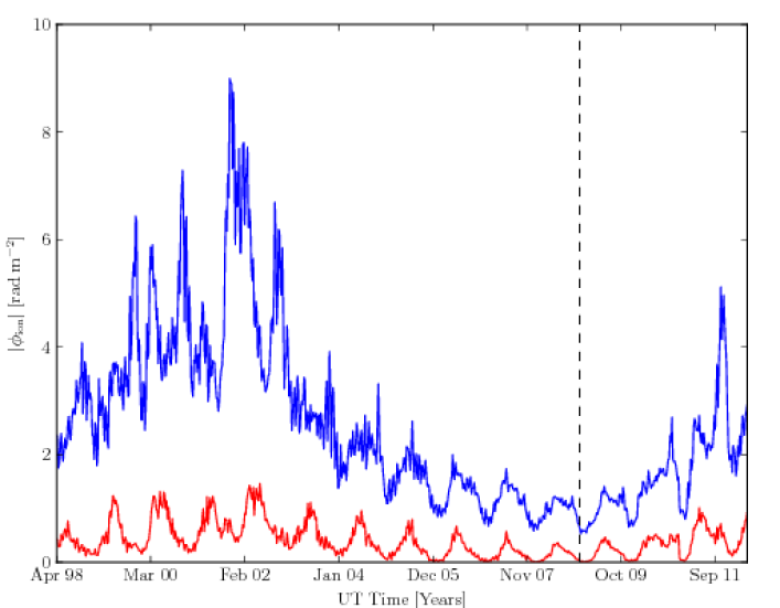
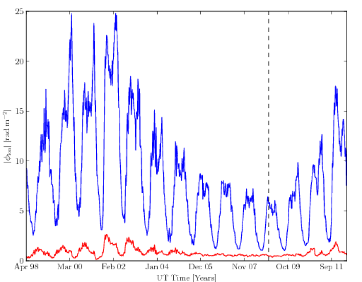
Figure 5: Weekly averages of the maximum and minimum (blue and red lines, respectively) absolute ionospheric Faraday depth $|\phi_{\mathrm{ion}}|$ from April 1998 – 2012, as modeled by ionFR. The absolute value is shown because the ionospheric Faraday depth is positive or negative if observing from the northern or southern hemisphere, respectively. The dashed vertical lines represent the end of Solar Cycle 23 (December 2008) and beginning of the current Solar Cycle 24. Left: towards CasA, as viewed from LOFAR. Right: towards Eta Carinae, as viewed from an average of the SKA core sites in Western Australia and South Africa.

It is evident from Fig. 2 that the ionosphere above the two sites chosen for the SKA are subject to the Equatorial Ionization Anomaly (EIA). These two regions of enhanced plasma density are located approximately 15 degrees north and south of the magnetic dip equator (McDonald et al., 2011) and are the result of the equatorial fountain effect (Appleton, 1946). We note that the SKA will suffer far higher levels of ionospheric Faraday rotation than at the LOFAR sites, as the southern component of the EIA can pass directly above both locations. Figure 5 (right) illustrates this by showing a representative history of $|\phi_{\mathrm{ion}}|$ for the two proposed SKA core sites. Predictions for the two sites were made towards the same astronomical object and then averaged. The LOS chosen to generate the two predictions was towards Eta Carinae (RA = 10^h45^m03.6^s, DEC = -59^∘41^′04.0^′′), which is circumpolar as viewed from both proposed sites. As expected, we observe that $|\phi_{\mathrm{ion}}|$ can be much higher than for LOFAR (Fig. 5, left). The seasonal effect is clearly visible in the maximum $|\phi_{\mathrm{ion}}|$ curve. Additionally, Figure 2 shows that during 12 hours the TEC and hence ionospheric RM were subject to large variations ($>80$ TECU). These facts underline the vital importance of ionospheric calibration for polarimetric studies with the SKA — particularly during the day, but even at night.

Also, as seen in Fig. 2, the EIA passes very close to the site of the GMRT, located near Pune, India. Hence, polarimetric observations with the GMRT can also benefit greatly from ionFR, especially for achieving the full potential of its available bands below 300MHz.

4 RM-synthesis

RM, which quantifies the amount of Faraday rotation along the LOS, has commonly been determined as the gradient of the polarization angle ($\chi$) as a function of wavelength squared ($\lambda^{\mathrm{2}}$); see, e.g., Cooper & Price (1962), Rand & Lyne (1994), and Van Eck et al. (2011). These previous RM measurements assumed therefore a linear relationship between $\chi$ and $\lambda^{\mathrm{2}}$. Brentjens & de Bruyn (2005) further developed an alternative method to measure Faraday rotation called RM-synthesis, which was first proposed by Burn (1966) and is now increasingly used for such measurements (Heald et al., 2009; Pizzo et al., 2011, e.g.,). The benefits of using RM-synthesis are numerous. For instance, it minimizes or eliminates any n$\pi$ ambiguity, as opposed to the ‘gradient’ method in which $\chi$ can rotate by 180^∘ an arbitrary number of n times between data points at each $\lambda^{\mathrm{2}}$. It also uses the polarization information across the entire observing bandwidth simultaneously such that it is not necessary to detect polarization angles at each $\lambda^{\mathrm{2}}$. Additionally, it does not assume that there is a single RM towards the LOS, i.e. that the linear relationship between $\chi$ and $\lambda^{\mathrm{2}}$ holds.

Following Brentjens & de Bruyn (2005) we define the observed complex polarization vector $P$ ($Q$ + $iU$) as:

$$P(\lambda^{\mathrm{2}})=\int^{\mathrm{\infty}}_{\mathrm{-\infty}}F(\phi)\exp\left[2\mathit{i}\phi\lambda^{\mathrm{2}}\right]\mathrm{d}\phi,$$ (8)

where $F(\phi)$ is the intrinsic complex polarized surface brightness per unit Faraday depth, known as the Faraday dispersion function (FDF, or Faraday spectrum; Burn, 1966). Hence, Eq. 8 can be inverted to obtain the FDF from the observed complex polarization vector:

$$F(\phi)=\int^{\mathrm{\infty}}_{\mathrm{-\infty}}P(\lambda^{\mathrm{2}})\exp\left[-2\mathit{i}\phi\lambda^{\mathrm{2}}\right]\mathrm{d}\lambda^{\mathrm{2}}.$$ (9)

Polarization observations have a limited range in $\lambda^{\mathrm{2}}$ and $\lambda^{\mathrm{2}}\leavevmode\nobreak\ \leq\leavevmode\nobreak\ 0$ is not possible. Therefore, Brentjens & de Bruyn (2005) introduce a window function that is non-zero for all observed $\lambda^{\mathrm{2}}$ and zero otherwise. In practice, the integral in Eq. 9 is performed as a discrete sum such that for each discrete channel $i$ at $\lambda^{\mathrm{2}}_{i}$:

$$F(\phi)\approx\left(\sum^{N}_{i=1}\omega_{i}\right)^{\mathrm{-1}}\sum^{N}_{i=1}\omega_{i}P(\lambda_{i}^{\mathrm{2}})\exp\left[-2\mathit{i}\phi(\lambda_{i}^{\mathrm{2}}-\lambda_{\mathrm{0}}^{\mathrm{2}})\right],$$ (10)

where $\omega_{i}$ is the weight of channel $i$ and $\lambda_{\mathrm{0}}$ is the weighted average of the observed $\lambda^{\mathrm{2}}$. Considering this inversion as the ‘coherent’ addition of the observed polarization vectors (a polarization vector per channel) for a range of Faraday depths, the vectors will constructively interfere within the bandwidth for the Faraday depth of the observed source and will result in a peak at this $\phi$ in the FDF. To illustrate this, example FDFs obtained from LOFAR High-Band Antenna (HBA) and Low-Band Antenna (LBA) observations (see §5) are displayed in Fig. 6. Equation 10 is used to determine the FDF for the observations described here. The relationship between the input observed complex polarization vector and the output FDF is given by the rotation measure spread function (RMSF):

$$R(\phi)\approx\left(\sum^{N}_{i=1}\omega_{i}\right)^{\mathrm{-1}}\sum^{N}_{i=1}\omega_{i}\exp\left[-2\mathit{i}\phi(\lambda_{i}^{\mathrm{2}}-\lambda_{\mathrm{0}}^{\mathrm{2}})\right].$$ (11)

RM-synthesis is analogous to performing aperture synthesis imaging with an interferometer in the sense that both methods make use of Fourier transforms using discrete sampling in $\lambda^{2}$ and spatial frequency coordinates ($u,v,w$), respectively (Heald et al., 2009, e.g.,). Hence, the RMSF in Faraday space $\phi$ is analogous to the dirty beam in angular coordinates on the sky ($l,m$) (Bell & Enßlin, 2012). As such, fewer gaps in the sampling of $\lambda^{2}$ reduce the side lobes in the RMSF and using larger bandwidths in $\lambda^{2}$ space increases the resolution in $\phi$ space. The resolution in Faraday space can be quantified by the FWHM of the RMSF function,

$$\mathrm{FWHM}\approx\frac{3.8}{\lambda^{\mathrm{2}}_{\mathrm{max}}-\lambda^{\mathrm{2}}_{\mathrm{min}}}\leavevmode\nobreak\ {\mathrm{rad\leavevmode\nobreak\ m^{\mathrm{-}2}}},$$ (12)

where $\lambda_{\mathrm{min}}$ and $\lambda_{\mathrm{max}}$ are the shortest and longest observed wavelengths and the constant 3.8 is from Schnitzeler et al. (2009). Moreover, the uncertainty associated with locating the peak Faraday depth in the FDF can be determined in the same way as the uncertainty associated with locating the peak flux in an aperture synthesis image (Fomalont, 1999, see):

$$\sigma_{\phi}=\frac{\mathrm{FWHM}}{2\times\mathrm{S/N}},$$ (13)

where FWHM is the FWHM of the RMSF defined in Eq. 12 and S/N is the total polarized signal-to-noise ratio. Equation 13 is used to determine the error in the Faraday depth measurements presented here.

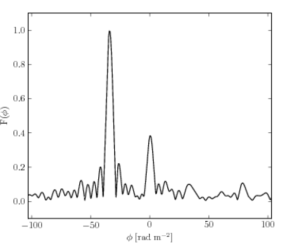
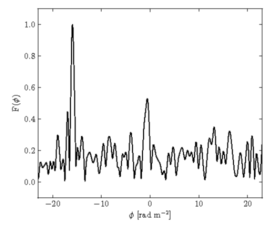
Figure 6: Examples of the absolute value of the normalized Faraday Dispersion Function (FDF), obtained from two LOFAR observations. The peaks at zero Faraday depth, $F(\phi\approx 0)$, indicate the instrumental response. Left: FDF obtained from a single 3-minute HBA observation ($119-125$ MHz) of PSR B2217+47. The peak at $F(\phi=-34.08\leavevmode\nobreak\ {\rm rad\leavevmode\nobreak\ m}^{-2})$ is the response due to the polarized flux of the pulsar. The FWHM of the RMSF is 6.6 rad m^-2. Right: FDF obtained from a single 3-minute LBA observation ($58-64$ MHz) of PSR B1919+21. The polarized flux of the pulsar is responsible for the peak at $F(\phi=-15.94\leavevmode\nobreak\ {\rm rad\leavevmode\nobreak\ m}^{-2})$. The FWHM of the RMSF is 0.84 rad m^-2.

5 Model comparison with observational data

5.1 LOFAR pulsar data

To measure Faraday depth variations in the ionosphere and to compare them with those modeled by ionFR, four bright polarized pulsars were observed using LOFAR (see Stappers et al., 2011, for a description of LOFAR’s pulsar observing modes). One or more pulsars were observed on four separate epochs, including times when the ionosphere was expected to be particularly dynamic (around sunrise and sunset). See Table 1 for a summary of these four observing campaigns.

The first campaign used the coherently combined LOFAR ‘Superterp’ to observe PSR B0834+06 in $7\times 10$-min integrations spaced every 50 min. These started 1.8 hr before sunset (18:25 UT) and continued until more than 2 hr after astronomical twilight (20:40 UT).

The second Superterp campaign observed PSR B0834+06 in $20\times 3$-min integrations spaced every 7 min. These started after astronomical twilight (04:11 UT) and continued until 1.5 hours after sunrise (06:08 UT).

The third Superterp campaign observed PSRs B1642$-$03, B1919+21 and B2217+47 by cycling consecutively through the three pulsars so that each was observed for $12\times 3$-min integrations spaced every 20 min. This enabled quasi-simultaneous measurements of the ionospheric Faraday depth variations towards three widely separated LOSs. These observations started before nautical twilight (04:16 UT) and ended two hours after sunrise (05:29 UT).

The fourth campaign observed PSR B0834+06 using the LOFAR Superterp stations and two international stations located near Nançay, France and near Onsala, Sweden. The pulsar was quasi-simultaneously observed by each station in $11\times 3$-min integrations spaced by 17 min. These were done during midday when the absolute TEC was expected to be relatively high. This enabled measurements of Faraday depth variations from three locations separated by long geographical baselines – 594 km minimum and 1294 km maximum distance, respectively.

No.	PSR	Date	Obs. duration	Sun[rise,set] time	LOFAR stations	Time obs.	No. obs.	Freq	Elevation	LOFAR obs. IDs
	(B-name)	(dd.mm.yyyy)	(hh:mm UT)	(hh:mm UT)		(min)		(MHz)	(deg)
1	B0834+06	11.04.2011	16:40 – 22:50	18:25	CS00[2-7]HBA	10	7	120–126	20 – 45	L25152 – L25158
2	B0834+06	20.10.2011	04:20 – 07:33	06:08	CS00[2-7]HBA	3	20	129–140	37 – 44	L32350 – L32369
3	B1642$-$03	23.03.2012	04:08 – 07:40	05:29	CS00[2-7]HBA	3	12	119–125	16 – 34	L53966 – L53977
3	B1919+21	23.03.2012	04:04 – 07:36	05:29	CS00[2-7]LBA	3	12	58–64	45 – 59	L53942 – L53953
3	B2217+47	23.03.2012	04:12 – 07:44	05:29	CS00[2-7]HBA	3	12	119–125	37 – 72	L53990 – L54001
4	B0834+06	10.07.2012	11:20 – 14:43	N/A	CS00[2,3,5-7]HBA	3	11	119–129	38 – 44	L61473 – L61483
4	B0834+06	10.07.2012	11:25 – 14:48	N/A	FR606HBA	3	11	119–129	42 – 49	L61532 – L61542
4	B0834+06	10.07.2012	11:30 – 14:53	N/A	SE607HBA	3	11	119–129	32 – 39	L61520 – L61530

Table 1: Summary of the four LOFAR pulsar observing campaigns. Columns 1–11 show the number of the observing campaign, pulsar B names, date, duration, time of sunset or sunrise during the observations, LOFAR station(s) (CS00[2-7] indicate the LOFAR ‘Superterp’ stations combined in tied-array mode, HBA and LBA indicate High-Band Antenna stations and Low-Band Antenna stations, respectively), individual observation integration times, total number of observations, frequency range, elevation range, and LOFAR observation identification numbers (obs. IDs).

In all cases, data were written as complex values for the two orthogonal linear polarizations. The data were recorded using the 200 MHz clock mode, which provides multiple 195.3125 kHz subbands that are further channelized by an online poly-phase filter to 12.2 kHz channels with a time resolution of 81.92 $\upmu$s. Due to limitations on the data rate at the time of observation, $6-11$ MHz of bandwidth were recorded. In comparison, 80 MHz of bandwidth can now be recorded by LOFAR in this mode. Nonetheless, given the low central observing frequencies ($\sim 125$ MHz) the recorded bandwidths were still more than adequate to achieve precise RM measurements. The complex values were converted to 8-bit samples offline and then coherently dedispersed and folded using the dspsr program (van Straten & Bailes, 2011). Radio frequency interference (RFI) was removed using the pazi program of PSRCHIVE (Hotan et al., 2004).

The reduced data were analyzed using an RM-synthesis program in order to determine a precise Faraday depth for each individual observation. For each data set, the Stokes parameters ($IQUV$) and associated uncertainties for each frequency channel were output for the pulsed section of the pulsar profile using the PSRCHIVE program rmfit. The frequency, $Q$ and $U$ information were used as the input to the RM-synthesis program, which calculated the FDF as a discrete sum for Faraday depths $-$50 $\leq$ $\phi$ $\leq$ 50 rad m^-2 in steps of 0.001 rad m^-2 using Eq. 10 (see Fig. 6 for two examples of these). The peak associated with the instrumental DC signal at $\sim$0 rad m^-2 Faraday depth (Geil et al., 2011, see, e.g.,) was subtracted from the FDF before determining the peak associated with the Faraday depth towards each pulsar LOS. This had no effect on the Faraday peaks of the pulsars since the known RM values (ATNF pulsar catalog; Manchester et al., 2005) are $>$ $2\times$FWHM of the RMSF, see Eq. 12. The Faraday depth at which the peak in the FDF occurred was assumed to be the measured Faraday depth of the ISM and ionosphere towards the pulsar, $\phi_{\mathrm{ISM}}+\phi_{\mathrm{ion}}$. For each observing campaign, we estimated the instrumental error by measuring the Faraday depth of the instrumental polarization peak around 0 rad m^-2 in the FDF of each observation, weighted by the S/N, and taking the 0 rad m^-2 $\pm$1$\sigma$ limits (Table 2). This demonstrated that larger bandwidth observations with higher S/Ns also tended to reduce the scatter in instrumental Faraday depth around 0 rad m^-2. The total error on the Faraday depth was taken to be the formal error from Eq. 13 added in quadrature with the instrumental error. The linear polarization had S/N $>30$ for all observations; this is well above the threshold necessary for reliable Faraday depth measurements (see Macquart et al., 2012, and references therein). While we have shown that LOFAR provides reliable Faraday depths, we note that absolute polarization calibration (e.g. to determine absolute polarization angles) has not yet been applied to the data.

The observed and ionFR-modeled Faraday depths as a function of time for the four LOFAR observing campaigns are plotted in Figs. 7, 8 and 9. In general, the modeled and observed Faraday depth variations agree very well. However, there are a few instances where the observed and modeled values differ by more than 1$\sigma$. The measured RMs could still be affected by interference in some cases and it is also quite possible that there are unmodeled ionospheric variations on short timescales (see also §6). TEC data from CODE was used for the B0834+06 sunset and sunrise campaigns. CODE and ROB TEC data were both available for the observations which took place in 2012 and are compared in Figs. 8 and 9. In each case, there is a clear trend in the Faraday depth as a function of time. At sunrise and sunset there is a particularly distinct variation in Faraday depth of approximately 2 rad m^-2, as expected (cf. Fig. 4). Even during midday, Fig. 9, when the absolute TEC is expected to be high but relatively constant (e.g., Kassim et al., 2007, Fig. 14), smaller variations in Faraday depth are still evident and well modeled in general.

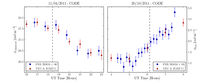
Figure 7: Observed Faraday depths, $\phi_{\mathrm{observed}}$, and ionFR-modeled ionospheric Faraday depths, $\phi_{\mathrm{ion}}$, towards PSR B0834+06 as a function of time (observations: blue circles, left axis labels; model: red triangles, right axis labels). Only CODE TEC data was available for these predictions. Left panel: seven LOFAR Superterp HBA observations during sunset. Right panel: twenty LOFAR Superterp HBA observations during sunrise. The vertical dashed lines indicate the time of sunset and sunrise, respectively. The offsets between $\phi_{\mathrm{observed}}$ and $\phi_{\mathrm{ion}}$ for the sunset and sunrise campaigns are 25.15 $\pm$ 0.18 and 24.94 $\pm$ 0.24 rad m^-2, respectively.

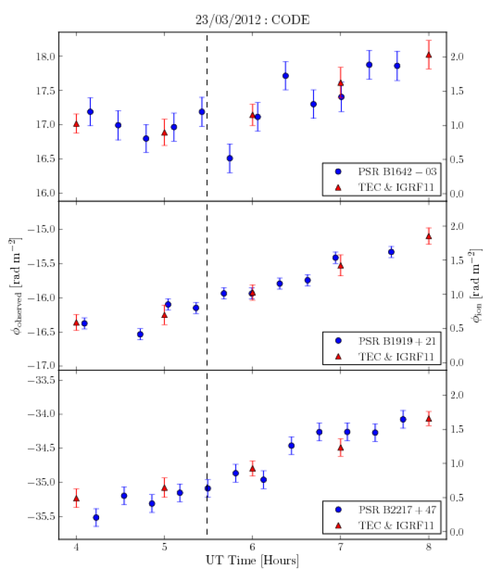
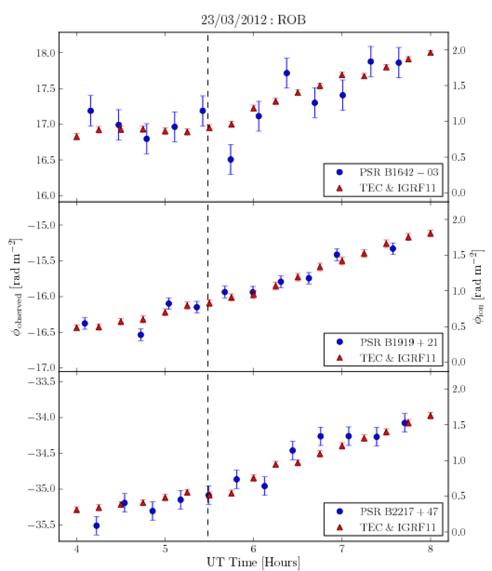
Figure 8: Observed Faraday depths, $\phi_{\mathrm{observed}}$, and ionFR-modeled ionospheric Faraday depths, $\phi_{\mathrm{ion}}$, towards three pulsars as a function of time during sunrise (observations: blue circles, left axis labels; model: red triangles, right axis labels). Upper panels: twelve LOFAR Superterp HBA observations of PSR B1642$-$03. Middle panels: twelve LOFAR Superterp LBA observations of PSR B1919+21. Lower panels: twelve LOFAR Superterp HBA observations of PSR B2217+47. The vertical dashed lines indicate the time of sunrise. $\mathrm{(a)}$ shows the ionFR model using CODE TEC data and IGRF11. $\mathrm{(b)}$ shows the ionFR model using ROB TEC data and IGRF11.

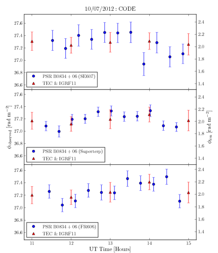
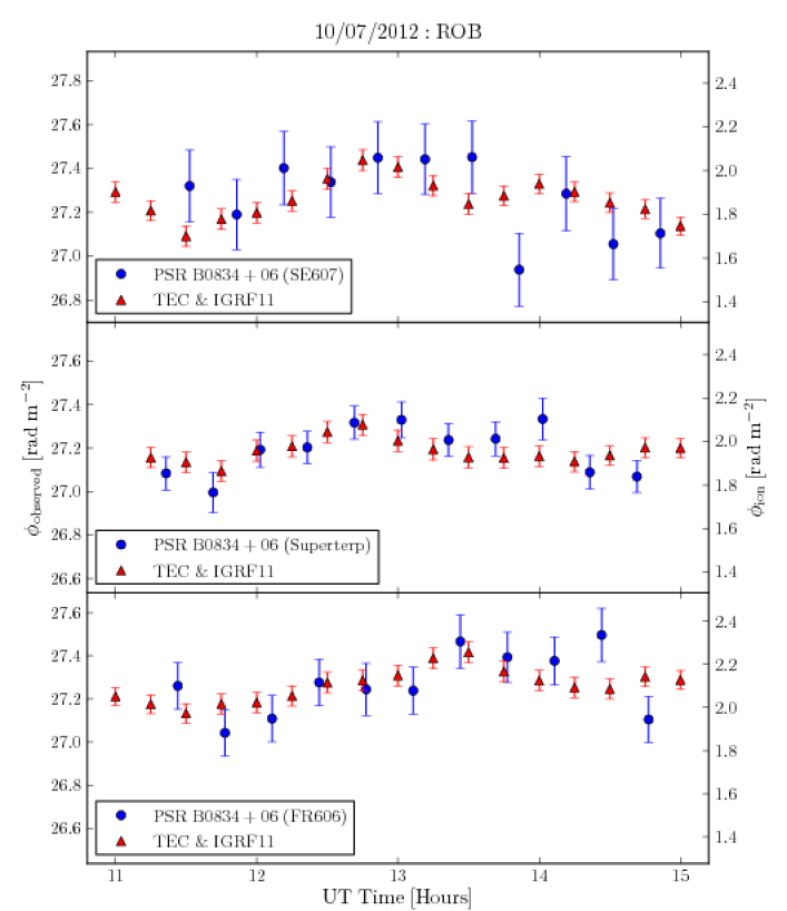
Figure 9: Observed Faraday depths, $\phi_{\mathrm{observed}}$, and ionFR-modeled ionospheric Faraday depths, $\phi_{\mathrm{ion}}$, towards B0834+06 as a function of time during midday (observations: blue circles, left axis labels; model: red triangles, right axis labels). Upper panels: eleven LOFAR HBA observations using the international station near Onsala, Sweden. Middle panels: eleven LOFAR Superterp HBA observations. Lower panels: eleven LOFAR HBA observations using the international station near Nançay, France. $\mathrm{(a)}$ shows the ionFR model using CODE TEC data and IGRF11. $\mathrm{(b)}$ shows the ionFR model using ROB TEC data and IGRF11.

Figs. 8 and 9 compare the modeled Faraday depths using CODE and ROB TEC data. In both cases, the observations and model show good agreement, although it is evident that there are variations on timescales less than one hour which are not resolved in the model using CODE data. The model using ROB TEC data more accurately fits the observations. The finer griding and smaller RMS available with the ROB TEC data also allows smaller fluctuations in Faraday depth to be resolved. For the observations of B0834+06 using the Superterp and international stations over midday, Fig. 9, this is especially significant, where the variations in the data appear on shorter timescales and in Faraday depths within the error bars of the model using CODE data. The model output of ionFR shows good agreement with the measured Faraday depths for all of the LOFAR observing campaigns depicted in Figs. 7, 8 and 9. Therefore, this model was used to subtract the contribution of the ionospheric Faraday depth from the measurements in order to determine the Faraday depth of the ISM, $\phi_{\mathrm{ISM}}$, in the direction of these pulsars.

To determine $\phi_{\mathrm{ISM}}$ for each pulsar, the constant offset which yielded the minimum weighted chi-squared value between the pulsar Faraday depth measurements and the ionospheric modeled Faraday depths from ionFR was used (see Table 2). Using the CODE data, the reduced chi-squared values range from 0.4 – 1.0, whereas with the ROB data the reduced chi-squared values range from 0.9 – 1.3. The residual differences between the observations and model may be due to small scale variations in the ionosphere which affect the observations but which are not resolved due to the time resolution of the TEC data. The standard deviations of $\phi_{\mathrm{observed}}-\phi_{\mathrm{ion}}$ divided by the square root of the number of measurements in each observational campaign range from 0.03 – 0.09 rad m^-2 for the CODE output and from 0.02 – 0.07 rad m^-2 for the ROB output. This indicates that both fit the measurements well, although the ROB data gives reduced chi-squared values closer to 1 and smaller errors due to the smaller uncertainties compared with the CODE maps. Also, both sources of TEC maps give consistent results, where all $\phi_{\mathrm{ISM}}$ values obtained using CODE and ROB data agree within 1-$\sigma$ for the same observing campaign and LOS. The Faraday depth values for B0834+06 obtained from the three observational campaigns over six months apart also agree at or below the 2-$\sigma$ level for both CODE and ROB data. The weighted mean for all CODE and ROB data available for B0834+06 gives $\phi_{\mathrm{ISM}}=25.12\pm 0.07$ rad m^-2 (5 LOSs) and $\phi_{\mathrm{ISM}}=25.26\pm 0.05$ rad m^-2 (3 LOSs), respectively. Although there are two more data sets with CODE data available, the errors assumed for the ROB data are smaller. It is worth noting that these are among the most precise pulsar-derived $\phi_{\mathrm{ISM}}$ measurements ever obtained (Manchester et al., 2005, see ATNF catalog), and improve significantly on the precision of previous RM measurements for these pulsars.

In order to determine the Faraday depth of B0834+06 using an independent instrument, on April 22nd, 2012 at 16:50 UT we performed a 20-minute observation of PSR B0834+06 using the WSRT with the PuMaII pulsar backend (Karuppusamy et al., 2008) from 310 to 390 MHz. We recorded baseband data, which were folded, dedispersed and subsequently analyzed using the same RM-synthesis method described above, yielding $\phi_{\rm observed}=28.2\pm 1.8$ rad m^-2. The ionFR code predicts $\phi_{\mathrm{ion}}=2.75\pm 0.15$ rad m^-2, using CODE maps, for the given time and LOS of this observation, resulting in a corrected value of $\phi_{\mathrm{ISM}}^{WSRT}=25.4\pm 1.8$ rad m^-2. Using ROB maps we calculated a corrected value of $\phi_{\mathrm{ISM}}^{WSRT}=25.1\pm 1.5$ rad m^-2. These values are in excellent agreement with the more precise value derived from the LOFAR observations. The precision of the WSRT measurement is lower in part because of the higher observing frequency, see Eqs. 12 and 13. This demonstrates the power of low-frequency observations for the purpose of determining accurate $\phi_{\mathrm{ISM}}$.

Our measured Faraday depths are consistent with previously published measurements for these pulsars, but are significantly more precise. The values of $\phi_{\mathrm{ISM}}$ obtained from the LOFAR observations of B0834+06 agree to within 2.5 $\sigma$ of the catalog value for this pulsar, RM_psrcat = 23.6 $\pm$ 0.7 rad m^-2. It is unclear, but likely, that the catalog value was calibrated for ionospheric Faraday rotation (see Hamilton & Lyne, 1987, §2). That paper also states that the ionosphere contributes 1$-$8 rad m^-2 to other observations, using either a geostationary satellite or an ionosonde, and that the subtraction of this introduces uncertainties of approximately 1$-$2 rad m^-2. The 2.5-$\sigma$ difference between the $\phi_{\mathrm{ISM}}$ obtained using LOFAR and the ATNF catalog value determined in 1987, plus the possibility that pulsar RMs may change on multi-year timescales (Weisberg et al., 2004, e.g.,) due to variations in the polarized pulsar emission and/or electron density changes along the LOS through the ISM, provided the motivation for the recent independent comparison observation of PSR B0834+06 using the WSRT.

The values of $\phi_{\mathrm{ISM}}$ obtained for the three pulsars observed quasi-simultaneously are also very precise and are in excellent agreement with those of the ATNF pulsar catalog. Prior measurements for B1642$-$03 and B1919+21, also calibrated for ionospheric Faraday rotation using geostationary satellite and ionosonde data, give RM${}_{\mathrm{ISM}}=15.8\pm 0.3$ rad m^-2 and RM${}_{\mathrm{ISM}}=-16.5\pm 0.5$ rad m^-2, respectively (Hamilton & Lyne, 1987), and are also in good agreement within 1 $\sigma$ of the values obtained in this work (ROB-subtracted values $\phi_{\mathrm{ISM}}=16.04\pm 0.18$ rad m^-2 and $\phi_{\mathrm{ISM}}=-16.92\pm 0.07$ rad m^-2). A prior measurement for B2217+47, RM${}_{\mathrm{ISM}}=-35.3\pm 1.8$ rad m^-2, also calibrated for ionospheric Faraday rotation using a geostationary satellite (Manchester, 1972), is also in good agreement within 1 $\sigma$ of the value derived here (ROB-subtracted value $\phi_{\mathrm{ISM}}=-35.60\pm 0.11$ rad m^-2).

Together these observations provide a convincing verification of the accuracy of the ionFR model and demonstrate the ability to derive Faraday depths resulting solely from the ISM by robustly removing the time and direction-dependent Faraday depth introduced by the ionosphere, even during some of the most turbulent periods expected in daily ionospheric variations; see §6 for further discussion.

PSR	Date	Telescope	Station(s)	FWHMRMSF	$\sigma_{\mathrm{inst}}$	$\phi_{\mathrm{ISM}}^{\mathrm{CODE}}$	$\chi^{2}_{\mathrm{red}}$	$\phi_{\mathrm{ISM}}^{\mathrm{ROB}}$	$\chi^{2}_{\rm red}$	RM${}_{\mathrm{ISM}}^{\mathrm{psrcat}}$
	[dd.mm.yy]			[rad m-2]	[rad m-2]	[rad m-2]	CODE	[rad m-2]	ROB	[rad m-2]
B0834+06	11.04.11	LOFAR	Superterp	6.2	0.20	25.15 $\pm$0.18	0.52	N/A	N/A	23.6 $\pm$ 0.7
B0834+06	20.10.11	LOFAR	Superterp	9.4	0.20	24.94 $\pm$ 0.24	0.64	N/A	N/A	23.6 $\pm$ 0.7
B1642$-$03	23.03.12	LOFAR	Superterp	6.6	0.20	15.98 $\pm$ 0.23	0.8	16.04 $\pm$ 0.18	1.3	15.8 $\pm$ 0.3
B1919+21	23.03.12	LOFAR	Superterp	0.8	0.08	-16.95 $\pm$ 0.12	0.5	-16.92 $\pm$ 0.07	1.3	-16.5 $\pm$ 0.5
B2217+47	23.03.12	LOFAR	Superterp	6.6	0.13	-35.72 $\pm$ 0.15	1.0	-35.60 $\pm$ 0.11	1.1	-35.3 $\pm$ 1.8
B0834+06	22.04.12	WSRT	N/A	12.0	1.2	25.4 $\pm$ 1.8	N/A	25.1 $\pm$ 1.5	N/A	23.6 $\pm$ 0.7
B0834+06	10.07.12	LOFAR	Superterp	4.2	0.07	25.16 $\pm$ 0.13	0.5	25.23 $\pm$ 0.08	0.9	23.6 $\pm$ 0.7
B0834+06	10.07.12	LOFAR	FR606	4.2	0.10	25.21 $\pm$ 0.15	0.4	25.16 $\pm$ 0.10	1.2	23.6 $\pm$ 0.7
B0834+06	10.07.12	LOFAR	SE607	4.2	0.15	25.22 $\pm$ 0.18	0.6	25.39 $\pm$ 0.14	1.0	23.6 $\pm$ 0.7

Table 2: Summary of results from the four LOFAR pulsar observing campaigns and WSRT observation. Columns 1–11 show the pulsar observed, date (see Table 1 for specific times), the telescope, the LOFAR stations (if applicable, see Table 1 for specific station names), the FWHM of the RMSF from RM-synthesis, the error introduced by instrumental effects $\sigma_{\mathrm{inst}}$, the Faraday depth of the ISM towards the pulsar $\phi_{\mathrm{ISM}}$ as determined using the CODE TEC maps, the reduced chi-squared value $\chi^{2}_{\mathrm{red}}$ for comparison between the ionospheric Faraday depths from ionFR using CODE TEC data and the observed Faraday depths, the Faraday depth of the ISM towards the pulsar $\phi_{\mathrm{ISM}}$ as determined using the ROB TEC maps, the reduced chi-squared value for comparison between the ionospheric Faraday depth produced from ionFR using CODE TEC data and the observed Faraday depths. The final column gives the catalog RM value from psrcat (Manchester et al., 2005) for comparison. Note that ROB TEC maps were not available for the observations of B0834+06 taken in 2011. Since a single observation was obtained with WSRT, the reduced chi-squared value is not applicable because the Faraday depth of the ISM was determined by subtracting the Faraday depth of the ionosphere from the observed Faraday depth.

5.2 WSRT imaging data

Here we compare the ionFR-modeled Faraday depths with archival 118.2-MHz WSRT observations of PSR B1937+21.

PSR B1937+21 was observed with the WSRT Low Frequency Front Ends on 25 March 2005 for 3 hours following sunrise to monitor ionospheric Faraday rotation. The observed polarization angle at 118.2 MHz is shown in Fig. 10 and it is seen to increase rapidly and smoothly. The polarization angle presented refers only to a 4 MHz band, from 116.05 – 120.34 MHz. The calibrated data were split into 30 time slots, of 6 minutes each, in order to produce a pair of Stokes $Q$ and $U$ maps for each slot. From the polarization maps we then calculated the polarization angle of PSR B1937+21.

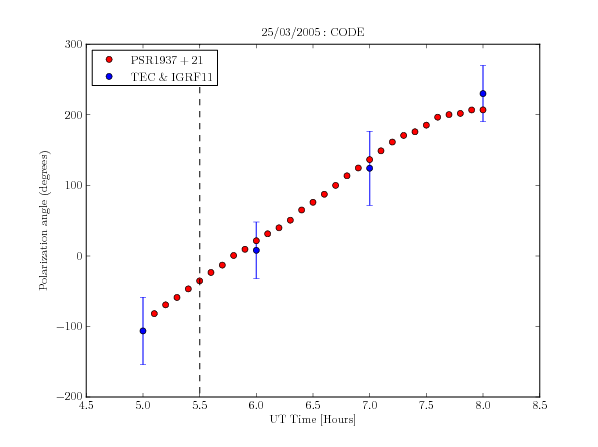
Figure 10: PSR B1937+21’s observed polarization angle compared with the predicted amount of rotation due to the ionosphere (red and blue points, respectively). The errors on the polarization angles for the WSRT data are less than 2 degrees and are not visible in the plot. The vertical dashed line marks the time of sunrise.

Fig. 10 also shows the predicted rotation due to the ionosphere. This was calculated by modeling the $\phi_{\mathrm{ion}}$ using CODE TEC data (no ROB data is available prior to 2012), and then converting the ionospheric Faraday depths into polarization angles at 118.2 MHz. After removing a constant offset, the modeled Faraday depths and observation match very well. This comparison provides further verification of ionFR-modeled Faraday depths and also shows that the ionospheric correction can be done for interferometric imaging data.

As this example shows, low-frequency observations lasting a few tens of minutes or more suffer depolarization from variable ionospheric Faraday rotation; in this case, the polarization angle has made almost a full turn within 3hrs. The time-variable ionospheric Faraday depth will lead to misalignment between the polarization vectors, which therefore results in significant signal loss. Even an instantaneous measurement gives a Faraday depth that is systematically biased by $\pm 0.25-2.5$ rad m^-2 or more, which can be a large fraction of the total measured Faraday depth for nearby sources ($d<2$ kpc), greatly impeding our ability to use these as probes of the local interstellar magnetic field.

6 Discussion

The Faraday depths of the ISM towards PSRs B0834+06, B1642$-$03, B1919+21 and B2217+47 presented here (Table 2) are some of the first determined using the RM-synthesis technique and are among the most precise Faraday depth measurements ever made towards a pulsar. In the ATNF catalog, there are only a dozen measurements with absolute precision $\leq 0.2$ rad m^-2, determined for some of the brightest known pulsars. The fact that the Faraday depths obtained here are also in excellent agreement with the catalog and/or alternatively determined values also demonstrates the robustness of ionFR for subtracting the $\phi_{\mathrm{ion}}$ contribution and hence for allowing us to reap the benefits of low-frequency measurements.

Using multi-beaming capabilities (Stappers et al., 2011), LOFAR will provide high-precision Faraday depth measurements for hundreds of nearby pulsars, which can be used to probe the interstellar magnetic field of the Galaxy (e.g. Sobey et al. 2013, in preparation). Since the observations presented here used just a tenth of the now-available LOFAR bandwidth, the prospects for even higher-precision Faraday depth measurements are excellent, especially using LOFAR LBA observations ($10-90$ MHz). However, with the TEC data available from ROB these will be limited to precisions of approximately 0.05 rad m^-2 because of the systematic uncertainty provided by the RMS VTEC maps. In other words, more sophisticated calibration techniques will need to be devised in order to reap the full benefit of LOFAR’s low observing frequencies and large fractional bandwidth. For instance, it is possible to measure time-dependent, differential TEC and Faraday rotation between LOFAR stations using visibility data from observations of bright (even unpolarised) calibrators. These data can be combined with magnetic field models in order to predict the absolute Faraday depth, in addition to using the TEC data described here for comparison. This is currently being investigated using LOFAR long-baseline observations, but will be less suitable for more compact array designs (e.g., LOFAR pulsar observations typically use only the 2-km core of the array). Higher-precision Faraday depth measurements are especially important for determining possible long-term variations of the Faraday depth of pulsars due to fluctuations in their magnetosphere or the ISM (Weisberg et al., 2004, e.g.,), particularly as some pulsars have large relative velocities.

Calibrating for $\phi_{\mathrm{ion}}$ is also important for higher-frequency observations. Assuming a bandwidth of 1.21 – 1.51 GHz, such as that of the multibeam receiver used at the 100-m Effelsberg radio telescope (Barr et al., 2013) , the theoretical FWHM of the RMSF is 173 rad m^-2. This yields an uncertainty in Faraday depth of 8.7 rad m^-2 given a S/N of 10, which is comparable to the $\phi_{\mathrm{ion}}$ reached during solar maximum as Fig. 5 (left) shows. Given larger bandwidths, such as those planned for the SKA and its pathfinders, this problem becomes worse and is relevant even during night-time and solar minimum. It is also clear that corrections for the ionospheric Faraday depth are important for observations of pulsars and extragalactic sources, particularly towards the halo of the Galaxy, since the Faraday rotation expected is often much lower than those located towards the plane. For the 650 pulsars with rotation measure data, 284 of these are located over 300 pc above or below the galactic plane and have a median rotation measure of $\sim$39 rad m^-2. Ionospheric Faraday depth can thus contribute significantly to the total observed Faraday depth, especially at times near solar maximum or when observing from lower latitude sites.

The TEC maps from ROB will help to perform differential Faraday rotation studies between LOFAR core stations and the international stations. Fig. 3 shows a VTEC map from ROB over Europe. It is clear that the international stations are subject to different ionospheric conditions than the core, which results in different amounts of Faraday rotation for the signals arriving at each station. This effect needs to be calibrated for before combining all the LOFAR stations to carry out polarization studies. On the other hand, to better understand the ionospheric variations above just the Dutch LOFAR stations (max. baseline $\lesssim$ 100 km), better geographically resolved TEC maps are needed. Alternatively, raw, dual-frequency GPS data should be directly analyzed. Raw GPS data is also desirable to use when short timescale ionospheric changes (on the order of seconds to a few minutes) need to be studied. For arrays located in Europe this is possible due to the considerable number of GPS stations from the permanent European network. However, this is not yet the case for arrays like the GMRT or future SKA. For instance, in India there is only one active station (near Bangalore) which is part of the IGS network. This is also the case for South Africa and Western Australia, where there are a few more stations but they are very far apart. Regional dedicated networks, like in Europe, are needed for these arrays in order to gain a more detailed picture of the ionospheric sky over these sites. Alternatively, high accurate ionospheric corrections for the SKA could be possible through its own imaging data; a route being explored, as previously mentioned, for LOFAR.

A single LBA station operating at 20 MHz has a beam width of $\sim$ 13^∘, which spans less than 2 cell widths in the ROB TEC maps. This is because each of the cells (0.5^∘) extends $\sim$ 60 km at the altitude of the ionospheric thin shell, which corresponds to a resolution of $\sim$ 7.5^∘ in the plane of the sky. When using ROB data, this implies that we expect to predict the same ionospheric Faraday rotation for any source located within a radius of 7.5^∘.

We are expanding ionFR to support also the use of TEC data from the last release of the IRI (IRI-2007 ). This addition will allow access to TEC data from before 1995. This type of data was not included in the analysis herein due to the fact that no uncertainties are available for the IRI.

To further improve the accuracy of the ionFR-modeled Faraday depths, the Earth will be considered as an ellipsoid and also the various ionospheric layers (D, E, and F) can be treated. A three-dimensional model for the ionosphere should also be possible using ray tracing for three-dimensional tomography of the ionosphere (Bust & Mitchell, 2008, e.g.,). An indication that this may be needed for future high-accuracy Faraday depth determinations with LOFAR is the increase in the derived Faraday depth of the ISM towards B0834+06 as a function of latitude in the international station observations, see Fig. 11. Since the elevation of the pulsar is lower at higher geographic latitudes in these quasi-simultaneous observations, the LOS towards B0834+06 passes through a larger ionospheric depth as seen from Sweden compared with the Netherlands and France. Fig. 11 shows how the $\phi_{\mathrm{ISM}}$ determined at three latitudes appears to follow a similar trend to the airmass. Therefore, a correction similar to, although not quite as large as, the airmass may be needed (Wielebinski & Shakeshaft, 1962, e.g.,).

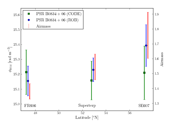
Figure 11: The measured Faraday depth of the ISM, $\phi_{\mathrm{ISM}}$, towards PSR B0834+06, as determined from HBA observations using the LOFAR FR606, Superterp and SE607 stations. These are plotted as a function of the geographic latitudes of the stations. The data points are offset slightly in latitude for ease of comparison. The measurements are also compared with the range in airmass calculated for the station location towards PSR B0834+06 for the duration of the observations (red triangles, right axis). The ionFR model was run using both TEC data from CODE (green squares) and ROB (blue points).

7 Conclusions

We have presented ionFR, a code that models the ionospheric Faraday rotation using publicly available TEC maps and the IGRF11. In §3 we show modeled ionospheric Faraday depths for changing levels of solar activity and different geographic locations. In §5 we compare ionFR-modeled Faraday depths with low-frequency data from LOFAR and the WSRT. These observational comparisons demonstrate the robustness and accuracy of the modeled data.

We have shown in §5.1 that calibrating LOFAR data with ionFR provides very high-precision pulsar RMs (absolute error $\lesssim 0.1$ rad m^-2). The applicability of precise RMs is broad. For instance, precise RMs can be used to map the structure of the Galactic magnetic field. Also, it is now possible to monitor pulsar RMs on multi-year timescales. For example, B0834+06, shows an apparent increase in its RM after $\sim$ 25 years, assuming previous ionospheric calibration was correct.

Our code represents an alternative, and moreover, a cheaper solution when no GPS receivers are co-located with the radio telescope carrying out the observation. Additionally, GPS receivers may need periodic maintenance, which requires an investment of time and money. Therefore, this code is put forward as a simple and costless method to the community to predict and correct for ionospheric Faraday rotation.

ionFR will be used to correct for the ionospheric Faraday rotation in projects such as the WSRT Continuum Legacy Survey at 350 MHz: Low-frequency Galaxy Continuum Survey (targets were observed in 2012), the LOFAR Magnetism Key Science Project (Anderson et al., 2012, MKSP;) and the Polarisation Sky Survey of the Universe’s Magnetism (Gaensler et al., 2010, POSSUM;) project planned with the Australian Kilometre Array Pathfinder (Johnston et al., 2007, ASKAP;) telescope.

Lastly, Phase I of the SKA will provide an unprecedented low-frequency radio telescope, capable of making, e.g., a detailed map of the Galactic magnetic field structure through Faraday depth measurements of pulsars. However, given that the ionospheric equatorial anomaly sometimes passes directly over the two sites in South Africa and Western Australia, it will be crucial to have a robust and accurate calibration procedure in place to take full advantage of what the SKA has to offer.