Entanglement detection from conductance measurements in carbon nanotube Cooper pair splitters

Abstract

Spin-orbit interaction provides a spin filtering effect in carbon nanotube based Cooper pair splitters that allows us to determine spin correlators directly from current measurements. The spin filtering axes are tunable by a global external magnetic field. By a bending of the nanotube the filtering axes on both sides of the Cooper pair splitter become sufficiently different that a test of entanglement of the injected Cooper pairs through a Bell-like inequality can be implemented. This implementation does not require noise measurements, supports imperfect splitting efficiency and disorder, and does not demand a full knowledge of the spin-orbit strength. Using a microscopic calculation we demonstrate that entanglement detection by violation of the Bell-like inequality is within the reach of current experimental setups.

The controlled generation and detection of entanglement is a necessary step toward the goal of using quantum states for applications. In a solid state nanostructure this control ideally allows us to manipulate and detect entanglement between selected pairs of electrons. A promising source of entangled electron pairs is the Cooper pair splitter (CPS). It consists of a superconductor that injects Cooper pairs through two quantum dots (QDs) into two outgoing normal leads, designed such that the Cooper pair electrons preferably split and leave the superconductor over different leads but preserve their spin entanglement recher:2001 ; cps . Very recently several CPS experiments have been performed hofstetter:2009 ; herrmann:2010 ; hofstetter:2011 ; das:2012 ; schindele:2012 and Cooper pair splitting efficiencies up to 90% have been reached schindele:2012 . So far, however, a proof that the electrons remain entangled is still lacking.

The present experiments do not allow to resolve individual splitting events, and the results of the measurements are time averaged quantities, such as current or noise. These provide information on the average spin correlations of the injected Cooper pairs. In this Letter we demonstrate that this information can be extracted from the currents alone in a carbon nanotube (CNT) based CPS, if spin-orbit interaction (SOI) effects are taken into account cottet:2012 . This allows us to propose a general entanglement test, based on the Bell inequality clauser:1969 ; bell_solid_state , which does not require noise measurements note .

Indeed, the SOI in CNTs leads to unique spin-energy filtering properties that directly modulate the Cooper pair splitting current flowing out of the CPS, and ideally suppress any noise. From conductance measurements it is then already possible to reconstruct all spin correlators contained in the Bell inequality, thus avoiding the need of ferromagnetic contacts as spin filters, which are challenging to implement. Without noise measurements we also avoid the associated problem of electron fluctuations in the detectors hannes:2008 . The built-in energy filtering furthermore leads to an enhanced Cooper pair splitting efficiency veldhorst:2010 .

Figure 1: Double quantum dot CPS based on a bent CNT in an external magnetic field $\mathbf{B}$. Because of $\mathbf{B}$, SOI, and the bending angle $\theta_{CNT}$ of the CNT, the spin-valley degeneracy of the QD levels is lifted, and the resulting 4 levels (boxes) are spin polarized as indicated by the arrows (see also Fig. 2). The superconductor SC injects Cooper pairs (hourglass shape) that split onto the QDs and provide a current to the normal leads N that is modulated by the spin projections of the QDs (tunable by the gates $V_{L,R}$) and can be used to determine the spin correlators for the Bell inequality.

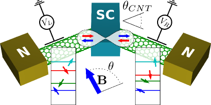
The proposed CPS setup is shown in Fig. 1 and consists of a regular double-QD CPS built from a single-wall CNT, yet made with a (naturally) bent CNT such that there is an angle $\theta_{CNT}$ between the QD axes. Alternatively, the QDs can be built from separate CNTs with similar diameters and an angle $\theta_{CNT}$ between them. The SOI spin splits the QD levels. In combination with a global magnetic field $\mathbf{B}$, the fourfold spin-valley degeneracy of the QD levels is completely lifted. The split levels provide a unique spin filter for electron transport with two spin projection axes per QD, filtering directly the injected Cooper pair current. Therefore, conductance measurements alone, at fixed $\mathbf{B}$, allow a reconstruction of all the spin correlators necessary for the Bell inequality. The spin projection axes are different in the two QDs due to the bending, and are tunable by $\mathbf{B}$. In the following we show that this tunability provides sufficient conditions for obtaining violations of the Bell inequality in an ideal CPS. We then proceed to a full microscopic calculation and demonstrate that the result remains robust under realistic conditions, as achievable by present experiments.

SOI in CNT quantum dots. CNTs are graphene sheets rolled into a cylinder. They preserve the graphene band structure with two Dirac valleys but have enhanced SOI contributions due to the curvature. The corresponding model, including the effect of $\mathbf{B}$, is described by the sum of the Hamiltonians izumida:2009 ; jeong:2009 ; klinovaja:2011a ; klinovaja:2011b

$$H_{0} =\hbar v_{F}\bigl{[}k_{t}^{0}\sigma_{1}+k\tau_{3}\sigma_{2}\bigr{]},$$ (1)

$$H_{cv} =\hbar v_{F}\bigl{[}\Delta k_{t}^{cv}\sigma_{1}+\Delta k_{z}^{cv}\tau_{3}\sigma_{2}\bigr{]},$$ (2)

$$H_{SOI} =\alpha\sigma_{1}S_{z}+\beta\tau_{3}S_{z},$$ (3)

$$H_{B} =\mu_{B}g\mathbf{B}\cdot\mathbf{S}/2+|e|v_{F}RB_{z}\sigma_{1}/2,$$ (4)

which are matrices in the space spanned by the graphene sublattice indices $\sigma=A,B$ (with Pauli matrices $\sigma_{1,2,3}$), the valleys $\tau=K,K^{\prime}=+,-$ (Pauli matrices $\tau_{1,2,3}$), and the spin projections $S=\uparrow,\downarrow$ (Pauli matrices $S_{x,y,z}$, with $S_{z}$ oriented along the CNT axis). $v_{F}$ is the Fermi velocity, $k_{t}^{0}$ the transverse quantized momentum (zero for metallic CNTs), $k$ the longitudinal momentum, $\Delta k_{t,z}^{cv}$ are momentum corrections induced by the curvature, $\alpha,\beta$ determine the SOI, $\mu_{B}$ is the Bohr magneton, $g=2$ the Landé $g$-factor, $e$ the electron charge, $R$ the CNT radius, and $B_{z}$ the component of $\mathbf{B}$ along $S_{z}$. We have neglected terms leading to the formation of Landau levels since at the considered sub-Tesla fields they are of no consequence. For a QD, $k$ is further quantized by the QD length bulaev:2008 ; weiss:2010 ; lim:2011 .

Because of its momentum independence, the SOI takes the role of an internal valley (and QD orbital) dependent Zeeman field $\tau\mathbf{B}_{SOI}$ along $S_{z}$, which combines with $\mathbf{B}$ to the effective field in each valley $\mathbf{B}^{\tau}_{\text{eff}}=\mathbf{B}+\tau\mathbf{B}_{SOI}$. These fields lift the spin degeneracy of the QD levels, while the orbital effect of Eq. (4) lifts the energy degeneracy between the two valleys for any $B_{z}\neq 0$. The QD levels turn into spin-valley-energy filters. The effective fields define the spin polarization axes $\mathbf{a}_{\tau}\propto\mathbf{B}_{\text{eff}}^{\tau}$, which are nonparallel if $\mathbf{B}^{K}_{\text{eff}}\neq\mathbf{B}^{K^{\prime}}_{\text{eff}}$, tunable by $\mathbf{B}$, and such that the spin-eigenstates in each valley $\left|\pm a_{\tau}\right\rangle$ fulfill $(\mathbf{S}\cdot\mathbf{a}_{\tau})\left|\pm a_{\tau}\right\rangle=\pm\left|\pm a_{\tau}\right\rangle$ (full polarization). If $P_{\pm a_{\tau}}=\left|\pm a_{\tau}\right\rangle\left\langle\pm a_{\tau}\right|$, spin measurements can be reconstructed by electron transport over the different QD levels by $(\mathbf{S}\cdot\mathbf{a}_{\tau})=P_{+a_{\tau}}-P_{-a_{\tau}}$.

Figure 2: Values $Q$ of the Bell equation (5) (left panel) for an ideal bent CNT-CPS as a function of in-plane $\mathbf{B}$-field rotation angle $\theta$, for the lowest valence band orbitals in a CNT of chirality (18,10), $|\mathbf{B}|=0.4$ T, $\theta_{CNT}=30^{\circ}$, $\alpha=-0.08$ meV, $\beta=-0.15$ meV, and QD lengths of 200 nm. For this situation, $|\mathbf{B}|/|\mathbf{B}_{SOI}|\approx\mu_{B}g|\mathbf{B}|/2|\alpha-\beta|=0.34$. The horizontal lines mark the threshold $Q=2$ and the maximal possible $Q=2\sqrt{2}$. The right panels show the $\theta$ dependence of the level energies of both QDs. The spectra are identical up to the shift by $\theta_{CNT}$ marked by the vertical dashed lines. The arrows indicate the spin polarizations in a global spin basis, as used for the determination of $Q$.

Bell test in an ideal CNT-CPS. In the double-QD system shown in Fig. 1, the CNT bending changes the orientation of $\mathbf{B}_{SOI}$ and so of $\mathbf{B}_{\text{eff}}^{\tau}$. The spin polarization axes $\mathbf{a}_{\tau}$ in the left QD become distinct from the axes in the right QD, which we call $\mathbf{b}_{\tau}$. We consider an ideal CPS, characterized by a perfect Cooper pair splitting efficiency with valley-independent pair injection (see discussion below) and isolated sharp QD levels. Since any injected Cooper pair splits onto the different levels in each QD (the current consists only of split Cooper pairs), and the tunneling amplitude onto each dot is proportional to the spin projection, the current collected at the normal leads in resonant conditions for a given pair of levels is proportional to $\langle P_{\pm a_{\tau}}\otimes P_{\pm b_{\tau}^{\prime}}\rangle$ and allows us to reconstruct the spin correlators $C_{\mathbf{a}_{\tau},\mathbf{b}_{\tau^{\prime}}}=\langle(\mathbf{S}\cdot\mathbf{a}_{\tau})\otimes(\mathbf{S}\cdot\mathbf{b}_{\tau^{\prime}})\rangle$ [see Eq. (6)]. The availability of 2 spin projection axes per QD consequently allows us to test the CHSH-Bell inequality clauser:1969

$$Q=|C_{\mathbf{a}_{K},\mathbf{b}_{K}}+C_{\mathbf{a}_{K},\mathbf{b}_{K^{\prime}}}+C_{\mathbf{a}_{K^{\prime}},\mathbf{b}_{K}}-C_{\mathbf{a}_{K^{\prime}},\mathbf{b}_{K^{\prime}}}|\leq 2.$$ (5)

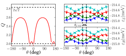
Any non-entangled state (including the steady state density matrix considered here) fulfills this inequality. A violation $Q>2$ is sufficient to prove entanglement. For a spin-singlet, a maximal $Q=2\sqrt{2}$ is obtained by orthogonal $\mathbf{a}_{K}\perp\mathbf{a}_{K^{\prime}}$, $\mathbf{b}_{K}\perp\mathbf{b}_{K^{\prime}}$, and $45^{\circ}$ between $\mathbf{a}_{K}$ and $\mathbf{b}_{K}$. Such optimal axes cannot be generally obtained in the CNT-CPS, for which $\mathbf{B}_{SOI}$ and $\theta_{CNT}$ are fixed by the sample fabrication, and only $\mathbf{B}$ is tunable. Yet, as we show in Fig. 2, this tunability is sufficient to obtain $Q>2$ as a function of the angle $\theta$ of a rotating in-plane field $\mathbf{B}=B(\sin\theta,0,\cos\theta)$ (see Fig. 1), for $B\sim|\mathbf{B}_{SOI}|$. The shown result is generic and we find similar $Q>2$ for most CNT chiralities, diameters, and QD lengths.

Realistic systems. In a realistic setup, the two QDs remain coupled through the superconducting region, their levels are broadened by the contacts, the splitting efficiency is imperfect and electron pairs can tunnel onto the same QD, the tunneling rates depend on the gate voltages, and electrons can interact. Any measurement probes the steady state density matrix $\rho$ of the full CPS system and not an ideal singlet state. The projections $P_{\pm a_{\tau}},P_{\pm b_{\tau^{\prime}}}$ are obtained by narrowing the measurement to an energy window capturing the electron transport through the corresponding level of each QD, typically by differential conductance measurements tuned to the resonances corresponding to the levels. The modified $\rho$ together with the measurement method leads to a distorted reconstruction of the spin correlators, and we need to distinguish between local and nonlocal distortion sources.

Local distortions in one QD are independent of the other QD and modify, e.g., $P_{\pm a_{\tau}}$ to $P_{+a_{\tau}^{\prime}},P_{-a_{\tau}^{\prime\prime}}$. We can write $P_{+a^{\prime}_{\tau}}-P_{-a^{\prime\prime}_{\tau}}=\gamma(\mathbf{S}\cdot\tilde{\mathbf{a}}_{\tau})+(1-\gamma)P_{\tilde{\mathbf{a}}_{\tau}}$ for an intermediate axis $\tilde{\mathbf{a}}_{\tau}$, $0\leq\gamma\leq 1$, and a remaining projection $P_{\tilde{\mathbf{a}}_{\tau}}$. The latter transforms any state into a product state, and local distortions therefore lower the ideal value of $Q$ by an amount set by the various $\gamma$ for the different QD levels. Assuming that the level broadening can be kept small so that there is only little overlap between nearby resonances (assisted also by a charging energy), the most important source of local distortions is disorder scattering within each QD. It mixes the wave functions in different valleys kuemmeth:2008 ; jespersen:2011 , and the $\left|\pm a_{\tau}\right\rangle$ are no longer the eigenstates. While of central importance in metallic CNTs, in semiconducting CNTs disorder scattering competes with the valley-preserving semiconducting gap of typically $\sim$ 100 meV, which has opposite signs in opposite valleys. If the disorder scattering amplitude is smaller it has a negligible influence. Therefore, semiconducting CNTs are preferable for testing the Bell inequality.

Valley mixing at injection, however, is essential. Indeed, if valleys and spins are correlated, for instance, if the singlet splits always into opposite valleys, the transport through other valley combinations does not provide any information on the Cooper pairs and the construction of $Q$ is no longer possible. For a valid spin correlator measurement the injection must mix valleys to produce a detectable signal through all resonances, yet the precise degree of mixing is unimportant.

Nonlocal distortions of the spin modify the spin projections as an effect of the entire CPS system, typically by hybridization between the two QDs, and the measured $P_{\pm a_{\tau}},P_{\pm b_{\tau^{\prime}}}$ become nonlocal operators. Such operators can generate additional entanglement through wave function mixing between the left and right QDs. In the CPS setup they are a source of error for detecting spin entanglement. Yet with the full microscopic calculation discussed next we can see that these nonlocal contributions can be kept under control in realistic conditions.

Figure 3: Results from the microscopic calculation of a CPS, based on a zigzag CNT of chirality (20,0) with a bending angle $\theta_{CNT}\approx 30^{\circ}$, in a field of $|\mathbf{B}|=0.5$ T (see the Supplemental Material supplement ). The SOI energies $\alpha=-0.10$ meV and $\beta=-0.40$ meV lead to $|\mathbf{B}|/|\mathbf{B}_{SOI}|\approx\mu_{B}g|\mathbf{B}|/2|\alpha-\beta|=0.10$. (a) Map of the conductance product $G_{L}G_{R}$ (units of $e^{4}/h^{2}$) as a function of QD gate voltages $V_{L,R}$ at $\theta=25^{\circ}$. The 4 levels of each QD give rise to the 4 resonances labeled by $\pm a_{\tau}$, $\pm b_{\tau^{\prime}}$. Inside the black squares, the CPS acts as a spin-valley filter for the projections $P_{\pm a_{\tau}}P_{\pm b_{\tau^{\prime}}}$, and integrating the signal within each black square yields the corresponding observable. (b) $V_{L,R}$ values marking the positions of the resonances of the levels $\pm a_{\tau}$ and $\pm b_{\tau^{\prime}}$ of the two QDs as a function of $\theta$. The curves are identical up to the shift by $\theta_{CNT}$. Levels in the same valley $\tau$ see the same field $\mathbf{B}^{\tau}_{\text{eff}}$ and are identified by having the same curvature as function of $\theta$. (c) $Q$ as a function of $\theta$ for the conductances $G$ given as subscripts of $Q$ in the figure legend. The $Q$ values are obtained by analyzing data as shown in panel (a) by the method described in the text. The yellow shaded region marks the allowed range of violation of the Bell inequality for the spin-singlets in the steady state.

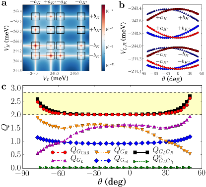
Microscopic model. To quantitatively access a realistic system and to determine the optimal choice of measurements that allows us to gain insight in the effects of local and nonlocal distortions, we have investigated a microscopic tight-binding model of the CNT-CPS. Our approach follows Ref. burset:2011, , which we have complemented to include magnetic fields by terms equivalent to Eq. (4) and valley mixing at injection. As a result, we obtain the partial conductances of the CPS due to Cooper pair splitting (crossed Andreev reflections, $G_{\text{CAR}}$), elastic cotunneling through the superconducting region ($G_{\text{EC}}$), and the local Andreev scattering contributions at each QD ($G_{\text{A}L},G_{\text{A}R}$). From these quantities, transport from the superconductor to the normal leads is expressed by the conductances $G_{j}=2(G_{\text{A}j}+G_{\text{CAR}})$ ($j=L,R$), and transport between the normal leads by the nonlocal conductance $G_{nl}=G_{\text{EC}}-G_{\text{CAR}}$.

In Fig. 3 (a) we display a conductance map for a semiconducting CNT as a function of the QD gate voltages $V_{L,R}$ that tune the QD levels to resonance. Such a result is useful for a Bell test if all 4 resonances in each QD are well resolved and their 16 points of intersection, corresponding to the products $P_{\pm a_{\tau}}\otimes P_{\pm b_{\tau^{\prime}}}$, form single peaks and not avoided crossings. To access this regime, we have chosen a coupling between the superconductor and the CNT on the order of the superconducting gap ($\lesssim$ 1 meV), and tuned the coupling to the leads such that the resonances are well resolved (see the Supplemental Material supplement ). Similar conditions have been obtained in experiments kuemmeth:2008 ; jespersen:2011 , and such a regime can be reached for a wide variety of samples and coupling strengths to the contacts.

To analyze the data we integrate the various conductances over regions centered at the crossings as shown by the black squares in Fig. 3 (a). From the resulting 16 integrals $G_{\pm a_{\tau},\pm b_{\tau^{\prime}}}$ we construct the spin correlators

$$C_{\mathbf{a}_{\tau},\mathbf{b}_{\tau^{\prime}}}=\frac{\sum_{\nu,\nu^{\prime}=\pm}\nu\nu^{\prime}G_{\nu a_{\tau},\nu^{\prime}b_{\tau^{\prime}}}}{\sum_{\nu,\nu^{\prime}=\pm}G_{\nu a_{\tau},\nu^{\prime}b_{\tau^{\prime}}}},$$ (6)

which is a simple consequence from the fact that $P_{+a_{\tau}}-P_{-a_{\tau}}=(\mathbf{S}\cdot\mathbf{a}_{\tau})$ and $P_{+a_{\tau}}+P_{-a_{\tau}}$ is the identity operator (see the Supplemental Material supplement ). From these $C_{\mathbf{a}_{\tau},\mathbf{b}_{\tau^{\prime}}}$ we determine $Q$ by Eq. (5), with the liberty of placing the $-$ sign in front of any term in Eq. (5) to obtain the maximum $Q$.

The Cooper pair splitting amplitude is directly described by $G_{\text{CAR}}$, and the corresponding curve $Q_{G_{\text{CAR}}}$ [Fig. 3 (c)] captures indeed a similar behavior as the ideal case of Fig. 2, with $Q>2$ in the $\theta$ regions where the levels of different valleys approach each other and the spin projections rotate [Fig. 3 (b)]. The measurable conductances $G_{j}$, however, contain with $G_{\text{A}j}$ contributions that represent strong enough local distortions to suppress $Q$ below 2. In the right QD the local distortions are enhanced by level overlaps close to $\theta=60^{\circ}$ where the $K$ and $K^{\prime}$ levels become degenerate [Fig. 3 (b)], and indeed $Q_{G_{R}}$ decreases in this region. In contrast, the left QD levels remain well separated, and $Q_{G_{L}}$ mirrors the upturn of $Q_{G_{\text{CAR}}}$, with $G_{\text{CAR}}$ overruling the $G_{\text{A}L}$ contribution. The same behavior with $G_{L}\leftrightarrow G_{R}$ is found near $\theta=-90^{\circ}$. On the other hand, $G_{nl}$ corresponds to an experiment of electron injection through a normal lead and contains with $G_{\text{EC}}$ a component describing the uncorrelated single-particle transport. Since we find that $G_{\text{EC}}$ and $G_{\text{CAR}}$ have a similar amplitude, we expect that $Q_{G_{nl}}\sim Q_{G_{\text{CAR}}}/2$. However, $G_{\text{EC}}$ contains also the higher order tunneling processes that represent the nonlocal distortions, which may cause $Q_{G_{nl}}$ to increase again. Nonetheless, we find that $Q_{G_{nl}}\sim 1$ with a similar shape as $Q_{G_{\text{CAR}}}$, indicating that the nonlocal distortions have a negligible effect.

While $G_{\text{CAR}}$ produces the purest indicator of spin entanglement, it is only indirectly accessible by experiments. On the other hand, the directly measurable $G_{j}$ are obscured by the local contributions of the $G_{\text{A}j}$. A method of circumventing this problem is to consider products of the $G_{j}$, such as $G_{L}G_{R}$. Since the projections $P\equiv P_{\pm a_{\tau}}\otimes P_{\pm b_{\tau^{\prime}}}$ eliminate all QD degrees of freedom, the product $G_{L}G_{R}$ is equivalent to a nonlocal current measurement with a density matrix $\rho^{\prime}$ whose nonlocal contribution is encoded in $P\rho^{\prime}P\propto P\rho^{2}P$. By the higher power of $\rho$ and the projections, the relative weight of the local contributions can be reduced, while a spin singlet in $P\rho P$ remains a spin singlet in $P\rho^{2}P$. In Fig. 3 (c) we see that the corresponding curve $Q_{G_{L}G_{R}}$ follows almost perfectly $Q_{G_{\text{CAR}}}$, showing that the multiplication $G_{L}G_{R}$ is powerful enough to suppress the local distortions in the $G_{j}$. Therefore, a high splitting efficiency of a CPS is not a primary requirement for the proposed Bell test.

To demonstrate that the large $Q$ value is indeed an effect of superconductivity, we show with $Q_{G_{L}G_{R}}^{n}$ the corresponding curve for $G_{L}G_{R}$ obtained for the normal state. The fact that $Q_{G_{L}G_{R}}^{n}\approx 0$ is the strongest indicator that $Q_{G_{L}G_{R}}$ demonstrates indeed the spin entanglement.

Finally, we have truncated the curves in Fig. 3 close to $\theta=60^{\circ}$ and $-90^{\circ}$ where QD levels strongly overlap [Fig. 3 (b)] and spin correlators can no longer be reconstructed. It is indeed important to maintain well separated QD levels. Hence the charging energy of the QDs, which has been neglected in the microscopic calculation, plays here an important role as it increases the level separation but has much reduced exchange coupling due to the SOI induced spin projections of the QD levels.

Conclusions. We have demonstrated that due to SOI effects bent CNT-CPS (or two CNTs under an angle) can be used for entanglement detection in the steady state by a violation of the Bell inequality. Notable for the Bell inequality is that the set of axes $\mathbf{a}_{\tau},\mathbf{b}_{\tau^{\prime}}$ along which the spin correlators must be measured can be arbitrary and the precise axis orientations, i.e., the precise SOI strengths, do not need to be known. This is an advantage over entanglement witnesses faoro:2007 or quantum state tomography. Although discussed for CNTs, the introduced concept of entanglement detection is general and can be implemented in any system allowing tunable spin-energy filtering. For an ideal CNT-CPS, a violation of the Bell inequality can be achieved for most CNTs over a large range of orientations of an external field $\mathbf{B}$ with strength $B\sim|\mathbf{B}_{SOI}|$, which for usual CNTs are $<1$ T. The robustness of this behavior was confirmed by a microscopic calculation that incorporates the local and nonlocal imperfections of a realistic system. From the results we propose the use of the product of conductances $G_{L}G_{R}$ as the optimal observable for testing the Bell inequality. We have furthermore argued that the spin reconstruction in semiconducting CNTs is robust against disorder.

To conclude, it should be noted that a bending of the CNT is not an absolute requisite. An equivalent effect can be obtained by applying individual $\mathbf{B}$ fields on the QDs or by providing a constant field offset on one QD by placing a ferromagnet in its vicinity, if sufficient control of the typical field strengths $|\mathbf{B}|\sim|\mathbf{B}_{SOI}|<1$ T can be granted. If two separate CNTs are connected to the superconductor, they should have similar diameters such that their $\mathbf{B}_{SOI}$ are comparable.

Acknowledgments. We thank A. Baumgartner, J. C. Budich, A. Cottet, N. Korolkova, P. Recher, and B. Trauzettel for helpful discussions and comments. We acknowledge the support by the EU-FP7 project SE2ND [271554] and by the Spanish MINECO through Grant No. FIS2011-26516. P.B. also acknowledges the support by the ESF under the EUROCORES Programme EuroGRAPHENE.

Supplemental Material

I Demonstration of Eq. (6)

The current flowing out of an ideal CPS originates only from split Cooper pairs, with one electron being transported over the left and one electron over the right QD. This current is, therefore, subjected to the filtering of spin, valley, and energy of both QDs, and probing the current locally in one QD contains the nonlocal information of the filtering effects of both QDs.

Indeed, in this situation, with filters set along the axes $\nu a_{\tau},\nu^{\prime}b_{\tau^{\prime}}$ ($\nu,\nu^{\prime}=\pm$) and resonant conditions such that transport is restricted to the selected levels, the density matrix for the outflowing particles takes the form $\rho_{\nu a_{\tau},\nu^{\prime}b_{\tau^{\prime}}}=P_{\nu a_{\tau}}P_{\nu^{\prime}b_{\tau^{\prime}}}\rho P_{\nu^{\prime}b_{\tau^{\prime}}}P_{\nu a_{\tau}}$, with $\rho$ the density matrix in the absence of spin-valley filtering. Due to the perfect splitting efficiency, the currents through the left and right QD are identical, and we can focus, for instance, on transport through the left QD only. If $\hat{I}_{L}$ is the spin and valley independent current operator for transport over the left QD, the property $[\hat{I}_{L},P_{\nu a_{\tau}}P_{\nu^{\prime}b_{\tau^{\prime}}}]=0$ ensures that $\langle\hat{I}_{L}\rangle=\mathrm{Tr}\{P_{\nu a_{\tau}}P_{\nu^{\prime}b_{\tau^{\prime}}}\hat{I}_{L}\rho P_{\nu^{\prime}b_{\tau^{\prime}}}P_{\nu a_{\tau}}\}=\mathrm{Tr}\{P_{\nu a_{\tau}}P_{\nu^{\prime}b_{\tau^{\prime}}}\hat{I}_{L}\rho\}$. In the linear response regime we have furthermore $\langle\hat{I}_{L}\rangle=VG_{L}$, with $G_{L}$ the conductance and $V$ the voltage applied to both leads with respect to the superconductor. As a function of both QD gate voltages, $G_{L}$ is resonant at the level crossing $\nu a_{\tau},\nu^{\prime}b_{\tau^{\prime}}$. The full amplitude of the transport at this level crossing, denoted by $G_{\nu a_{\tau},\nu^{\prime}b_{\tau^{\prime}}}$, is obtained by integrating $G_{L}$ over this resonance. If furthermore the tunneling rates to the QDs are independent of the QD gates, the quantities $\langle P_{\nu a_{\tau}}P_{\nu^{\prime}b_{\tau^{\prime}}}\rangle=G_{\nu a_{\tau},\nu^{\prime}b_{\tau^{\prime}}}/\sum_{\tilde{\nu},\tilde{\nu}^{\prime}}G_{\tilde{\nu}a_{\tau},\tilde{\nu}^{\prime}b_{\tau^{\prime}}}$ allow us to reconstruct the spin correlators due to the identites $(P_{+a_{\tau}}-P_{-a_{\tau}})\otimes(P_{+b_{\tau^{\prime}}}-P_{-b_{\tau^{\prime}}})=(\mathbf{S}\cdot\mathbf{a}_{\tau})\otimes(\mathbf{S}\cdot\mathbf{b}_{\tau^{\prime}})$ and $(P_{+a_{\tau}}+P_{-a_{\tau}})\otimes(P_{+b_{\tau^{\prime}}}+P_{-b_{\tau^{\prime}}})=\openone\otimes\openone$. As a consequence we obtain Eq. (6) in the main text. The relation between conductances and spin correlators, therefore, follows from the same considerations used in the proposed entanglement tests based on noise measurements Scps ; Sbell_solid_state .

To further test Eq. (6) and its consequences on entanglement detection under realistic conditions, we have implemented the microscopic numerical calculation. As discussed in the main text, the numerical results give an objective demonstration that Eq. (6) and the conclusions for entanglement detection remain robust.

II Influence of realistic setup on $Q$

In this part of the supplement we illustrate the influence of the coupling of the CNT to the superconductor and the normal leads on the determination of $Q$. We provide all parameters used for the tight-binding calculation following Ref. Sburset:2011, . Finally we show how the level energies and the spin projections evolve with the magnetic field.

Figure S1 shows the dependence of $Q$ on the effective coupling strength $\Gamma_{S}$ between the superconductor and the CNT. The insets show parts of the conductance maps for the $\Gamma_{S}$ values corresponding roughly to the placements of the insets in the plot. For large $\Gamma_{S}$, the level broadening induced by the superconducting contact mixes the Cooper pairs between the QD levels and the conductances are no longer spin projective. This is notable by the similar intensities of all resonances, and corresponds to a strong enhancement of the local distortions discussed in the text. The corresponding values of $Q$ lie well below $2$. Small $\Gamma_{S}$, on the other hand, lead to a weak Cooper pair injection amplitude compared with the hybridization through the superconducting region. As a consequence, the resonance crossings turn into anticrossings. The resulting $Q$ values sharply increase beyond $Q=2\sqrt{2}$ due to strongly distorted spin correlator reconstructions by the nonlocal hybridization processes. At very small $\Gamma_{S}$, the anticrossings of different levels overlap, and the spin correlator reconstruction becomes erratic.

Figure S1: Dependence of $Q$ on the effective coupling $\Gamma_{S}$ to the superconductor for a (20,0) CNT with fixed $\Gamma_{L,R}=27$ meV, $B=0.5$ T, $\theta=45^{\circ}$, $\theta_{CNT}=28.8^{\circ}$. The insets show a zoom on the conductance maps for the $\Gamma_{S}$ values corresponding to their placement in the figure, with identical logarithmic color scales [see Fig. 3 (a) in the main text]. The center inset represents the valid regime for testing the Bell inequality with well resolved resonances of different intensities, and the absence of notable avoided crossings of the resonance peaks.

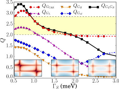
A valid measurement of $Q$ requires $\Gamma_{S}$ corresponding to the central inset in the Fig. S1, represented by well-defined level crossing peaks with unequal intensities. The unequal intensities are a result from the spin filtering of the singlet states, such that spin projection axes that are close to parallel suppress the conductance, while projections that are close to antiparallel allow a maximal transmission. Hence unequal, $\theta$ dependent peak intensities are a necessary indicator for spin entanglement, and indeed are the basis for the implementation of the Bell test.

The dependence on the tunnel coupling to the normal leads, characterized by a tunneling amplitude $\Gamma_{j}$ for $j=L,R$, is represented in Fig. S2. The combination of the $\Gamma_{j}$ with $\Gamma_{S}$ defines the broadening of the QD levels. Indeed, in the model of Ref. Sburset:2011, the lateral leads were represented by ideal one-dimensional channels weakly coupled to each end site of the nanotube. In the present calculations the tunneling rates to these leads $\Gamma_{j}$ take values between 10 and 100 meV. The actual broadening introduced to the QD levels becomes then on the order of $\Gamma_{j}a/W_{j}$ with $W_{j}$ the length of QD $j$ and $a$ the lattice constant.

Figure S2: Dependence of $Q$ on the tunneling amplitudes $\Gamma_{j}$ to the normal lead $j=L,R$, for $\Gamma_{L}=\Gamma_{R}$ for a (20,0) CNT with fixed $\Gamma_{S}=1.35$ meV, $B=0.5$ T, $\theta=45^{\circ}$, $\theta_{CNT}=28.8^{\circ}$. The insets show a zoom on the conductance maps for the $\Gamma_{j}$ values corresponding to their placement in the figure, with identical logarithmic color scales [see Fig. 3 (a) in the main text]. The center inset represents the valid regime for testing the Bell inequality with well separated resonances and a high enough pixel resolution such that the integral weight of each peak can be determined with high accuracy.

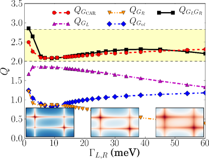
In contrast to $\Gamma_{S}$, the insets in Fig. S2 show that $\Gamma_{j}$ contributes only to a broadening of the levels but leaves the inequality of the peaks unchanged. The $\Gamma_{j}$ values of the insets correspond again roughly to the positions of the insets. At large $\Gamma_{j}$, the level overlaps lead to strong local overlaps of the projections such that the $Q_{G_{j}}$ strongly decrease. Since, however, the unequal intensities and so the spin-filtering properties of each QD level are maintained, the value of $Q_{\text{CAR}}$ remains large even for large $\Gamma_{j}$. Yet for larger $\Gamma_{j}$ the influence of the overlaps is well notable by the split off of $Q_{G_{L}G_{R}}$ from the $Q_{\text{CAR}}$ value. For small $\Gamma_{j}$ we notice that most conductances lead to an upturn of $Q$. This effect is attributable to the finite resolution of the peaks from the numerics that become only a few pixels wide, and the result is strongly susceptible to the discretization steps of the $V_{j}$. The artificial nature of the low $\Gamma_{j}$ behavior is indeed seen by the comparison of $Q_{G_{L}}$ and $Q_{G_{R}}$, which show an anomalous opposite behavior in a regime where all resonances are well separated and all couplings to the left and right QDs are identical. Finally, we notice that since the $\Gamma_{j}$ mainly influence the QD levels locally, an asymmetry $\Gamma_{L}\neq\Gamma_{R}$ has only little impact on the value of $Q$ as long as all levels can be well resolved.

The results shown in the main text represent the optimal values for the chosen CNT and geometry, $\Gamma_{S}=1.35$ meV and $\Gamma_{L}=\Gamma_{R}=27$ meV, determined by first identifying a valid $\Gamma_{S}$ leading to well shaped peaks with modulated intensities, and then optimizing the $\Gamma_{j}$ to obtain well resolved resonances. These values, however, are strongly sample and geometry dependent and can be used only as indicative.

For the present calculation we have used a CNT of chirality (20,0) with QD lengths $W_{L}=W_{R}=43$ nm and a length of the central superconducting region of 173 nm. Yet the same behavior of level separations and $Q$ values is found for longer system sizes corresponding to experimental situations. A magnetic field of strength $B=0.5$ T was applied to each QD region with angles $\theta$ on the left QD and angles $\theta+\theta_{CNT}$ on the right QD with respect to the CNT axis, for $\theta_{CNT}=28.8^{\circ}$. The SOI strengths $\alpha,\beta$ and the shift $\Delta k^{cv}_{t}$ have been implemented using the values of Refs. Sklinovaja:2011a, ; Sklinovaja:2011b, , and are given by $\alpha=-0.08$ meV $/R$, $\beta=-0.31$ meV $\cos(3\eta)/R$, and $\hbar v_{F}\Delta k^{cv}_{t}=-5.4$ meV $\tau\cos(3\eta)/R^{2}$ with $R$ the CNT radius in nm, $\tau=K,K^{\prime}=+,-$, and $\eta$ the chiral angle, $\tan(\eta)=\sqrt{3}N_{2}/(2N_{1}+N_{2})$, for a CNT with chiralities $(N_{1},N_{2})$. For $(N_{1},N_{2})=(20,0)$ we have $R=0.78$ nm, $\alpha=-0.10$ meV, and $\beta=-0.40$ meV. The induced superconducting gap is $\Delta=0.1$ meV, and the doping of the central region $-243$ meV. All further parameters are as described in Ref. Sburset:2011, . For $(N_{1},N_{2})=(18,10)$ as used for Fig. 2 in the main text, we have $R=0.96$ nm, $\alpha=-0.08$ meV, and $\beta=-0.15$ meV.

Figure S3: Levels and spin projections of the left QD as a function of parallel and perpendicular magnetic fields $B$ for the (18,10) CNT described in Fig. 2 of the main text. The sketches in the lower left corners indicate the $B$ field directions with respect to the left QD. The arrows indicate the spin projections in the $(x,z)$ plane with the $S^{z}$ direction pointing upwards and the $S^{x}$ direction to the right in the plots. At $B=0$ the levels of both valleys are degenerate. At increasing $B$, the levels of one valley increase and the levels of the other valley decrease in energy by the combined effect of orbital and Zeeman fields. At parallel field, the spins remain parallel to the CNT axis. At perpendicular field, the level energies are only weakly affected by $B$, yet the spin projections in each valley strongly rotate. The situations at $B=0.4$ T correspond to the selected angles $\theta=0^{\circ}{},90^{\circ}{}$ in the upper right panel of Fig. 2 in the main text.

Figure S4: Levels and spin projections as in Fig. S3 for the right QD at the angle $\theta_{CNT}=30^{\circ}$ to the left QD. The sketches in the lower left corners indicate the $B$ field directions with respect to the right QD. The spins are shown in the global $(x,z)$ basis corresponding to Fig. S3. The situations at $B=0.4$ T correspond to the selected angles $\theta=0^{\circ}{},90^{\circ}{}$ in the lower right panel of Fig. 2 in the main text.

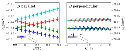
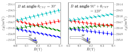
Finally, we illustrate the evolution of the QD levels and their spin polarizations as a function of the magnetic field $B$. Figure S3 displays the 4 spin polarized QD levels of the (18,10) CNT model used for Fig. 2 in the main text, for magnetic fields parallel and perpendicular to the CNT axis of the left QD, respectively. Figure S4 shows the levels of the right QD for the same fields, which are seen for this QD under the additional angle $\theta_{CNT}=30^{\circ}$.

References

- (1) P. Recher, E. V. Sukhorukov, and D. Loss, Phys. Rev. B 63, 165314 (2001).
- (2) G. B. Lesovik, T. Martin, and G. Blatter, Eur. Phys. J. B 24, 287 (2001); S. Kawabata, J. Phys. Soc. Jpn. 70, 1210 (2001).
- (3) L Hofstetter, S. Csonka, J. Nygård, and C. Schönenberger, Nature (London) 461, 960 (2009).
- (4) L. G. Herrmann, F. Portier, P. Roche, A. Levy Yeyati, T. Kontos, and C. Strunk, Phys. Rev. Lett. 104, 026801 (2010).
- (5) L Hofstetter, S. Csonka, A. Baumgartner, G. Fülöp, S. d’Hollosy, J. Nygård, and C. Schönenberger, Phys. Rev. Lett. 107, 136801 (2011).
- (6) A. Das. Y. Ronen, M. Heiblum. D. Mahalu, A. V. Kretinin, and H. Shtrikman, Nature Commun. 3, 1165 (2012).
- (7) J. Schindele, A. Baumgartner, and C. Schönenberger, Phys. Rev. Lett. 109, 157002 (2012).
- (8) An alternative consisting in transferring signatures of electron entanglement to photons is discussed in A. Cottet, T. Kontos, and A. Levy Yeyati, Phys. Rev. Lett. 108, 166803 (2012).
- (9) J. F. Clauser, M. A. Horne, A. Shimony, and R. A. Holt, Phys. Rev. Lett. 23, 880 (1969).
- (10) N. M. Chtchelkatchev, G. Blatter, G. B. Lesovik, T. Martin, Phys. Rev. B 66, 161320(R) (2002); P. Samuelsson, E.V. Sukhorukov, and M. Büttiker, Phys. Rev. Lett. 91, 157002 (2003).
- (11) The steady state entanglement test proposed in this work has to be distinguished from a single pair detection such as in Aspect’s experiments [A. Aspect, J. Dalibard, and G. Roger, Phys. Rev. Lett. 49, 1804 (1982)].
- (12) W.-R. Hannes and M. Titov, Phys. Rev. B 77, 115323 (2008).
- (13) M. Veldhorst and A. Brinkman, Phys. Rev. Lett. 105, 107002 (2010).
- (14) W. Izumida, K. Sato, and R. Saito, J. Phys. Soc. Jpn. 78, 074707 (2009).
- (15) J.-S. Jeong and H.-W. Lee, Phys. Rev. B 80, 075409 (2009).
- (16) J. Klinovaja, M. J. Schmidt, B. Braunecker, and D. Loss, Phys. Rev. Lett. 106, 156809 (2011).
- (17) J. Klinovaja, M. J. Schmidt, B. Braunecker, and D. Loss, Phys. Rev. B 84, 085452 (2011).
- (18) D. V. Bulaev, B. Trauzettel, and D. Loss, Phys. Rev. B 77, 235301 (2008).
- (19) S. Weiss, E. I. Rashba, F. Kuemmeth, H. O. H. Churchill, and K. Flensberg, Phys. Rev. B 82, 165427 (2010).
- (20) J. S. Lim, R. López, and R. Aguado, Phys. Rev. Lett. 107, 196801 (2011).
- (21) F. Kuemmeth, S. Ilani, D. C. Ralph, and P. L. McEuen, Nature (London) 452, 448 (2008).
- (22) T. S. Jespersen, K. Grove-Rasmussen, K. Flensberg, J. Paaske, K. Muraki, T. Fujisawa, and J. Nygård, Phys. Rev. Lett. 107, 186802 (2011).
- (23) P. Burset, W. Herrera, and A. Levy Yeyati, Phys. Rev. B 84, 115448 (2011).
- (24) See Supplemental Material for more details.
- (25) L. Faoro and F. Taddei, Phys. Rev. B 75, 165327 (2007).
- (1) G. B. Lesovik, T. Martin, and G. Blatter, Eur. Phys. J. B 24, 287 (2001); S. Kawabata, J. Phys. Soc. Jpn. 70, 1210 (2001).
- (2) N. M. Chtchelkatchev, G. Blatter, G. B. Lesovik, T. Martin, Phys. Rev. B 66, 161320(R) (2002); P. Samuelsson, E.V. Sukhorukov, and M. Büttiker, Phys. Rev. Lett. 91, 157002 (2003).
- (3) P. Burset, W. Herrera, and A. Levy Yeyati, Phys. Rev. B 84, 115448 (2011).
- (4) J. Klinovaja, M. J. Schmidt, B. Braunecker, and D. Loss, Phys. Rev. Lett. 106, 156809 (2011).
- (5) J. Klinovaja, M. J. Schmidt, B. Braunecker, and D. Loss, Phys. Rev. B 84, 085452 (2011).