Universality in modelling non-equilibrium pattern formation in polariton condensates

Abstract

The key to understanding the universal behaviour of systems driven away from equilibrium lies in the common description obtained when particular microscopic models are reduced to order parameter equations. Universal order parameter equations written for complex matter fields are widely used to describe systems as different as Bose-Einstein condensates of ultra cold atomic gases, thermal convection, nematic liquid crystals, lasers and other nonlinear systems. Exciton-polariton condensates recently realised in semiconductor microcavities are pattern forming systems that lie somewhere between equilibrium Bose-Einstein condensates and lasers. Because of the imperfect confinement of the photon component, exciton-polaritons have a finite lifetime, and have to be continuously re-populated. As photon confinement improves, the system more closely approximates an equilibrium system. In this chapter we review a number of universal equations which describe various regimes of the dynamics of exciton-polariton condensates: the Gross-Pitaevskii equation, which models weakly interacting equilibrium condensates, the complex Ginsburg-Landau equation—the universal equation that describes the behaviour of systems in the vicinity of a symmetry–breaking instability, and the complex Swift-Hohenberg equation that in comparison with the complex Ginsburg-Landau equation contains additional nonlocal terms responsible for spacial mode selection. All these equations can be derived asymptotically from a generic laser model given by Maxwell-Bloch equations. Such an universal framework allows the unified treatment of various systems and continuously cross from one system to another. We discuss the relevance of these equations, and their consequences for pattern formation.

0.1 Introduction

For a dissipative macroscopic system in thermal equilibrium, relaxation toward a state of minimum free energy determines the states that the system may adopt, and any possible pattern formation. In contrast, if a system is driven out of equilibrium by external fluxes, then no such simple description is possible. i.e., if a system may exchange particles and energy with multiple baths (reservoirs), then the states the system adopts depend not only on the temperatures and chemical potentials of these reservoirs, but also on the rate at which particles and energy are injected and lost from the system. This can not generally be captured by relaxation to minimise a given energy functional

Both equilibrium and non-equilibrium systems can be characterised by mean-field variables if field fluctuations are negligible (fluctuations can however be introduced phenomenologically into the evolution equations if required). A mean-field approach leads naturally to the concept of the order parameter, and the corresponding order parameter equation. The order parameter is either a physical field or an abstract field which acquires a non-zero value in the an ordered phase (such as a Bose-condensed or lasing state), and vanishes in the normal state. When considering a spatially inhomogeneous system (with trapping, or inhomogeneous pumping), the order parameter may vary in space. When considering a non-equilibrium system, or the dynamics of a system as it approaches its equilibrium state, the order parameter may also vary in time. In such cases, the order parameter equation describes the space and time dependence of the order parameter, accounting for the generic features of the system’s dynamics.

One important classification of order parameter equations distinguishes whether they describe relaxation towards an equilibrium configuration, or phase evolution in a conservative system, or a mixture of the twoPismenBook:1999 . For a dissipative system, the dynamics may be described by using an energy functional $\mathcal{F}[\psi]$, written in terms of the order parameter $\psi$ and its spatial derivatives. The dissipative system dynamics causes this energy functional to decay as a function of time, reaching a minimal value at equilibrium, i.e. $\partial_{t}\psi=-\Gamma\partial_{\psi}\mathcal{F}$. The dynamical critical behaviour of such systems has been extensively reviewed by Hohenberg and Halperin Hohenberg:1977 . Such an approach is appropriate for many solid-state systems, including in particular non-equilibrium superconductivity kopnin:2001 . In contrast, for isolated systems such as ultracold atomic gases, the order parameter obeys conservative dynamics, in which the energy functional does not change with time, and the order parameter instead follows Hamiltonian dynamics. We will discuss the behaviour of systems that lie between these two extremes of purely dissipative and purely conservative dynamics, a scenario that includes the non-equilibrium polariton condensate.

The structure of the energy functional, and thus of the resulting order parameter equation, is determined by the symmetries of the order parameter space. Taking into account also the fact that near a phase transition, the characteristic lengthscale of fluctuations diverges, it becomes possible to restrict the form of the energy functional by keeping the lowest order derivative terms that possess the required symmetries. This makes it possible to divide systems into universality classes, depending only on the symmetries and the nature of the dynamics Hohenberg:1977 ; kadanoff:2000 . Identifying which classes various system belong to allows one to draw similarities between systems that are very different in nature and to predict the behaviour of the new systems that fall into previously known universality class. For instance, symmetry under changing the phase of of the order parameter restricts the energy functionals to dependence on $|\psi|$ only, and considering the lowest order form that allows for a symmetry breaking from disordered (zero) to ordered (nonzero) state gives a potential as a quartic polynomial in $|\psi|$. Including the lowest compatible order of spatial derivative terms then gives the energy functional whose dissipative dynamics correspond to the Ginzburg-Landau equation:

$${\cal{F}}=\int dV\nabla\psi\cdot\nabla\psi^{*}+(\mu-U_{0}|\psi|^{2})^{2},$$ (1)

where $\mu$ is the control parameter that forces the system to move from the normal state $|\psi|=0$ to the ordered state with $|\psi|^{2}=\mu/U_{0}$. Eq. (1) is expected to be relevant to a physical system in the vicinity of the phase transition, where the smallness of the modulus and the derivatives of the order parameter allow to keep only the leading order terms in the expansion. Higher derivatives and other higher order terms can be kept to allow for more complex forms of order and associated phase transitions.

Understanding the universality class of a given system leads to understanding of fundamentals of the behaviour of that system. The studies of vortices and vortex dynamics in superfluid helium Hall:1956eh led to prediction and experimental realisation of vortices first in nonlinear optics Arecchi:1991jw , then in atomic Bose-Einstein condensates Dodd:1997cj and finally in nonequilibrium solid-state condensates Liew:2007kn ; Lagoudakis:2008ia all due the hydrodynamic interpretation of the order parameter equations. Spiral waves in biological and chemical systems suggested the existence of such meandering waves in class B lasers. Solitary waves in atomic systems all have their analogs in nonlinear optics. Finally, much of the experiments in solid-state condensates are now motivated by finding localised excitations similar to other system that share the same universality class Amo:2011bfa ; Dzyapko:2010tf . Pattern formation in systems that belong to the same universality class share similar properties. Patterns appear in open nonlinear systems when an amplitude distribution of the order parameter becomes unstable above a certain threshold. Linear instability gives rise to a so-called pure state that, if nonlinearities are weak, can dominate the dynamics. Strong nonlinearities may mix the eigenvalues leading to various stationary or chaotic combinations of pure states with different combinations occupying either all space or different space regions.

In this chapter we shall follow the evolution from equilibrium condensates to non-equilibrium condensates to lasers analysing their universality, emphasising similarities and differences. We will discuss in some detail the origin of the most general order parameter equation for the laser system, and comment on the relation of this order parameter equation to that for cold atoms and for non-equilibrium polariton condensation. We will then demonstrate how the various terms that may exist in the order parameter equation affect the patterns which arise, focusing on three cases: the case with homogeneous pumping and no trapping, the case with inhomogeneous pumping and no trapping, and the case with an harmonic trap.

0.1.1 Review of physical systems

Laser dynamics is described by coupling Maxwell equations with Shrödinger equations for $N$ atoms confined in the cavity. Expanding the electric field in cavity modes and keeping only the leading order mode leads to the equations that couple the amplitude of this mode with the collective variables that describe the polarisation and population of the gain medium. Such coupled equations are known as Maxwell-Bloch (MB) equations. Lasers are then classified depending on the relative order of the loss rates for the electric field, compared to the decay rates of the gain medium polarisation and population. The MB equations have two homogeneous stationary solutions: nonlasing (zero order parameter) and lasing (nonzero order parameter) solutions. The instabilities of these solutions, and therefore, pattern formation, are described by universal order parameter equations: the complex Swift-Hohenberg (cSH) equation for lasers with a fast population inversion and the cSH equation coupled to a mean flow if the population inversion is slowly varying. The universal equation describing the bifurcation of lasing solution takes the form of a cSH equation coupled to a Kuramoto-Sivashinsky equation Kuramoto:1976 ; Sivashinsky:1977 .

Semiconductor microcavities confine photon modes, which may then interact with electronic excitations in the semiconductor. If the cavity is resonant with the energy to create an exciton (a bound electron hole pair), and if the exciton-photon coupling is strong enough, then new normal modes (new quasiparticles) arise as hybrids of excitons and photons: polaritons. For low enough densities, these may be considered as bosonic quasiparticles, and so can form a condensed (coherent) state above a critical density. These are intrinsically non equilibrium systems with the steady states set by balance between pumping and losses due to the short lifetime of polaritons. Depending on whether the emission from the microcavity follows the bare photon or the lower polariton dispersion the system shows either regular lasing or polariton condensation and in this sense crosses over continuously from weak coupling at higher temperatures and pumping strengths to strong coupling at lower temperatures and lower pumping intensities. Losses in the microcavity systems can be decreased by improving the quality of dielectric Bragg mirrors. The smaller the pumping and losses become the closer polariton condensates come to resemble equilibrium Bose-Einstein condensates (BECs). It seems therefore that the unified approach should be possible to describe the transition from normal lasers to the equilibrium BECs via polariton condensates. There are some other differences between atomic or polariton condensates and normal lasers. The operation of a photon laser is based on three ingredients: a resonator for the electromagnetic field, an gain medium and a excitation mechanism for the gain medium. When excited, the gain medium will undergo stimulated emission of radiation that amplifies the electromagnetic field in the cavity. In contrast, for polariton condensates there is instead stimulated scattering within the set of polariton modes, and condensation can take place without any inversion of the gain medium, and thus potentially having a lower threshold Imamoglu:1996vwa . A microscopic theory would be required to fully describe how all of these aspects cross over from polariton condensation to lasing, however given the universality of order parameter equations, one may hope to write a single order parameter equation which captures these different regimes by varying appropriate parameters.

0.2 Derivation of order parameter equations

In this section we show how various order parameter equations arise in descriptions of lasers, and how these relate to the order parameter equations relevant to ultracold atoms and polariton condensates. We start with a mean field (semiclassical) model of a laser, the MB system of equations. In section 0.2.2 we show how the assumption of small relaxation times for atomic polarisation in comparison with the cavity relaxation time reduces these equations to the complex Ginzburg-Landau (cGL) equations Aranson:2002kba or the coupled cGL equation and the gain medium population dynamics Taranenko:1997bt . These models have been extensively used to model non-equilibrium condensates Dzyapko:2010tf ; Wouters:2010gwb ; Keeling:2008hj ; Wouters:2007dia . We discuss how the mode selection, in which a particular transverse mode grows fastest, is lost in the derivation of these models. Then, in Sec. 0.2.3 we instead follow the derivation used in Moloney:1995usa based on the multi-scale expansion technique to derive the cSH equations for class A and class C lasers Cross:1993ela . In section 0.2.4 we then discuss how nonlinear interactions appear in these equations, and discuss the interpretation of these equations as order parameter equations for polariton condensates. If the reservoir dynamics is slow in comparison with time evolution of the order parameter these equation should be replaced by a coupled system explicitly modelling the reservoir dynamics. In the limit of the long life-time of the particles the system becomes the Gross-Pitaevskii (GP) equation aka the nonlinear Schrödinger (NLS) equation that describes atomic BECs.

0.2.1 Maxwell-Bloch equations for a laser

We start with the MB equations for a wide-aperture laser with an intracavity saturable absorber with multiple transverse modes in the single longitudinal mode approximation Lugiato:1988bta

$$\frac{\partial E}{\partial t}-i\nabla^{2}E=P_{g}-P_{a}-(1+i\Delta_{e})E,$$ (2)

$$\tau_{\perp g}\frac{\partial P_{g}}{\partial t}+(1+i\Delta_{g})P_{g}=EG,$$ (3)

$$\tau_{\perp a}\frac{\partial P_{a}}{\partial t}+(1+i\Delta_{a})P_{a}=EA,$$ (4)

$$\tau_{g}\frac{\partial G}{\partial t}=G_{0}-G-\frac{1}{2}(E^{*}P_{g}+EP_{g}^{*}),$$ (5)

$$\tau_{a}\frac{\partial A}{\partial t}=A_{0}-A-\frac{D}{2}(E^{*}P_{a}+EP_{a}^{*}),$$ (6)

where the complex field $E$ is the envelope of the electric field, the real functions $G$ and $A$ are the population differences for gain and absorption media, the complex functions $P_{g}$ and $P_{a}$ are the envelopes of polarisation for gain and absorption media. $G_{0}$ and $A_{0}$ are the stationary values of the population difference in the absence of the laser field; they are proportional to the external gain and losses in the system.The parameter $D=\tau_{\perp a}\tau_{a}\mu_{a}^{2}/(\tau_{\perp g}\tau_{g}\mu_{g}^{2})$ is the relative saturability of gain and loss media and $\mu_{a}$ and $\mu_{g}$ stand for the atomic dipole momenta. The parameters $\tau_{\perp a,g}$ and $\tau_{a,g}$ are the relaxation times for atomic polarisations and population differences scaled by the cavity relaxation time, the time $t$ is also scaled by the cavity relaxation time. The parameters $\Delta_{a}-\Delta_{e}=(\omega_{a}-\omega_{c})\tau_{\perp a}$ and $\Delta_{g}-\Delta_{e}=(\omega_{g}-\omega_{c})\tau_{\perp g}$ are detunings between the spectral line centre and the frequency of empty cavity mode $\omega_{c}$. Without loss of generality we work in rotating frame such that the the fast time is eliminated via introduction of $\Delta_{e}$. The spatial coordinates are rescaled by the width of the effective Fresnel zone.

0.2.2 Fast reservoir dephasing limit

Following Staliunas:1993fk ; Fedorov:2000uja we assume that $\tau_{\perp a},\tau_{\perp g}$ are small and consider the first-order approximations to Eqs. (2-6). Keeping up to the linear terms in these small quantities we get

$$P_{g}=\frac{GE}{1+i\Delta_{g}}-\tau_{\perp g}\frac{(GE)_{t}}{(1+i\Delta_{g})^{2}},$$ (7)

and similar for $P_{a}$. The equation on $E$ after we substitute these expressions for $P_{g}$ and $P_{a}$ becomes

$$(1+i\eta)\frac{\partial e}{\partial t}-i(\nabla^{2}-\Delta_{e})e=[(1-i\Delta_{g})g-(1-i\Delta_{a})a-1]e,$$ (8)

where

$$\eta=-2\tau_{\perp g}g\Delta_{g}/(1+\Delta_{g}^{2})+2\tau_{\perp a}a\Delta_{a}/(1+\Delta_{a}^{2}),$$ (9)

and where we rescaled fields as $e=E/(1+\Delta_{g}^{2}),g=G/(1+\Delta_{g}^{2})$ and $a=A/(1+\Delta_{a}^{2})$. In writing Eq. (8) we kept leading order contributions in the imaginary coefficient of time derivative (which is of order $O(\tau_{\perp g},\tau_{\perp a})$). The real coefficient of the time derivative we kept to $O(1)$ in $\tau_{\perp g}$ and $\tau_{\perp a}$. The equations for scaled gain and absorption media populations to leading order take the forms:

$$\tau_{g}\frac{\partial g}{\partial t}=g_{0}-(1+|e|^{2})g,$$ (10)

$$\tau_{a}\frac{\partial a}{\partial t}=a_{0}-(1+d|e|^{2})a,$$ (11)

where $a_{0}=A_{0}/(1+\Delta_{a}^{2}),g_{0}=G_{0}/(1+\Delta_{g}^{2})$ and $d=D(1+\Delta_{g}^{2})/(1+\Delta_{a}^{2})$.

Fast reservoir population relaxation

The system of equations (8, 10, 11) can be simplified under more stringent restrictions on parameters. In the limit of fast population relaxation times $\tau_{g},\tau_{a}\ll 1$ (class A and C lasers) Eqs.( 10, 11) give

$$g=\frac{g_{0}}{1+|e|^{2}},\qquad a=\frac{a_{0}}{1+d|e|^{2}},$$ (12)

and Eq. (8) becomes

$$(1+i\eta(e))\frac{\partial e}{\partial t}-i\nabla^{2}e=\biggl{[}\frac{(1-i\Delta_{g})g_{0}}{1+|e|^{2}}-\frac{(1-i\Delta_{a})a_{0}}{1+d|e|^{2}}-1\biggr{]}e,$$ (13)

where the coefficient $\eta$ is given by

$$\eta(e)=-2\biggl{[}\frac{\tau_{\perp g}g\Delta_{g}}{(1+\Delta_{g}^{2})(1+|e|^{2})}-\frac{\tau_{\perp a}a\Delta_{a}}{(1+\Delta_{a}^{2})(1+d|e|^{2})}\biggl{]}.$$ (14)

Close to the emission threshold $|e|^{2}\ll 0$, which allows a cubic approximation for the nonlinear terms we get the complex Ginsburg-Landau equation (cGL) Aranson:2002kba

$$(i-\eta(0))\frac{\partial e}{\partial t}=-\nabla^{2}e+Ve+U|e|^{2}e+i[\alpha-\beta|e|^{2}]e,$$ (15)

where we let $\alpha=g_{0}-a_{0}-1$, $\beta=g_{0}-a_{0}$, $U=da_{0}\Delta_{a}-g_{0}\Delta_{g}$ , $V=g_{0}\Delta_{g}-a_{0}\Delta_{a}$.

The cGL equation is not a very accurate model of a laser since it does not take into account the selection of transverse modes. The lasers emit particular transverse modes that depend on the length of the resonator. By making the assumption that $\tau_{\perp g},\tau_{\perp a}\rightarrow 0$, we assumed that the gain line is infinitely broad. In order to take into account the tunability of lasers that allows spatial-frequency selection a more careful derivation of the order parameter equation is required, which does not take this limit of fast polarisation relaxation.

0.2.3 Multi-scale analysis of the Maxwell-Bloch equations

In this section we derive the complex Swift-Hohenberg equation capable of selecting particular transverse modes from the MB Eqs. (2–6). A similar derivation has been done for the MB equations taking into account gain only and assuming that $\Delta_{g}$ is small Lega:1994kaa . Here we shall only assume that $\nabla^{2}-\Delta_{e}$ is small and use it as a small parameter, $\epsilon(\nabla^{2}-\Delta_{e})$. We apply the technique of multi-scale expansion to $E,P_{g,a},G$ and $A$ looking for solutions in the form of a power series expansion in $\epsilon$, and introducing two slow time scales $T_{1}=\epsilon t$, $T_{2}=\epsilon^{2}t$, so that $\partial_{t}=\epsilon\partial_{T_{1}}+\epsilon^{2}\partial_{T_{2}}$. Next we solve equations at equal powers of $\epsilon$. At the leading order we get non-lasing solution $(E,P_{g},P_{a},G,A)=(0,0,0,G_{0},A_{0})$. At $O(\epsilon)$, $(E_{1},P_{g1},P_{a1},G_{1},A_{1})=(\psi,G_{0}\psi/(1+i\Delta_{g}),A_{0}\psi/(1+i\Delta_{a}),0,0)$, where $\psi$ is a yet undetermined complex field and $G_{0}$ and $A_{0}$ are linked via $1=G_{0}/(1+i\Delta_{g})-A_{0}/(1+i\Delta_{a})$. This condition specifies $G_{0}$ and $A_{0}$ at the threshold for laser emission as $G_{\text{crit}}=\Delta_{a}(1+\Delta^{2}_{g})/(\Delta_{a}-\Delta_{g})$ and $A_{\text{crit}}=\Delta_{g}(1+\Delta^{2}_{a})/(\Delta_{a}-\Delta_{g})$. We make near-threshold assumption $G_{0}=G_{\text{crit}}+\epsilon^{2}l_{g}$ and $A_{0}=A_{\text{crit}}+\epsilon^{2}l_{a}$. At $O(\epsilon^{2})$ we get

$$\frac{\partial\psi}{\partial T_{1}}=i(\nabla^{2}-\Delta_{e})\psi+P_{g2}-P_{a2}-E_{2},$$ (16)

$$\tau_{\perp g}\frac{\partial P_{g1}}{\partial T_{1}}+(1+i\Delta_{g})P_{g2}=E_{2}G_{0},$$ (17)

$$\tau_{\perp a}\frac{\partial P_{a1}}{\partial T_{1}}+(1+i\Delta_{a})P_{a2}=E_{2}A_{0},$$ (18)

$$0=-G_{2}-\frac{1}{2}(\psi P_{g1}^{*}+\psi^{*}P_{g1}),$$ (19)

$$0=-A_{2}-\frac{D}{2}(\psi P_{a1}^{*}+\psi^{*}P_{a1}).$$ (20)

From these equations we get the compatibility condition

$$(1+\widetilde{G_{0}}\widetilde{\tau}_{\perp g}-\widetilde{A_{0}}\widetilde{\tau}_{\perp a})\frac{\partial\psi}{\partial T_{1}}=i(\nabla^{2}-\Delta_{e})\psi,$$ (21)

and expressions for $P_{g2},P_{a2},G_{2}$ and $A_{2}$

$$P_{g2}=-\widetilde{\tau}_{\perp g}\widetilde{G_{0}}\frac{\partial\psi}{\partial T_{1}},\quad P_{a2}=-\widetilde{\tau}_{\perp a}\widetilde{A_{0}}\frac{\partial\psi}{\partial T_{1}},$$ (22)

$$G_{2}=-\frac{G_{0}|\psi|^{2}}{1+\Delta_{g}^{2}},\quad A_{2}=-\frac{A_{0}D|\psi|^{2}}{1+\Delta_{a}^{2}},$$ (23)

where we let $E_{2}=0$ and denoted $\widetilde{\tau}_{\perp g,\perp a}=\tau_{\perp g,\perp a}/(1+i\Delta_{g,a})$, $\widetilde{G_{0}}=G_{0}/(1+i\Delta_{g})$ and $\widetilde{A_{0}}=A_{0}/(1+i\Delta_{a})$. At $O(\epsilon^{3})$ we get

$$\frac{\partial\psi}{\partial T_{2}}=P_{g3}-P_{a3}-E_{3},$$ (24)

$$\tau_{\perp g}\biggl{(}\frac{\partial P_{g1}}{\partial T_{2}}+\frac{\partial P_{g2}}{\partial T_{1}}\biggr{)}+(1+i\Delta_{g})P_{g3}=E_{3}G_{0}+\psi(G_{2}+l_{g}),$$ (25)

$$\tau_{\perp g}\biggl{(}\frac{\partial P_{a1}}{\partial T_{2}}+\frac{\partial P_{a2}}{\partial T_{1}}\biggr{)}+(1+i\Delta_{a})P_{a3}=E_{3}A_{0}+\psi(A_{2}+l_{a}),$$ (26)

$$\tau_{g}\frac{\partial G_{2}}{\partial T_{1}}=-G_{3}-\frac{1}{2}(\psi P_{g2}^{*}+\psi^{*}P_{g2}),$$ (27)

$$\tau_{a}\frac{\partial A_{2}}{\partial T_{1}}=-A_{3}-\frac{D}{2}(\psi P_{a2}^{*}+\psi^{*}P_{a2}).$$ (28)

The compatibility condition at this order after we substitute (22)–(23) gives

$$(1+\widetilde{G_{0}}\widetilde{\tau}_{\perp g}-\widetilde{A_{0}}\widetilde{\tau}_{\perp a})\frac{\partial\psi}{\partial T_{2}}+\widetilde{\tau}_{\perp g}\frac{\partial P_{g2}}{\partial T_{1}}-\widetilde{\tau}_{\perp a}\frac{\partial P_{a2}}{\partial T_{1}}$$

$$=\biggl{(}\frac{l_{g}}{1+i\Delta_{g}}-\frac{l_{a}}{1+i\Delta_{a}}\biggr{)}\psi-\biggl{(}\frac{\widetilde{G_{0}}}{1+\Delta_{g}^{2}}-\frac{\widetilde{A_{0}}D}{1+\Delta_{a}^{2}}\biggr{)}|\psi|^{2}\psi.$$ (29)

We use Eqs. (21) and (22) in Eq. (29), collect the derivatives as $\partial_{t}=\epsilon\partial_{T_{1}}+\epsilon^{2}\partial_{T_{2}}$, absorb $\epsilon$ into $\psi$ and $\nabla^{2}-\Delta_{e}$ and replace $\epsilon^{2}l_{g}$ ($\epsilon^{2}l_{a}$) with $G_{0}-G_{\text{crit}}$ ($A_{0}-A_{\text{crit}}$) as expected. The result is the cSH equation

$$(1+\widetilde{G_{0}}\widetilde{\tau}_{\perp g}-\widetilde{A_{0}}\widetilde{\tau}_{\perp a})\frac{\partial\psi}{\partial t} = i(\nabla^{2}-\Delta_{e})\psi-\frac{(\widetilde{\tau}^{2}_{\perp g}\widetilde{G_{0}}-\widetilde{\tau}^{2}_{\perp a}\widetilde{A_{0}})}{(1+\widetilde{G_{0}}\widetilde{\tau}_{\perp g}-\widetilde{A_{0}}\widetilde{\tau}_{\perp a})^{2}}(\nabla^{2}-\Delta_{e})^{2}\psi$$ (30)

$$+ \gamma\psi-\biggl{(}\frac{\widetilde{G_{0}}}{1+\Delta_{g}^{2}}-\frac{\widetilde{A_{0}}D}{1+\Delta_{a}^{2}}\biggr{)}|\psi|^{2}\psi,$$

where $\gamma=(G_{0}-G_{\text{crit}})/(1+i\Delta_{g})-(A_{0}-A_{\text{crit}})/(1+i\Delta_{a})$.

We can simplify the coefficients by considering a limit $\Delta_{g,a}\ll\tau_{\perp g,a}\ll 1$, neglecting $O(\Delta_{g,a}^{2})$ and $O(\tau_{\perp g,a}^{2}\Delta_{g,a})$ terms and keeping only the higher order terms for real and imaginary parts of the coefficients. This leads to the following general form of the cSH equation

$$(1+i\eta)\frac{\partial\psi}{\partial t} = i(\nabla^{2}-\Delta_{e})\psi-\delta(\nabla^{2}-\Delta_{e})^{2}\psi$$ (31)

$$+ (\alpha-iV)\psi-(\beta+iU)|\psi|^{2}\psi,$$

with the energy relaxation $\eta=-2G_{0}\Delta_{g}\tau_{\perp g}+2A_{0}\Delta_{a}\tau_{\perp a}$, the coefficient of superdiffusion $\delta=\tau_{\perp g}^{2}G_{0}-\tau_{\perp a}^{2}A_{0}$, the effective pumping $\alpha=G_{0}-A_{0}-1$, the effective repulsive potential $V=G_{0}\Delta_{g}-A_{0}\Delta_{a}$, the cubic damping $\beta=G_{0}-A_{0}D$ and interaction potential $U=A_{0}D\Delta_{a}-G_{0}\Delta_{g}$.

Apart from nonlinear optics and lasers the cSH equation provides a reduced description of a variety of other systems Cross:1993ela , such as Rayleigh-Bernard convection Cox:2004baa , Couette flow Manneville:2004vfa , nematic liquid crystal Buka:2004tja , magnetoconvection Cox:2004baa and propagating flame front Matkowsky:2003wba among others.

Similar to other universal equations the cSH equation can be derived phenomenologically from general symmetry considerations. Assuming that the system is characterised by an instability at $k_{c}\neq 0$, the dominating growth rate (Lyapunov exponent) can be approximated close to $k_{c}$ by a parabola that takes positive values in the neighbourhood of $k_{c}$. To the lowest degree of approximation this can be modelled by

$$\lambda=\alpha-\delta(k^{2}-k_{c}^{2})^{2}+i(k^{2}-k_{c}^{2}),$$ (32)

where $\alpha$ is a control parameter that takes $Re(\lambda)$ into the positive range of values. A linear model that has the corresponding dispersion has to be complemented with a nonlinear term in order to prevent the infinite growth of unstable modes. The simplest form of such nonlinearity that preserves the invariance of the field phase is the cubic nonlinearity $|\psi|^{2}\psi$. So the minimum equation that describes a class of phenomena in nonlinear optics in the lowest order approximation coincides with the cSH equation (31).

Slow population evolution

For wide aperture CO₂ and semiconductor lasers the cSH equation introduced in the previous section is not a good model. The population dynamics is slow which corresponds to the case of the stiff MB equations that occurs when the parameter $b=\tau_{\perp g,a}/\tau_{g,a}$, that measures the ratio of the polarisation dephasing to the population deenergisation rate, becomes small. The order parameter equation in this case is not a single equation and the analysis of the previous section should be revised taking into account smallness of $b$ Lega:1994kaa . Instead of going through the multi-scale analysis we note that we can consider gain selection separate from population evolution and therefore rewrite Eqs. (8,10,11) to include the gain selection mechanism

$$(1+i\eta)\frac{\partial\psi}{\partial t} = i(\nabla^{2}-\Delta_{e})\psi-\delta(\nabla^{2}-\Delta_{e})^{2}\psi-\psi$$ (35)

$$+ [(1-i\Delta_{g})G-(1-i\Delta_{a})A]\psi,$$

$$\tau_{g}\frac{\partial G}{\partial t}=G_{0}-(1+|\psi|^{2})G,$$

$$\tau_{a}\frac{\partial A}{\partial t}=A_{0}-(1+D|\psi|^{2})A.$$

One may note that in the limit that $\tau_{g},\tau_{a}$ are small, this equation reduces to Eq. (31).

0.2.4 Modelling exciton-polariton condensates

The cSH order parameter equation derived above from the MB equations of a laser can also describe the polariton condensate. In this section we discuss how such an equation can arise for the polariton system, and the meaning the various terms would acquire in this context. We also make contact with the limiting cases which correspond to ultracold atomic gases. For the polariton condensate we interpret $\psi$ in Eqs. (35–35) as a scalar mean field of a polariton matter-wave field operator $\widehat{\Psi}({\bf r},t)$. We begin by considering the basic energy functional for a polariton condensate. In addition to the kinetic energy, and any external trapping potential, one must also take into account repulsive interactions of polaritons. These interactions predominately come from the short ranged electron–electron exchange interactions (when two excitons swap their electrons). This interaction gives rise to a cubic nonlinear term $-iU_{0}|\psi|^{2}\psi$ just as in the right-hand side of Eq. (31). Rather than coupling the order parameter equation to the dynamics of the gain medium, one should instead consider coupling of the order parameter equation to the equation describing the density of noncondensed polaritons (reservoir excitons), $G$ Kneer:1998fma ; Wouters:2007dia , that may also contain a diffusion term.

In the limit of vanishing gain and losses, the order parameter equation becomes the NLS equation also used to model a Bose-Einstein condensation of ultracold atoms:

$$\frac{\partial\psi}{\partial t}=i\nabla^{2}\psi+iV(r)\psi-iU_{0}|\psi|^{2}\psi.$$ (36)

For an ultracold atomic gas this equation can also be derived microscopically from the Heisenberg representation of the many-body Hamiltonian using the language of second quantisation. For the case of an ultracold atomic gas, one may also include the dissipation that arises from collisions of condensate atoms with non condensed thermal cloud in this equation. This process leads to energy relaxation and atom transfer between the condensate and the thermal cloud. This can be modelled by writing the quantum Boltzmann equation, i.e. kinetic equation, describing the dynamics of the populations of states Penckwitt:2002kda ; Gardiner:1997jca . The net rate of atom transfer $\eta$ as the result of such collision can be represented by replacing the time derivative in Eqs. (36) as $\partial_{t}\rightarrow(1+i\eta)\partial_{t}$. This parameter $\eta$ depends on the temperature and the density of the noncondensed cloud. Similar mechanism of energy relaxation exists in polariton condensates and have been phenomenologically introduced into various models of polariton condensates Wouters:2010gwb ; Wouters:2010ee . Note that such energy relaxation follows directly from the MB equations as indicated by Eqs. (8, 31). The interactions with noncondensed cloud may enhance this coefficient.

In addition to the terms mentioned so far, the polariton system differs from ultracold atoms, but is similar to the laser, in having also terms describing gain and loss, i.e. pumping and decay. Including these terms, and allowing them to potentially depend on wavevector, gives a modified cSH model that includes all possible previously discussed limits of lasers, nonequilibrium polariton condensates and equilibrium atomic BECs:

$$(1+i\eta)\frac{\partial\psi}{\partial t} = i(\nabla^{2}-\Delta_{e})\psi-\delta(\nabla^{2}-\Delta_{e})^{2}\psi-\psi$$ (39)

$$+ [(1-i\Delta_{g})G-(1-i\Delta_{a})]\psi-iU_{0}|\psi|^{2}\psi,$$

$$\tau_{g}\frac{\partial G}{\partial t}=G_{0}-(1+|\psi|^{2})G,$$

$$\tau_{a}\frac{\partial A}{\partial t}=A_{0}-(1+D|\psi|^{2})A,$$

Note that $V=G\Delta_{g}-A\Delta_{a}$ gives rise to a reservoir potential which causes the blue-shift in the condensate Tosi:2012ika .

Some limiting cases of Eqs. (39–39) have been previously considered. Assuming $\delta\rightarrow 0$ and fast relaxation of reservoirs ($\tau_{a},\tau_{g}\to 0$) leads to the cGL equation introduced for polariton condensates in Keeling:2008hj . In the limit $\delta\rightarrow 0$ and assuming the slow relaxation of the noncondensed reservoir gives rise to the model of atom laser Kneer:1998fma that has proved effective for polariton condensates Wouters:2007dia ; Krizhanovskii:2009cea ; Roumpos:2010kta ; Wouters:2010gwb . Finally, in the limit of vanishing losses and gain all systems approach the conservative NLS equation.

0.3 Pattern formation and stability

Having discussed the physical origin of the order parameter equations of polariton condensates, lasers and atomic condensates, this section now discusses the consequences of the form of the order parameter equations for pattern forming and stability analysis. We discuss three cases: the entirely homogeneous case, the case in which the pumping (gain) is localised, and the case in which there is inhomogeneity of the condensate mode energy (i.e. trapping) as well as pumping. The homogeneous case is most relevant to wide aperture lasers with electrical pumping. For polariton condensates and photon condensates with external pumping, the second and third cases are more relevant. As one goes toward equilibrium systems (such as atomic condensates), the role of trapping potentials to confine the condensate becomes more important, and so the third case is most relevant in this limit.

All three cases can be written as the short population relaxation time limit of Eq. (39):

$$(1+i\eta)\frac{\partial\psi}{\partial t} = (\alpha(r)-\beta|\psi|^{2})\psi+i(\nabla^{2}-V(r)-U_{0}|\psi|^{2})\psi$$ (40)

$$+2\delta\Delta_{e}\nabla^{2}\psi-\delta\nabla^{4}\psi,$$

but we will rescale the equation in different ways for the different cases.

0.3.1 Behaviour of homogeneous order parameter equation

We begin by reviewing the simplest case, of linear stability analysis about the uniform solution $\rho=\psi_{0}^{2}=\alpha/(\beta+U_{0}\eta)$ in Eq. (40). This uniform solution should be a stable solution as long as $\delta\Delta_{e}<0$. One may then consider perturbations of the Bogoliubov–de Gennes form:

$$\psi=\left(\psi_{0}+ue^{i({\bf k\cdot x}-\omega t)}+v^{*}e^{-i({\bf k\cdot x}-\omega^{\ast}t)}\right)e^{-i\mu t}$$ (41)

where the chemical potential is $\mu=U_{0}\rho$. For this ansätz to solve Eq. (40) (at linear order order in $u,v$) requires that:

$$\rho^{2}(U_{0}^{2}+\beta^{2})=|S|^{2}+\omega(1-i\eta)S^{*}-\omega(1+i\eta)S-\omega^{2}(1+\eta^{2}),$$ (42)

where $S=(k^{2}+\rho U_{0})+i(2\delta\Delta_{e}k^{2}+\delta k^{4}+\rho\beta)$ (making use of the steady state values of $\mu$ and $\rho$). For an equilibrium condensate $\alpha=\beta=\delta=\eta=0$ one can recover the expected Bogoliubov spectrum from Eq. (42):

$$\omega_{B}(k)=\sqrt{k^{2}(2\rho U_{0}+k^{2})}.$$ (43)

Alternatively, in the cGL regime ($\delta=0$) with $\eta=0$ one recovers the dissipative spectrum obtained previously Wouters:2008vq :

$$\omega_{cGL}(k)=-i\alpha\pm\sqrt{\omega_{B}(k)^{2}-\alpha^{2}},$$ (44)

which is imaginary for small $k$, and then above a critical $k$ (set by $\omega_{B}(k)=\alpha$), the imaginary part becomes a constant $-\alpha$ and a real part appears. Introducing the remaining terms gives

$$\omega_{cSH}(k)=\frac{1}{1+\eta^{2}}\left[-i(\alpha+\chi_{k})\pm\sqrt{-\alpha^{2}+\epsilon_{k}(2\rho(U_{0}-\eta\beta)+\epsilon_{k})}\right]$$ (45)

where $\chi_{k}=k^{2}[\eta+\delta(2\Delta_{e}+k^{2})]$ and $\epsilon_{k}=k^{2}[1-\eta\delta(2\Delta_{e}+k^{2})]$. Note that for $k=0$, one always has a mode at zero frequency, as expected given the phase symmetry breaking present in the ordered phase. As long as $\eta>0,\delta\Delta_{e}>0$, the imaginary part grows for large $k$, since such a case describes pumping that suppresses high energy (momentum) modes. If $\eta+2\delta\Delta_{e}>0$, the modes are always decaying, but if $\Delta_{e}<-\eta/2\delta$, it becomes possible for the CSH term to make the uniform part unstable — the exact critical $\Delta_{e}$ depends in a non-trivial way on the remaining parameters. Other instabilities may also arise due to the content of the square root term.

0.3.2 Inhomogeneous pumping

We next consider the effect of inhomogeneous pumping, comparing the behaviour of cSH equation and cGL equations when used to model polariton condensates. As the first example we consider a small pumping spot. This geometry has been considered extensively in experiments Wertz:2009jka ; Tosi:2012ika ; Christmann:2012wc ; Roumpos:2010kta and theory Wouters:2010gwb . Our starting point is to consider Eq. (40) that we rewrite as

$$(1+i\eta(P))\frac{\partial\psi}{\partial t} = \biggl{(}P({\bf r})-\gamma_{c}-\lambda P({\bf r})|\psi|^{2}\biggr{)}\psi+i(\nabla^{2}-V(P)-|\psi|^{2})\psi$$ (46)

$$+2\delta\Delta_{e}\nabla^{2}\psi-\delta\nabla^{4}\psi,.$$

We take

$$P({\bf r})=4\exp(-0.05r^{2}),\qquad\gamma_{c}=0.3,\qquad\lambda=0.075,$$

$$\eta(P)=0.025P({\bf r}),\qquad V(P)=1.25\exp(-0.45r^{2})P({\bf r}).$$ (47)

In writing the last two expressions we recalled that $\eta$, the energy relaxation parameter representing the rate of transfer between the noncondensed and condensed polaritons, depends on the density of the noncondensed cloud. We also assumed spatially dependent energy shifts coming from strong mutual repulsion Kasprzak:2006jy , so that the repulsive force coming from potential $V$ varies with density of the condensate.

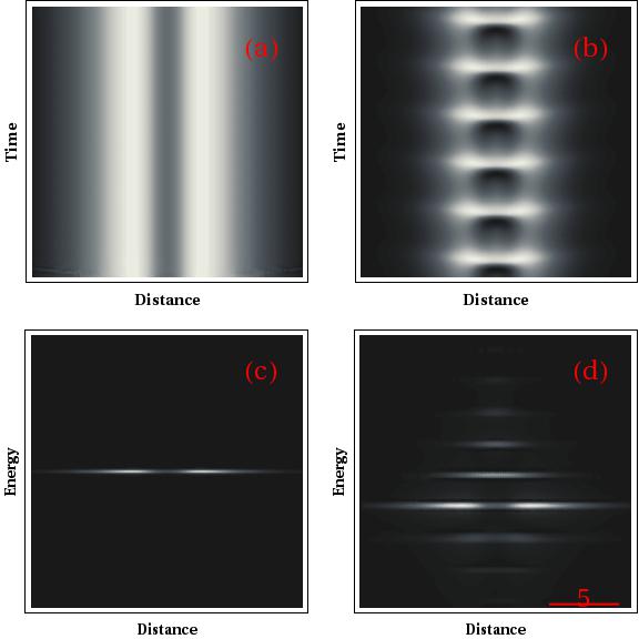
We compare two cases: the cGL equation by letting $\delta=0$ in Eq. (46) and the cSH equation with $\delta=0.1,\Delta_{e}=-1$. In the case of the evolution according to the cGL equation the system reaches the steady state, see Fig.1(a) which shows on the tomography image Fig 1(c) as a single energy level. The evolution according to the cSH equation leads to periodic oscillations of the density profile shown on Fig. 1(b). The corresponding tomography image on Fig. 1 shows several discrete energy levels. Similar behaviour has been observed in some experiments, eg. Roumpos:2010kta .

Figure 1: Comparison between solutions of the cGL and cSH equations for a single pumping spot. Time evolution of the density measured across the pumping spot (a) for the cGL equation and (b) cSH equation. Energy of the solutions across the pumping spot (c) for the cGL equation and (d) cSH equation. The results of the numerical simulations of Eq. (46) with the parameters given in (47).

0.3.3 Inhomogeneous energy (trapping)

We now turn to consider the behaviour in the presence of an harmonic trap Balili:2007gca ; Klaers:2010bi . We will consider how the presence of the dissipative terms in the general order parameter equation affects the stability of known solutions of the Gross Pitaevskii equation. We will look both at linear stability analysis (where one can gain insights from analytical results found by considering the perturbative effect of dissipation), as well as full numerical time evolution to find the new steady states.

As a starting point in the absence of dissipative terms, the Gross-Pitaevskii equation:

$$\partial_{t}\psi=i(\nabla^{2}-r^{2}-U_{0}|\psi|^{2})\psi$$ (48)

can be approximately solved by the stationary Thomas-Fermi profile with $\partial_{t}\psi=-i\mu\psi$ and $|\psi|^{2}=\Theta(\mu-r^{2})(\mu-r^{2})/U_{0}$. This density profile results from neglecting the kinetic energy. This is valid as long as the cloud size $r_{TF}=\sqrt{\mu}$ is large compared to the healing length $1/\sqrt{U_{0}}$, i.e. for $\sqrt{U_{0}\mu}\gg 1$. This stationary Thomas-Fermi profile gives a simple prescription for how to find the density profile in a given potential landscape. However, as will be discussed below, the stationary profile does not necessarily remain stable in the presence of the additional terms in Eq. (40).

Stability analysis

Starting from Eq. (40) with $\alpha,\beta,\delta,\eta=0$, we consider in turn the effects introduced by adding these dissipative terms. We restrict to considering $\Delta_{e}<0$ and neglect the superdiffusion term; after rescaling parameters, we may write:

$$2{\partial_{t}\psi}-i\left(\nabla^{2}-r^{2}-|\psi|^{2}\right)\psi=\left[\tilde{\alpha}-\tilde{\beta}|\psi|^{2}+\tilde{\delta}(2\tilde{\Delta}_{e}-\nabla^{2})\nabla^{2}-2i\tilde{\eta}{\partial_{t}}\right]\psi$$ (49)

in which all dissipative terms are placed on the right hand side. We then proceed by considering normal modes around the stationary solution in an approximation where the quantum pressure terms can be neglected, this is done by writing the equations in terms of density and phase and neglecting all quantum-pressure-like terms:

$$\partial_{t}\rho+\nabla\cdot(\rho\nabla\phi)=\left(\tilde{\alpha}-\tilde{\beta}\rho+2\tilde{\eta}\partial_{t}\phi-2\tilde{\delta}(\nabla\phi)^{2}\right)\rho,$$ (50)

$$2\partial_{t}\phi+(\nabla\phi)^{2}+r^{2}+\rho=\tilde{\delta}(2\tilde{\Delta}_{e}\nabla^{2}-\nabla^{4})\phi.$$ (51)

In the absence of the dissipative terms, this problem is the two-dimensional analog of that studied by Stringari Stringari1996 ; Stringari1998 . Linearising these equations using $\rho\to\rho+he^{-i\omega t},\phi\to\phi+\varphi e^{-i\omega t}$ yields normal modes with frequencies $\omega_{ns}=\sqrt{2n^{2}+2(s+1)n+s}$ and density profiles given by hypergeometric functions $h(r,\theta)\propto{}_{2}F_{1}(-n,n+s+1;s+1,r^{2})e^{is\theta}r^{s}$; here $n$ is a radial quantum number, and $s$ is an angular quantum number. Including dissipative terms, these normal mode frequencies acquire imaginary parts, describing either growth or decay of such fluctuations. Instability of the stationary state occurs when at least one of these fluctuation modes grows.

To account for dissipative terms perturbatively, it is enough to take the normal mode functions found in the absence of dissipation and find the first order frequency shift induced by the dissipative terms. At first order in the dissipative terms, there is no change to the density profile; however a non-zero phase gradient $\nabla\phi$ does appear at first order in the dissipative terms. Vanishing of the current at the edge of the cloud then requires $\mu=3\tilde{\alpha}/(2\tilde{\beta}+3\tilde{\eta})$.

Formally one may write the linearised form of Eq. (50) in the form $-i\omega_{s,n}\chi_{s,n}(r,\theta)=\left(\mathcal{L}^{(0)}+\mathcal{L}^{(1)}\right)\chi_{s,n}$ in which $\mathcal{L}$ is a matrix of differential operators acting on the fluctuation term $\chi=(h,\varphi)^{T}$. By identifying the dissipative terms as $\mathcal{L}^{(1)}$, standard first order perturbation theory then yields the first order correction: $\omega^{(1)}_{ns}=i\langle\chi_{ns}^{(0)},\mathcal{L}^{(1)}\chi_{ns}^{(0)}\rangle/\langle\chi_{ns}^{(0)},\chi_{ns}^{(0)}\rangle$ where angle brackets indicate the appropriate inner product. Following this procedure, one eventually finds

$$\omega^{(1)}_{ns}=\frac{i}{2N}\int 2\pi rdr\left[(h_{ns}^{(0)})^{2}\left(\tilde{\alpha}-\tilde{\eta}\mu-(2\tilde{\beta}+\tilde{\eta})\mu\right)+\tilde{\delta}h_{ns}^{(0)}\left(\tilde{\Delta}_{e}-\frac{1}{2}\nabla^{2}\right)\nabla^{2}h_{ns}^{(0)}\right]$$ (52)

where the normalisation $N=\int 2\pi rdrh_{ns}^{2}$ and integration is over the area of the Thomas-Fermi profile $r^{2}<\mu$. The hypergeometric form of the zero order functions $h^{(0)}_{ns}$ allows Eq. (52) to be evaluated analytically. The terms proportional to $\tilde{\delta}$ in fact vanishes, and the remaining term can be written (making use of the above value of $\mu$) as:

$$\omega^{(1)}_{ns}=\frac{i\tilde{\alpha}}{4\tilde{\beta}+6\tilde{\eta}}\left[(6\tilde{\beta}+3\tilde{\eta})\left(\frac{s^{2}+(\omega_{ns}^{(0)})^{2}}{s^{2}+2(\omega_{ns}^{(0)})^{2}}\right)-4\tilde{\beta}-3\tilde{\eta}\right].$$ (53)

Crucially, $(\omega_{ns}^{(0)})^{2}$ as given above grows only linearly with $s$. Thus, at large $s$ the ratio in parentheses tends to one, and so $\omega^{(1)}_{ns}\to{i\tilde{\beta}\tilde{\alpha}}/(2\tilde{\beta}+3\tilde{\eta})>0$ This positive value means that there is an instability, even for non-zero $\tilde{\eta}$. Although neither $\tilde{\eta}$ nor $\tilde{\delta}$ remove the instability in this perturbative approach, this does not prevent these terms from restoring stability via higher order corrections. This needs to be checked by numerical simulations.

Vortex lattices

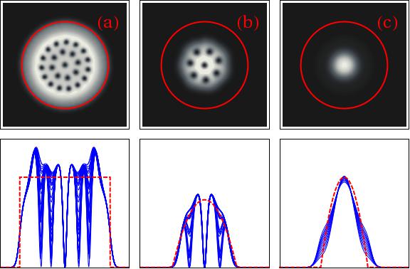
Having seen that the stationary profile possesses an instability, we next consider the behaviour resulting from this instability. In order to reach a final configuration, it is necessary to restrict the pumping to a finite range. We thus take and $\tilde{\alpha}({\bf r})=\tilde{\alpha}_{0}\theta(r_{0}-r)$, $\tilde{\alpha}_{0}=8$, $\tilde{\beta}=0.6$, where the pumping is a flat top of the radius $r_{0}=7$. For $\tilde{\eta}=\tilde{\delta}=0$, this model has been found to evolve to a rotating vortex latticeKeeling:2008hj . If one also includes the superdiffusion present in the cSH model, one finds that (in contrast to the linearised analysis) this may arrest the instability to vortex formation, and thus lead instead to an oscillating vortex-free state. Fig. 2 compares the profiles that result from the numerical simulation of Eq. (46) for the cases of the cGL equations for $\tilde{\eta}=0$ (Fig. 2(a)), $\tilde{\eta}=0.2$ (Fig. 2 (b)) and the cSH equation with $\tilde{\eta}=\tilde{\delta}=0.2$ and $\tilde{\Delta}_{e}=-0.5$ (Fig. 2 (c)).

Figure 2: Density plots of the polariton condensate in a harmonic trap according to the cGL equation with $\eta=0$ (a), $\eta=0.2$ (b) and the cSH equation with $\delta=\eta=0.2$ and $\Delta_{e}=-0.5$ (c). Top panels: luminosity is proportional to density. Red circles show the size of the pumping spot. Bottom panels: (solid lines) density of the cross section of the condensate at various times; (dashed lines) analytic approximations, given for (a) and (b) by Eq. (58), and for (c) by the Thomas-Fermi profile $\Theta(\mu-r^{2})(\mu-r^{2})$ with $\mu=3\tilde{\alpha}_{0}/(2\tilde{\beta}+3\tilde{\eta})$.

Although the presence of $\tilde{\eta}$ does not remove the instability, it does significantly effect the resulting rotating profile. This can both be seen in the numerical results shown in Fig. 2, and can also be understood by considering the $\tilde{\delta}=0$ limit of Eq. (50), written in a rotating frame. In a rotating frame, we consider solutions to Eq. (49) of the form:

$$2i\frac{\partial}{\partial t}\psi=\left(\mu-2i{\bf\Omega}\cdot\vec{r}\times\nabla\right)\psi$$ (54)

such that the time dependence has two parts: rotation with angular velocity ${\bf\Omega}=(0,0,\Omega)$, and phase accumulation at rate $\mu$. Inserting this ansätz into Eq. (49) and then making the Madellung transform, with neglect of quantum pressure terms, one finds:

$$\nabla\cdot\left[\rho(\nabla\phi-{\bf\Omega}\times\vec{r})\right]=\left[\tilde{\alpha}-\tilde{\beta}\rho-\tilde{\eta}\left(\mu+2{\bf\Omega}\times\vec{r}\cdot\nabla\phi\right)\right]\rho$$ (55)

$$-\mu+(\nabla\phi-{\bf\Omega}\times\vec{r})^{2}+(1-\Omega^{2})r^{2}+\rho=0$$ (56)

These equations can be satisfied by setting $\nabla\phi\simeq{\bf\Omega}\times\vec{r}$ which yields:

$$0=\tilde{\alpha}-\tilde{\beta}\rho-\tilde{\eta}\left(\mu+2\Omega^{2}r^{2}\right),\qquad-\mu+(1-\Omega^{2})r^{2}+\rho=0$$ (57)

These give two equations for $\rho$ which are both satisfied if:

$$\rho=\mu-(1-\Omega^{2})r^{2}=\frac{1}{\tilde{\beta}}\left[\tilde{\alpha}-\tilde{\eta}(\mu+2\Omega^{2}r^{2})\right]$$ (58)

hence $\Omega^{2}=\tilde{\beta}/(\tilde{\beta}+2\tilde{\eta}),\mu=\tilde{\alpha}/(\tilde{\beta}+\tilde{\eta})$. This indicates that while for $\tilde{\eta}=0$, the lattice rotates at $\Omega=1$, cancelling out the trapping potential, for finite $\eta$, the rotation velocity decreases, hence the density profile becomes non-flat, as seen in Fig. 2

In the above, $\nabla\phi\simeq{\bf\Omega}\times\vec{r}$ would require the phase profile to mimic solid body rotation. For a condensate, this cannot be exactly satisfied, but can be approximately satisfied (on a coarse grained scale) by having a density of vortices $\Omega$. Since increasing $\tilde{\eta}$ causes $\Omega$ to decrease, a sufficiently large value of $\tilde{\eta}$ can in effect kill any finite vortex lattice by reducing the vortex density to values so that the number of vortices falls below one.

0.4 Conclusions

We reviewed the connection between lasers, polariton condensates and equilibrium Bose condensates from a common framework based on order parameter equations. The cSH equations derived for lasers should be applicable to polariton condensates in the limit of non-negligible interactions and the stimulated scattering between polariton modes. The pattern formation in the framework of the cSH equations have been well-studied for lasers indicating a wealth of dynamics and phenomena. Some of these phenomena may be achieved in polariton condensates. At the same time the stronger nonlinearities and different external potentials (engineered or due to disorder) may lead to novel properties of the system exhibiting effects not seen in normal lasers.

References

- [1] A Amo, S Pigeon, D Sanvitto, V G Sala, R Hivet, I Carusotto, F Pisanello, G Lemenager, R Houdre, E Giacobino, C Ciuti, and A Bramati. Polariton Superfluids Reveal Quantum Hydrodynamic Solitons. Science, 332(6034):1167–1170, 2011.
- [2] Igor Aranson and Lorenz Kramer. The world of the complex Ginzburg-Landau equation. Rev. Mod. Phys., 74(1):99–143, 2002.
- [3] F Arecchi, G Giacomelli, P Ramazza, and S Residori. Vortices and defect statistics in two-dimensional optical chaos. Phys. Rev. Lett., 67(27):3749–3752, 1991.
- [4] R Balili, V Hartwell, D Snoke, L Pfeiffer, and K West. Bose-Einstein Condensation of Microcavity Polaritons in a Trap. Science, 316(5827):1007–1010, 2007.
- [5] A Buka, B Dressel, and L Kramer. Direct transition to electroconvection in a homeotropic nematic liquid crystal. Chaos, 14(3):793, 2004.
- [6] G Christmann, G Tosi, N G Berloff, P Tsotsis, P S Eldridge, Z Hatzopoulos, P G Savvidis, and J J Baumberg. Polariton ring condensates and sunflower ripples in an expanding quantum liquid. arXiv:1201.2113, 2012.
- [7] S M Cox, P C Matthews, and S L Pollicott. Swift-Hohenberg model for magnetoconvection. Phys. Rev. E, 69:066314, 2004.
- [8] M Cross and P Hohenberg. Pattern formation outside of equilibrium. Rev. Mod. Phys., 65(3):851–1112, 1993.
- [9] R Dodd, K Burnett, M Edwards, and C W Clark. Excitation spectroscopy of vortex states in dilute Bose-Einstein condensed gases. Phys. Rev. A, 56(1):587–590, 1997.
- [10] O Dzyapko, V E Demidov, and S O Demokritov. Ginzburg-Landau model of Bose-Einstein condensation of magnons. Phys. Rev. B, 81:024418, 2010.
- [11] S V Fedorov, A G Vladimirov, and G V Khodova. Effect of frequency detunings and finite relaxation rates on laser localized structures. Phys. Rev. E, 61:5814, 2000.
- [12] C Gardiner, P Zoller, R Ballagh, and M Davis. Kinetics of Bose-Einstein Condensation in a Trap. Phys. Rev. Lett., 79(10):1793–1796, 1997.
- [13] H E Hall and W F Vinen. The Rotation of Liquid Helium II. II. The Theory of Mutual Friction in Uniformly Rotating Helium II. Proc. Roy. Soc. A, 238(1213):215–234, 1956.
- [14] P Hohenberg and B Halperin. Theory of dynamic critical phenomena. Rev. Mod. Phys., 49(3):435–479, 1977.
- [15] A Imamoğlu and R J Ram. Quantum dynamics of exciton lasers. Phys. Lett. A, 214(3–4):193 – 198, 1996.
- [16] L P Kadanoff. Statistical Physics: Statics, Dynamics and Renormalization. World Scientific, Singapore, 2000.
- [17] J Kasprzak, M Richard, S Kundermann, A Baas, P Jeambrun, J M J Keeling, F M Marchetti, M H Szymańska, R André, J L Staehli, V Savona, P B Littlewood, B Deveaud, and Le Si Dang. Bose–Einstein condensation of exciton polaritons. Nature, 443(7110):409–414, 2006.
- [18] J Keeling and N G Berloff. Spontaneous Rotating Vortex Lattices in a Pumped Decaying Condensate. Phys. Rev. Lett., 100(25):250401, 2008.
- [19] J Klaers, J Schmitt, F Vewinger, and M Weitz. Bose–Einstein condensation of photons in an optical microcavity. Nature, 468(7323):545–548, 2010.
- [20] B Kneer, T Wong, K Vogel, W Schleich, and D Walls. Generic model of an atom laser. Phys. Rev. A, 58(6):4841–4853, 1998.
- [21] N Kopnin. Theory of Nonequilibrium Superconductivity. Oxford University Press, Oxford, 2001.
- [22] D Krizhanovskii, K Lagoudakis, M Wouters, B Pietka, R Bradley, K Guda, D Whittaker, M Skolnick, B Deveaud-Plédran, M Richard, R André, and Le Dang. Coexisting nonequilibrium condensates with long-range spatial coherence in semiconductor microcavities. Phys. Rev. B, 80(4):045317, 2009.
- [23] Y Kuramoto and T Tsuzuki. Persistent propagation of concentration waves in dissipative media far from thermal equilibrium. Prog. Theor. Phys., 55:356, 1976.
- [24] K G Lagoudakis, M Wouters, M Richard, A Baas, I Carusotto, R André, Le Si Dang, and B Deveaud-Plédran. Quantized vortices in an exciton–polariton condensate. Nature Physics, 4(9):706–710, 2008.
- [25] J Lega, J Moloney, and A Newell. Swift-Hohenberg Equation for Lasers. Phys. Rev. Lett., 73(22):2978–2981, 1994.
- [26] T Liew, A Kavokin, and I Shelykh. Excitation of vortices in semiconductor microcavities. Phys. Rev. B, 75(24):241301(R), 2007.
- [27] L A Lugiato, C Oldano, and L M Narducci. Cooperative frequency locking and stationary spatial structures in lasers. J. Opt. Soc. Am. B, 5(5):879–888, 1988.
- [28] P Manneville. Spots and turbulent domains in a model of transitional plane couette flow. Theoretical and Computational Fluid Dynamics, 18:169–181, 2004. 10.1007/s00162-004-0142-4.
- [29] B J Matkowsky and A A Nepomnyashchy. A complex Swift–Hohenberg equation coupled to the Goldstone mode in the nonlinear dynamics of flames. Physica D: Nonlinear Phenomena, 179(3-4):183, 2003.
- [30] J V Moloney and A C Newell. Universal description of laser dynamics near threshold. Physica D: Nonlinear Phenomena, 83(4):478–498, 1995.
- [31] A Penckwitt, R Ballagh, and C Gardiner. Nucleation, Growth, and Stabilization of Bose-Einstein Condensate Vortex Lattices. Phys. Rev. Lett., 89(26):260402, 2002.
- [32] L M Pismen. Vortices in Nonlinear Fields. From Liquid Crystals to Superfluids, From Non-Equilibrium Patterns to Cosmic Strings. Oxford University Press, Oxford, 1999.
- [33] G Roumpos, W H Nitsche, S Höfling, A Forchel, and Y Yamamoto. Gain-Induced Trapping of Microcavity Exciton Polariton Condensates. Phys. Rev. Lett., 104(12):126403, 2010.
- [34] G I Sivashinsky. Nonlinear analysis of hydrodynamic instability in laminar flames–i. derivation of basic equations. Acta Astronaut, 4:1177–1206, 1977.
- [35] K Staliunas. Laser Ginzburg-Landau equation and laser hydrodynamics. Phys. Rev. A, 48(2):1573–1581, 1993.
- [36] S Stringari. Collective Excitations of a Trapped Bose-Condensed Gas. Phys. Rev. Lett., 77(12):2360–2363, 1996.
- [37] S Stringari. Dynamics of Bose-Einstein condensed gases in highly deformed traps. Phys. Rev. A, 58(3):2385–2388, 1998.
- [38] V Taranenko, K Staliunas, and C Weiss. Spatial soliton laser: Localized structures in a laser with a saturable absorber in a self-imaging resonator. Phys. Rev. A, 56(2):1582–1591, 1997.
- [39] G Tosi, G Christmann, N G Berloff, P Tsotsis, T Gao, Z Hatzopoulos, P G Savvidis, and J J Baumberg. Sculpting oscillators with light within a nonlinear quantum fluid. Nature Physics, 8:190–194, 2012.
- [40] E Wertz, L Ferrier, D D Solnyshkov, P Senellart, D Bajoni, A Miard, A Lemaı̂tre, G Malpuech, and J Bloch. Spontaneous formation of a polariton condensate in a planar GaAs microcavity. Appl. Phys. Lett., 95(5):051108–051108–3, 2009.
- [41] M Wouters. Excitations and superfluidity in non-equilibrium Bose–Einstein condensates of exciton–polaritons. Superlattices and Microstructures, 43(5–6):524–527, 2008.
- [42] M Wouters and I Carusotto. Excitations in a Nonequilibrium Bose-Einstein Condensate of Exciton Polaritons. Phys. Rev. Lett., 99(14):140402, 2007.
- [43] M Wouters and I Carusotto. Superfluidity and Critical Velocities in Nonequilibrium Bose-Einstein Condensates. Phys. Rev. Lett., 105(2):020602, 2010.
- [44] M Wouters, T Liew, and V Savona. Energy relaxation in one-dimensional polariton condensates. Phys. Rev. B, 82(24):245315, 2010.