Vacuum fluctuations and generalized boundary conditions

Abstract

We present a study of the static and dynamical Casimir effects for a quantum field theory satisfying generalized Robin boundary condition, of a kind that arises naturally within the context of quantum circuits. Since those conditions may also be relevant to measurements of the dynamical Casimir effect, we evaluate their role in the concrete example of a real scalar field in $1+1$ dimensions, a system which has a well-known mechanical analogue involving a loaded string.

I Introduction

Over the course of the last 15 years, there has been a renewed interest in the Casimir effect. This was partly due to a second generation of experiments, started in 1997, which triggered a sustained flow of both theoretical and experimental works. As an outcome of those works, our knowledge about the dependence of Casimir forces on the geometry and material properties of the objects involved has remarkably improved libros .

The dynamical counterpart of the Casimir effect, also known as ‘motion induced radiation’, has also been the subject of intense research, manifested in the consequent profusion of works reviews dce . Although the direct measurement of radiation generated by moving mirrors is a daunting experimental challenge, photon creation induced by time dependent external boundary conditions has, indeed, been observed experimentally, albeit in a different context, namely, superconducting circuits wilson1 . There are also ongoing experiments aimed at measuring the photon creation induced by the time dependent conductivity of a semiconductor slab enclosed by an electromagnetic cavity padova , and proposals based on the use of high frequency resonators to produce the photons, and ultracold atoms to detect the created photons via superradiance Kim06 .

The superconducting circuit experiment mentioned above wilson1 , consists of a coplanar waveguide terminated by a SQUID, upon which a time dependent magnetic flux is applied. This system can be described by a quantum scalar field $\phi(x,t)$ (the magnetic flux at the different positions of the transmission line) satisfying on the SQUID (located at $x=a$) the boundary condition Johansson

$$\frac{1}{L}\frac{\partial\phi}{\partial x}(a,t)+C\frac{\partial^{2}\phi}{\partial t^{2}}(a,t)+E(t)\phi(a,t)=0\,,$$ (1)

where $C$ and $L$ are constants, and $E(t)$ is proportional to the (time-dependent) external magnetic flux. Equation (1) can be interpreted as a sort of generalized Robin boundary condition, because of the presence of the term with second-order time derivatives. The theoretical analysis of that experiment was done assuming that the term proportional to the second derivative of the field is negligible Johansson . Whence the boundary condition became a standard Robin boundary condition with a time dependent, externally driven parameter. The boundary condition that results after implementing this approximation, has been described in terms of an effective length wilson1 ; Johansson .

From a theoretical point of view, the particle creation rate for the case of a quantum field satisfying (time independent) Robin boundary conditions on a moving mirror has been investigated in Ref. farina2006 . The complementary situation, namely, time dependent Robin boundary conditions on a static mirror have been considered in Refs. farina2011 ; farina2012 . It is the aim of this work to consider the static and dynamical Casimir effects for quantum fields which are subject to generalized boundary conditions of the type defined in Eq.(1). Our interest in this problem is twofold. On the one hand, the presence of the second derivative of the field in the boundary condition modifies the usual Sturm-Liouville problem, what manifests itself in the existence of an eigenvalue-dependent boundary condition. This problem, well-known to mathematicians, has also been considered in different areas of physics. It has not, however, to our knowledge, been dealt with in the Casimir effect context.

Regarding the experimental relevance of the inclusion of this kind of term, we note that, although it may be neglected in the particular experimental setup considered in Ref. wilson1 , this contribution to the boundary condition may indeed affect the spectral distribution of the created particles farina2012 , something to which future experiments might be sensitive.

This paper is organized as follows. In Section II, we describe the classical aspects of the model, including a mechanical analogue, a discussion of the eigenvalue problem and the necessity of modifying the inner product between eigenfunctions due to the presence of the second order derivative in the boundary condition. In Section III we compute the static vacuum energy, Section IV deals with the dynamical Casimir effect, and Section V contains our conclusions.

II Classical model: the loaded string analogy

II.1 A mechanical analogue

Many different boundary conditions a scalar field in $1+1$ dimensions can be subject to, can be realized in classical mechanics analogues, based on vibrating strings. Indeed, Dirichlet boundary conditions correspond to a string with fixed endpoints, while Neumann conditions can be implemented by attaching, to the corresponding endpoint, a massless ring which can slide freely and frictionless along a vertical rod. Robin boundary conditions result, in turn, when the ring is also coupled to a vertical spring farina2012 . Finally, the generalized boundary condition of Eq.(1) can be generated by letting the ring be massive rather than massless (in all cases we will consider the linear regime, i.e. small amplitude oscillations of the string).

To see this, let us assume $T$ to be the string tension, $\mu$ its mass density, and that its configuration may be described by a single function $y(x,t)$, measuring its vertical departure from the equilibrium configuration. Denoting by $m$ the mass of the ring and by $\kappa$ the spring constant, the position of the ring, $y(a,t)$ satisfies Newton’s equation:

$$m\ddot{y}(a,t)=-\kappa y(a,t)-Ty^{\prime}(a,t)\;,$$ (2)

which has the same form as the generalized boundary condition of Eq.(1). The vibrating string problem with this kind of condition on one of its endpoints constitutes a well known problem in classical vibrations.

We stress that the boundary condition for the deformation of the string is in fact the dynamical equation for the position of the ring $q(t)\equiv y(a,t)$, and this is the origin of the presence of second order time derivatives in the generalized boundary condition. A proper treatment of the system should regard $q(t)$ and $y(x,t)$ as qualitatively different degrees of freedom, in the sense that $q$ has a discrete, finite mass, while $y$ is endowed with a continuous mass density. An enlightening way to treat this kind of problem can be seen, for example, in Jaroszkiewicz:1989zs , where the quantization of a non relativistic string with an arbitrary mass distribution has been considered. There, a system with a single continuous mass distribution which approximates the mixed continuous and discrete case has been considered. In this way, all the steps of the Lagrangian and Hamiltonian formalisms, and even canonical quantization, are well defined. The desired mass distribution is approached at the end of the process, as a special limit, after all the stumbling blocks in the procedure are avoided.

We will follow here an alternative procedure, which, as we have explicitly checked, yields the same results. Since the difficulties in the problem at hand come from the fact that the discrete mass is precisely at one of the endpoints of the system, we avoid the coincidence of those two singularities by temporarily splitting them. Indeed, we shall first assume that the mass $m$ is located at an arbitrary position $x_{0}$, $0<x_{0}<a$, and impose Neumann boundary conditions at $x=0$ and $x=a$. The generalized Robin boundary condition at $x=a$ is then recovered by taking the ‘coincidence limit’ $x_{0}\to a^{-}$.

The classical Lagrangian then reads:

$$L = \frac{1}{2}\int_{0}^{a}dx\,\left[\mu\left(\frac{\partial y}{\partial t}\right)^{2}-T\left(\frac{\partial y}{\partial x}\right)^{2}\right.$$ (3)

$$\left.-\kappa y^{2}\delta(x-x_{0})+m\left(\frac{\partial y}{\partial t}\right)^{2}\delta(x-x_{0})\right]\;,$$

with Neumann conditions implicitly assumed at $x=0$ and $x=a$.

From the classical equation of motion one can easily check that the presence of a localized mass on the string induces a discontinuity in the spatial derivative of $y$,

$$T\left(\frac{\partial y}{\partial x}|_{x_{0}^{+}}-\frac{\partial y}{\partial x}|_{x_{0}^{-}}\right)=m\ddot{y}(x_{0},t)+\kappa y(x_{0},t)\,.$$ (4)

Note that the string can interchange energy with the mass, and the conserved total energy of this system reads

$$E = \frac{1}{2}\int_{0}^{a}dx\,\left[\mu\left(\frac{\partial y}{\partial t}\right)^{2}+T\left(\frac{\partial y}{\partial x}\right)^{2}\right]$$ (5)

$$+\frac{1}{2}\kappa y^{2}(x_{0},t)+\frac{1}{2}m\left(\frac{\partial y}{\partial t}\right)_{x=x_{0}}^{2}\;,$$

that is, the sum of the mechanical energies associated to the string and the ring.

II.2 A one dimensional cavity with localized conductivity and permittivity

Let us now focus on the analogous case of a scalar field in $1+1$ dimensions, as a toy model for the electromagnetic field in $3+1$ dimensions. We assume the Lagrangian to be given by the expression:

$$L = \frac{1}{2}\int_{0}^{a}dx\,\left[\epsilon(x,t)\left(\frac{\partial\phi}{\partial t}\right)^{2}-\left(\frac{\partial\phi}{\partial x}\right)^{2}\right.$$ (6)

$$\left.-V(x,t)\phi^{2}\right]\,,$$

with

$$\epsilon(x,t)=1+\chi(t)\delta(x-x_{0})\,,$$ (7)

and

$$V(x,t)=v(t)\delta(x-x_{0})\,.$$ (8)

As in the mechanical model, we shall regard this as a simple model to describe a cavity in which the permittivity and conductivity are concentrated at the point $x=x_{0}$, which, tending to $a$ from the left, reproduces the generalized Robin condition at $x=a$. The particular case $\chi(t)=0$ and $v(t)=v_{0}(1+f(t))$ has been considered in Ref.crocce , as a simple model of the experimental setup of Ref.padova (the generalization to the electromagnetic case has been analyzed in Ref.japon ). In Section III we will compute the Casimir interaction energy between two slabs described by constant values of $v=v_{0}$ and $\chi=\chi_{0}$. In Section IV we will compute the photon creation associated to a time dependent $v(t)$ and $\chi=\chi_{0}$.

II.3 Eigenfunctions and inner product

Let us consider the model given in Eq.(6), with Neumann boundary conditions at $x=0,a$. We will compute the eigenfunctions and eigenvalues for the particular case $v(t)=v_{0}$ and $\epsilon(t)=\chi_{0}$. The eigenmodes can be written as

$$\Psi_{k}(x,t)=N_{k}e^{-ikt}\left[\cos(kx)\cos(k(x_{0}-a))\theta(x_{0}-x)\right.$$

$$\left.+\cos(kx_{0})\cos(k(x-a))\theta(x-x_{0})\right]\equiv e^{-ikt}\psi_{k}(x)\,,$$ (9)

where $N_{k}$ is a normalization constant. They are continuous at $x=x_{0}$ and satisfy Neumann boundary conditions at $x=0,a$. The discontinuity equation at $x=x_{0}$ implies

$$k\sin(ka)=(v_{0}-\chi_{0}k^{2})\cos(kx_{0})\cos(k(x_{0}-a))\,,$$ (10)

which is the equation that defines the eigenfrequencies. In the particular case $x_{0}\to a$, the transcendental equation that defines the eigenfrequencies simplifies to

$$k\tan(ka)=(v_{0}-\chi_{0}k^{2})\,.$$ (11)

It is straightforward to show that, unless $\chi_{0}=0$, eigenfunctions corresponding to different eigenvalues are not orthogonal with the usual inner product. However, defining a generalized inner product (see the Appendix and Refs. Jaroszkiewicz:1989zs ; darma )

$$(\psi_{k},\psi_{k^{\prime}}) = \int_{0}^{a}dx\,\psi_{k}(x)\psi_{k^{\prime}}(x)+\chi_{0}\psi_{k}(a)\psi_{k^{\prime}}(a)$$ (12)

$$= \int_{0}^{a}dx\,\epsilon(x)\psi_{k}(x)\psi_{k^{\prime}}(x)$$

one can check the orthogonality $(\psi_{k},\psi_{k^{\prime}})=0$ for $k\neq k^{\prime}$. With appropriate normalization, the eigenfunctions can be chosen to be orthonormal, as we shall assume it has been done in what follows.

This phenomenon is a general feature of the hybrid continuous plus discrete systems, where one can show that the eigenfunctions of the Hamiltonian are orthogonal for a scalar product defined in terms of a kernel Jaroszkiewicz:1989zs , which defines a Sturm-Liouville problem.

The equations above are valid even in the time-dependent case $v_{0}\to v(t)$, in which the eigenvalues become parametrically dependent on time, as well as the eigenfunctions $\psi_{k}$. We will analyze the time-dependent situation in Section IV.

Writing the field $\phi$ as a linear combination of the spatial eigenfunctions

$$\phi(x,t)=\sum_{k}Q_{k}(t)\psi_{k}(x)\,,$$ (13)

and inserting this expression into the classical Lagrangian one can check that it reduces to a set of uncoupled harmonic oscillators $Q_{k}$, with frequency $k$:

$$L=\frac{1}{2}\sum_{k}(\dot{Q}_{k}^{2}-k^{2}Q_{k}^{2})\;.$$ (14)

Details of this calculation are presented in the Appendix. Note that the additional term in the inner product Eq.(12) is crucial to cancel the kinetic term concentrated at $x_{0}$. Note also that these results can be straightforwardly generalized to cases where several slabs are located at different positions.

III Static Casimir effect

Once the system has been reduced to a set of uncoupled harmonic oscillators, the calculation of the vacuum energy can be performed by direct mode-summation. We will explicitly compute the static Casimir effect for two different physical situations: the interaction between two thin slabs, each one described by its conductivity and permittivity (in free space), and a system that satisfies generalized boundary conditions.

III.1 Interaction vacuum energy for two slabs

Let us consider two slabs, located at $x=\pm a/2$, and described by permittivities $\chi_{0}^{\pm}$ and conductivites $v^{\pm}$, respectively. In order to have a discrete set of eigenfrequencies, we enclose the system in a box of size $2L$, and impose Neumann boundary conditions at $x=\pm L$. As we will take the limit $L\gg a$ at the end of the calculation, the result will be independent of $L$ and of the boundary condition imposed at $x=\pm L$.

The eigenfunctions that satisfy Neumann boundary conditions at $x=\pm L$ can be written as

$$f_{\omega}(x)=\left\{\begin{array}[]{cl}A_{1}\cos[\omega(x+L)]&{\rm for}\,-L<x<-\frac{a}{2}\\ A_{2}\cos(\omega x)+A_{3}\sin(\omega x)&{\rm for}\,-\frac{a}{2}<x<\frac{a}{2}\\ A_{4}\cos[\omega(x-L)]&{\rm for}\,\frac{a}{2}<x<L\,.\end{array}\right.$$ (15)

The function $f_{\omega}(x)$ must be continuous at $x=\pm a/2$ and the spatial derivatives must satisfy:

$${\rm disc}[\partial_{x}f_{\omega}]_{x=\pm a/2}=[v_{0}^{\pm}-\chi_{0}^{\pm}\omega^{2}]f_{\omega}(\pm\frac{a}{2})\,.$$ (16)

The eigenfrequencies are the solutions of $\det M=0$, where $M(a,L,\omega)$ is the $4\times 4$ matrix associated to the linear system of equations for the coefficients $A_{i}$ derived by inserting Eq.(15) in Eq.(16). After some straightforward calculations one can show that

$$\det[M(a,L,\omega)]=\Delta^{+}\Delta^{-}(\sin(2\omega(a-L))+2\sin(a\omega))+$$

$$2(\Delta^{+}+\Delta^{-})\cos(a\omega)+(\Delta^{+}\Delta^{-}-4)\sin(2L\omega)+$$

$$2(\Delta^{+}+\Delta^{-})\cos(2L\omega)\,\,,$$ (17)

where $\Delta^{\pm}=\frac{1}{\omega}(v_{0}^{\pm}-\chi_{0}^{\pm}\omega^{2})$.

We will compute the Casimir energy as the difference between the zero point energy of the slabs separated by a distance $a$, and that corresponding to a distance $l\gg a$. Using the argument theorem, we see that:

$$E_{C}(a) = \frac{1}{2}\sum_{n}(\omega_{n}-\tilde{\omega}_{n})$$ (18)

$$= -\frac{1}{4\pi i}\oint dz\,\log\det\left[\frac{M(a,L,z)}{M(l,L,z)}\right]\,,$$

where $\omega_{n}$ and $\tilde{\omega}_{n}$ are the eigenfrequencies associated to the distances $a$ and $l$, respectively. The integration path must include the real positive axis. Following standard steps, and taking the limit $L\to\infty$, we arrive to an integral in the imaginary-frequency axis $z=i\xi$:

$$E_{C}=\frac{1}{2\pi}\int_{0}^{\infty}d\xi\,\log\big{[}1-e^{-2\xi a}C(\xi)\big{]}\;,$$ (19)

where

$$C(\xi)=\frac{(v_{0}^{+}+\chi_{0}^{+}\xi^{2})(v_{0}^{-}+\chi_{0}^{-}\xi^{2})}{(2\xi+v_{0}^{+}+\chi_{0}^{+}\xi^{2})(2\xi+v_{0}^{-}+\chi_{0}^{-}\xi^{2})}\,.$$ (20)

Not surprisingly, for the particular case $\chi_{0}^{\pm}=0$, this result coincides with the usual Casimir energy for the so called $\delta$-potentials. Moreover, in the $v_{0}^{\pm}\to\infty$ limit, one has $C(\xi)\to 1$, and the result reproduces the usual one for Dirichlet boundary conditions. Note that, as $\partial C/\partial\chi_{0}^{\pm}>0$, the presence of the second order time derivative in the boundary conditions enhances the interaction between slabs.

It is interesting to remark that the final result for the Casimir energy is tantamount to the one corresponding to a $\delta$-potential with a frequency-dependent coefficient $v(\omega)=v_{0}-\chi_{0}\omega^{2}$. Therefore, this result could have been derived using Lifshitz formula with the particular reflection coefficients that describe the slabs. The above calculation is an alternative and equivalent way to compute the vacuum energy, that shows that the Casimir energy is just the sum over the eigenfrequencies defined by the $\omega$-dependent boundary conditions.

III.2 Interaction vacuum energy for generalized boundary conditions

We now consider the second case, namely, a system that satisfies Neumann boundary conditions at $x=0$ and generalized Robin boundary conditions at $x=a$. The eigenfrequencies are defined implicitly by Eq.(11), that we rewrite as $G(a,\omega)=0$, with

$$G(a,\omega)=\omega\sin(\omega a)-(v_{0}-\chi_{0}\omega^{2})\cos(\omega a)\,.$$ (21)

As in the previous subsection, we enclose the system in a large box of size $2L$, and impose Neumann boundary conditions at $x=\pm L$. The eigenfrequencies are thus determined by the equation $\tilde{G}(a,L,\omega)=0$, with

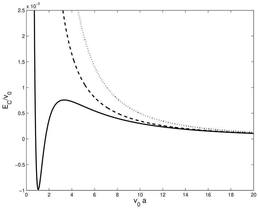
Figure 1: Dimensionless total Casimir energy $E_{C}/v_{0}$ as a function of the distance $v_{0}a$, for different values of $v_{0}\chi_{0}$. While the force is always repulsive for large values of $v_{0}\chi_{0}$, for $v_{0}\chi_{0}=0.1$ (solid line) it starts being repulsive, then becomes attractive, and is finally repulsive again for larger values of the distance. Dashed line corresponds to $v_{0}\chi_{0}=0.5$, and the dotted line corresponds to $v_{0}\chi_{0}=5$

$$\tilde{G}(a,L,\omega)=G(a,\omega)\sin[\omega(L-a/2)]^{2}\,.$$ (22)

Then we compute the Casimir energy as the difference between the vacuum energy associated to the length $a$, and that associated to $l$ with $l\gg a$. Using again the argument theorem

$$E_{C}(a)=-\frac{1}{4\pi i}\oint dz\,\log\left[\frac{\tilde{G}(a,L,z)}{\tilde{G}(l,L,z)}\right]\,.$$ (23)

the final result can be written as

$$E_{C}=\frac{1}{2\pi}\int_{0}^{\infty}d\xi\,\log(1-e^{-2\xi a}B(\xi))\,,$$ (24)

where the function $B$ contains the information about the generalized boundary condition

$$B(\xi)=\frac{\xi-v_{0}-\chi_{0}\xi^{2}}{\xi+v_{0}+\chi_{0}\xi^{2}}\,.$$ (25)

As the sign of $B$ depend on the values of $v_{0}$, $\chi_{0}$ and $\xi$, the force can be attractive or repulsive depending on the value of $a$.

In oder to analyze the behavior of the energy with the different parameters, it is useful to note that

$$\frac{E_{C}}{v_{0}}=h(v_{0}a,v_{0}\chi_{0})\,,$$ (26)

where $h$ is a dimensionless function. This can be easily checked changing variables $\xi\to\xi/v_{0}$ in Eq.(24). Therefore, the qualitative dependence of the energy with the distance only depends on the dimensionless quantity $v_{0}\chi_{0}$. For instance, when $v_{0}\chi_{0}>1/4$, $B$ is negative for all values of $\xi$, and therefore the force is repulsive. In particular, in the limit $v_{0}\to\infty$, the boundary condition at $x=a$ becomes Dirichlet boundary condition, and one has $B\to-1$. The Casimir energy becomes the standard result for a scalar field satisfying Neumann boundary conditions at $x=0$ and Dirichlet boundary conditions at $x=a$, which corresponds to a repulsive force. When $v_{0}\chi_{0}<1/4$, we cannot predict the sign of the force analytically.

In Fig. 1 we present some numerical evaluations of Eq.(24). We refer all the ingredients in the expression for the energy to the dimensionful quantity, $v_{0}$. We plot the Casimir dimensionless energy $E_{C}/v_{0}$ as a function of the distance $a$ (in units of $v_{0}$) for different values of $v_{0}\chi_{0}$. We see that for small distances, the force changes sign for the smaller value of $v_{0}\chi_{0}=0.1$. In this regime, the force cross from repulsive to attractive and back sign to repulsive again, as the distance increases. For other values of $v_{0}\chi_{0}>1/4$ the force is, as expected, always repulsive.

IV Dynamical Casimir effect

Let us now consider the case of a time dependent $v(t)=v_{0}(1+f(t))$ and constant $\chi(t)=\chi_{0}$. In order to analyze this problem one can proceed as usual reviews dce ; crocce ; trembling , showing that, at the classical level, the system can be described by a set of coupled harmonic oscillators with time dependent frequencies and couplings. To this end, we introduce an ‘instantaneous basis’ $\psi_{k}(x,t)$ through the equations

$$\psi_{k}^{\prime\prime}+k^{2}(t)\psi_{k} = 0$$

$$\psi_{k}^{\prime}(0) = 0$$

$$\psi_{k}^{\prime}(a) = 0$$

$$\psi_{k}^{\prime}(x_{0}^{+})-\psi_{k}^{\prime}(x_{0}^{-}) = (-\chi_{0}k^{2}+v(t))\psi_{k}\,.$$ (27)

Note that, due to the time dependent boundary condition at $x_{0}$, the eigenvalues are time dependent, and this induces a parametric time dependence in the basis functions. The limit $x_{0}\to a^{-}$ describes a cavity with a SQUID at one end, but one could consider more general situations like a cavity ended by two SQUIDs, or even a set of SQUIDs located at different positions in a waveguide.

We now expand the field using the instantaneous basis

$$\phi(x,t)=\sum_{k}Q_{k}(t)\psi_{k}(x,t)\,.$$ (28)

The classical Lagrangian given in Eq.(6) can be written in terms of the variables $Q_{k}$, as in the static case. The frequencies of the classical oscillators become time-dependent, and the Lagrangian contains additional terms proportional to derivatives of the basis functions, which in turn are proportional to the derivatives of the eigenvalues $\dot{k}(t)$.

As shown in the Appendix, the classical Lagrangian reads

$$L = \frac{1}{2}\sum_{k}(\dot{Q}_{k}^{2}-k^{2}(t)Q_{k}^{2})+\sum_{kj}A_{kj}(t)\dot{Q}_{k}Q_{j}$$ (29)

$$- \frac{1}{2}\sum_{kj}S_{kj}(t)Q_{k}Q_{j}\,,$$

where the time-dependent matrices $A_{kj}$ and $S_{kj}$ can be chosen to be antisymmetric and symmetric, respectively. The explicit expressions for them are derived in the Appendix. Note that, if the time dependence of the eigenvalues is proportional to a dimensionless parameter $\delta$, $A_{kj}=O(\delta)$ and $S_{kj}=O(\delta^{2})$ (see Eq.(51)).

Let us now assume that the externally driven property $v(t)$ has a harmonic time dependence with frequency $\Omega$. When the external frequency is tuned with an eigenfrequency of the static cavity $\Omega=2\tilde{k}_{0}$, with $\tilde{k}_{0}$ one of the solutions to Eq.(10), we expect the number of created photons to be enhanced by parametric resonance. Moreover, since in general the spectrum of the cavity is not regularly-spaced, it is reasonable to neglect couplings between modes detuning . The dynamics of the system is essentially given by that of the mode associated to $k_{0}$, i.e. a single harmonic oscillator with time dependent frequency:

$$L\simeq\frac{1}{2}[\dot{Q}_{k_{0}}^{2}-k_{0}^{2}(t)Q_{k_{0}}^{2}]\,,$$ (30)

where we have neglected terms of order $O(\delta^{2})$. Here $k_{0}(t)$ is a solution to

$$k\sin(ka)=(v(t)-\chi_{0}k^{2})\cos(kx_{0})\cos(k(x_{0}-a))\,.$$ (31)

For the sake of simplicity, we will solve this equation for $x_{0}\to a^{-}$. We denote by $\tilde{k}_{0}$ a solution to Eq.(31) in the static case $f(t)=0$. Assuming that $k_{0}(t)=\tilde{k}_{0}(1+\eta f(t))$, with $\eta f(t)\ll 1$, one can show that

$$\eta=\frac{v_{0}}{v_{0}+\tilde{k}_{0}^{2}(a+\chi_{0})+a(v_{0}-\chi_{0}\tilde{k}_{0}^{2})^{2}}\,.$$ (32)

When $f(t)=A\sin[2\tilde{k}_{0}t]$, the number of photons with frequency $\tilde{k}_{0}$ will grow exponentially. The calculation is, by now, standard reviews dce ; crocce ; trembling ; detuning , and will not be reproduced here. The result is

$$N_{\tilde{k}_{0}}(t)=\exp[{\tilde{k}}_{0}A\eta t]\equiv\exp[\lambda t]\,.$$ (33)

Note above equations are valid for small values of the aforementioned parameter $\delta=A\eta\ll 1$.

It is interesting to analyze two opposite limiting cases. When $v_{0}a\gg 1$, the lowest frequency solution is $\tilde{k}_{0}\simeq\pi/(2a)$, and therefore $\eta\simeq 1/(v_{0}a)$. The particle creation rate, in this case, is $\lambda=\pi A/(2v_{0}a^{2})$.

On the other hand, when $v_{0}a\ll 1$, the first solution to the transcendental Eq. (11) is

$$\tilde{k}_{0}a\simeq\sqrt{\frac{v_{0}a}{1+\frac{\chi_{0}}{a}}}\,.$$ (34)

In this case we have $\eta\approx 1/2$ (assuming that $\chi_{0}/a\ll 1$). Therefore, the corresponding rate is $\lambda=A/2\sqrt{v_{0}/a}$.

The last case may be of some interest for the experimental observation of the dynamical Casimir effect, since the Robin or generalized Robin boundary conditions may be adjusted in such a way to reduce the value of the lowest eigenfrequency of the unperturbed cavity. This point deserves further analysis.

When considering the parametric resonance situation, it is crucial to tune the external frequency with one of the eigenfrequencies of the system. The term proportional to $\chi_{0}$ in the boundary condition, however small, does introduce significant modifications to the static eigenfrequencies of the cavity. This effect may be relevant, for instance, for an experiment with a coplanar waveguide of finite size.

As an illustration of the last point, let us assume that $x_{0}\to a^{-}$ and that the external frequency is twice the lowest eigenfrequency of the cavity (that is, twice the first solution to Eq.(11)). In a realistic situation wustmann , $v_{0}a\gg 1$, and an approximate solution is $\tilde{k}_{0}\simeq\pi/(2a)$. Expanding the transcendental equation around this solution we obtain

$${\tilde{k}}_{0}\simeq\frac{\pi}{2a}(1-\frac{1}{v_{0}a}+\frac{1}{v_{0}^{2}a^{2}}-\frac{\pi^{2}}{4}\frac{\chi_{0}}{v_{0}^{2}a^{3}})\,.$$ (35)

Assuming wustmann $v_{0}a=20$ and $\chi_{0}/a=0.05$ the correction to the lowest eigenfrequency due to $\chi_{0}$ is $3\times 10^{-4}$. This small correction should be taken into account in order to achieve parametric resonance if the amplitude of the time-dependent external conditions is sufficiently small detuning .

V Conclusions

The original aim of this work has been to analyze the static and dynamical Casimir effects when the field satisfies generalized boundary conditions involving second order time derivatives. These conditions were in turn motivated by the effective boundary condition satisfied by the magnetic flux in a waveguide terminated by a SQUID, a setup that has been recently employed as a device to measure the creation of photons from the vacuum in the presence of time-dependent external fields wilson1 .

We have shown that this problem does have a simple and well-known classical analogue: a loaded string. From this point of view, the presence of the second-order time derivative is not surprising, since the boundary condition is in this case nothing but the dynamical equation for a massive ring attached to the end of the string. From a mathematical point of view, we have eigenvalue-dependent boundary conditions, and therefore the eigenfunctions associated to different eigenvalues are not orthogonal under the usual inner product. A generalization of the inner product makes them orthogonal. When expanding the deformation of the string in terms of spatial eigenfunctions, the additional term in the inner product exactly cancels out the kinetic term associated to the ring, and one ends up with a set of decoupled harmonic oscillators.

This mechanical analogy lead us to consider a more general situation, in which the ring is not attached to the end of the string; rather, it is located at an arbitrary distance from the endpoint. From a field-theory perspective, this can be considered as a toy model for an electromagnetic cavity in which one inserts a thin slab characterized by its conductivity and permittivity. From the quantum circuits point of view, this corresponds to a situation in which a SQUID is inserted in a one-dimensional waveguide.

Therefore, we computed the static Casimir interaction energy between two slabs, generalizing previous results for $\delta$-potentials. We also computed the static vacuum energy for the particular case in which the slab is near a border of the cavity. In summary, we have shown that the Casimir energy can be computed as the sum over modes satisfying the generalized Robin boundary condition.

Finally, and coming back to the original motivation, we considered some particular aspects of the dynamical Casimir effect for the generalized boundary conditions. On the one hand, we computed the particle creation rate assuming parametric resonance for the case of a finite waveguide ended by a SQUID. On the other hand, we discussed the influence of the second order time derivative on the tuning of the external pumping with one of the eigenfrequencies of the cavity. We have seen that the term proportional to $\ddot{\phi}$ in the boundary condition may indeed be relevant for this tuning.

The analysis of loaded strings with masses distributed periodically along it, or analogue acoustic and elastic systems, induces the presence of (approximate) band gaps in the spectrum bands . It would be interesting to analyze theoretically electromagnetic analogues of these configurations, like a waveguide with several SQUIDs, distributed periodically on it, or a microwave cavity with several slabs inserted accordingly.

Appendix A

In this Appendix we present some details of the calculations of the classical Lagrangian in both the static and dynamical cases.

To begin with, let us show that it is necessary to modify the usual inner product in order to have an orthonormal basis. The eigenfunctions satisfy

$$\psi_{k}^{\prime\prime}+k^{2}\psi_{k}=0$$ (36)

with the boundary conditions

$$\psi_{k}^{\prime}(0) = 0$$

$$\psi_{k}^{\prime}(a) = 0$$

$$\psi_{k}^{\prime}(x_{0}^{+})-\psi_{k}^{\prime}(x_{0}^{-}) = (-\chi_{0}k^{2}+v_{0})\psi_{k}\,.$$ (37)

For the sake of definiteness, we choose Neumann boundary conditions at $x=0,a$. The results below can be generalized to the case of Robin boundary conditions.

We compute

$$I_{ij}=\int_{0}^{a}(\psi_{i}^{\prime\prime}\psi_{j}-\psi_{i}\psi_{j}^{\prime\prime})dx=(j^{2}-i^{2})\int_{0}^{a}\psi_{i}\psi_{j}dx\,,$$ (38)

where in the last equality we used the eigenvalue equation. On the other hand we have

$$I_{ij}=\int_{0}^{a}[(\psi_{i}^{\prime}\psi_{j})^{\prime}-(\psi_{i}\psi_{j}^{\prime})^{\prime})dx=\chi_{0}(i^{2}-j^{2})\psi_{i}(x_{0})\psi_{j}(x_{0})\,.$$ (39)

One should be careful with the evaluation of

$$\int_{0}^{a}(\psi_{i}\psi_{j}^{\prime})^{\prime}dx$$ (40)

because of the discontinuity at $x_{0}$. Eq.(39) can be obtained writing $\int_{0}^{a}=\int_{0}^{x_{0}^{-}}+\int_{x_{0}^{+}}^{a}$ and using the boundary condition at $x_{0}$:

$$\int_{0}^{a}(\psi_{k}\psi_{j}^{\prime})^{\prime}dx = \psi_{k}(x_{0})[\psi_{j}^{\prime}(x_{0}^{-})-\psi_{j}^{\prime}(x_{0}^{+})]$$ (41)

$$= (\chi_{0}j^{2}-v_{0})\psi_{k}(x_{0})\psi_{j}(x_{0})$$

Subtracting Eqs.(38) and (39) we get

$$0=(j^{2}-i^{2})\left[\chi_{0}\psi_{i}(x_{0})\psi_{j}(x_{0})+\int_{0}^{a}dx\psi_{i}\psi_{j}\right]\,,$$ (42)

and therefore the inner product defined as

$$(\phi_{i},\phi_{j}) = \chi_{0}\psi_{i}(x_{0})\psi_{j}(x_{0})+\int_{0}^{a}dx\,\psi_{i}\psi_{j}$$ (43)

$$= \int_{0}^{a}dx\,\epsilon(x)\psi_{i}\psi_{j}\$$

vanishes when $i\neq j$.

To compute the static classical Lagrangian we write

$$\phi(x,t)=\sum_{k}Q_{k}(t)\psi_{k}(x)\,.$$ (44)

Therefore

$$\int_{0}^{a}dx\,\dot{\phi}^{2} = \sum_{kj}\dot{Q}_{k}\dot{Q}_{j}\int_{0}^{a}dx\,\psi_{k}\psi_{j}$$ (45)

$$= \sum_{kj}\dot{Q}_{k}\dot{Q}_{j}(\delta_{kj}-\chi_{0}\psi_{k}(x_{0})\psi_{j}(x_{0}))$$

$$= \sum_{k}\dot{Q}_{k}^{2}-\chi_{0}\dot{\phi}^{2}(x_{0})$$

A similar calculation can be done for the spatial derivatives

$$\int_{0}^{a}dx\phi^{\prime 2} = \sum_{kj}Q_{k}Q_{j}\int_{0}^{a}dx\psi_{k}^{\prime}\psi_{j}^{\prime}$$ (46)

$$= \sum_{kj}Q_{k}Q_{j}\int_{0}^{a}[(\psi_{k}\psi_{j}^{\prime})^{\prime}-\psi_{k}\psi_{j}^{\prime\prime})]$$

$$= \sum_{kj}Q_{k}Q_{j}\int_{0}^{a}[(\psi_{k}\psi_{j}^{\prime})^{\prime}+j^{2}\psi_{k}\psi_{j})]$$

Inserting Eq.(41) in (46), and using again the orthogonality

$$\int_{0}^{a}dx\phi^{\prime 2}=\sum_{k}k^{2}Q_{k}^{2}-v_{0}\phi^{2}(x_{0},t)\,.$$ (47)

Using Eqs.(45) and (47), the classical Lagrangian Eq.(6), can be written in the static case as

$$L=\frac{1}{2}\sum_{k}(\dot{Q}_{k}^{2}-k^{2}Q_{k}^{2})\,.$$ (48)

We now consider the time dependent situation $v_{0}\to v(t)$. Using the basis functions introduced in Section IV, from Eq.(28) we have

$$\dot{\phi}(x,t)=\sum_{k}(Q_{k}(t)\dot{\psi}_{k}(x,t)+\dot{Q}_{k}(t)\psi_{k}(x,t))\,,$$ (49)

and therefore

$$\frac{1}{2}\int_{0}^{a}dx\,\epsilon(x)\dot{\phi}^{2} = \frac{1}{2}\sum_{k}\dot{Q}_{k}^{2}+\sum_{kj}\dot{Q}_{k}Q_{j}A_{kj}$$ (50)

$$- \frac{1}{2}\sum_{kj}Q_{k}Q_{j}S_{kj}\,,$$

where

$$A_{kj} = \int_{0}^{a}dx\,\epsilon(x)\,\psi_{k}\dot{\psi}_{j}$$

$$S_{kj} = -\int_{0}^{a}dx\,\epsilon(x)\,\dot{\psi}_{k}\dot{\psi}_{j}\,.$$ (51)

Note that, due to the orthogonality of the eigenfunctions, the matrix $A_{kj}$ is antisymmetric. The matrix $S_{kj}$ is obviously symmetric.

References

- (1) P.W. Milonni, The Quantum Vacuum (Academic Press, San Diego, 1994); M. Bordag, U. Mohideen, and V.M. Mostepanenko, Phys. Rep. 353, 1 (2001); K. A. Milton, The Casimir Effect: Physical Manifestations of the Zero- Point Energy (World Scientific, Singapore, 2001); S. Reynaud, A. Lambrecht, C. Genet, and M.T. Jaekel, et al., C. R. Acad. Sci. Paris Ser. IV 2, 1287 (2001); K. A. Milton, J. Phys. A 37, R209 (2004); S. K. Lamoreaux, Rep. Prog. Phys. 68, 201 (2005); M. Bordag, G. L. Klimchitskaya, U. Mohideen, and V. M. Mostepanenko, Advances in the Casimir Effect (Oxford University Press, Oxford, 2009).
- (2) For recent reviews see V. V. Dodonov, Phys. Scripta 82 (2010) 038105; D. A. R. Dalvit, P. A. Maia Neto and F. D. Mazzitelli, Lect. Notes Phys. 834 (2011) 419.
- (3) C.M. Wilson et al, Nature 479, 376 (2011).
- (4) A. Agnesi, et al, J. Phys. A: Math. Gen. 41, 164024 (2008).
- (5) W. -J. Kim, J. H. Brownell and R. Onofrio, Phys. Rev. Lett. 96, 200402 (2006).
- (6) J. R. Johansson, G. Johansson, C. M. Wilson, and Franco Nori Phys. Rev. A82, 052509 (2010).
- (7) B. Mintz, C. Farina, P. A. Maia Neto and R. B. Rodrigues, J. Phys. A: Math. Gen. 39, 6559 (2006); A. L. C. Rego, B. W. Mintz, C. Farina and D. T. Alves, Phys. Rev. D 87, 045024 (2013).
- (8) H.O. Silva and C. Farina, Phys. Rev. D84, 045003 (2011).
- (9) C. Farina et al, Int. J. Mod. Phys. Conf. Ser. 14, 306 (2012).
- (10) G. A. Jaroszkiewicz and H. Perry, J. Phys. A 23, 3621 (1990).
- (11) M. Crocce, D.A.R. Dalvit, F.C. Lombardo, and F.D. Mazzitelli, Phys. Rev. A 70, 033811 (2004).
- (12) W. Naylor, S. Matsuki, T. Nishimura, and Y. Kido, Phys. Rev. A 80, 043835 (2009).
- (13) Darmawijoyo and W.T. Van Horssen, Journal of Vibration and Control 9, 1231 (2003).
- (14) R. Schutzhold, G. Plunien and G. Soff, Phys. Rev. A 57, 2311 (1998).
- (15) W. Wustmann and V. Shumeiko, arXiv 1302.3484
- (16) See for instance M. Crocce, D. A. R. Dalvit and F. D. Mazzitelli, Phys. Rev. A 64, 013808 (2001).
- (17) J.P Dowling, Journal Acoustic Soc. Am. bf 91, (1992); M.S: Kushwaha, P. Halevi, L. Dobrzynski and B. Djafari-Rouhani, Phys. Rev. Lett. 71, 2022 (1993).