Mismatched Decoding: Error Exponents, Second-Order Rates and Saddlepoint Approximations

Abstract

This paper considers the problem of channel coding with a given (possibly suboptimal) maximum-metric decoding rule. A cost-constrained random-coding ensemble with multiple auxiliary costs is introduced, and is shown to achieve error exponents and second-order coding rates matching those of constant-composition random coding, while being directly applicable to channels with infinite or continuous alphabets. The number of auxiliary costs required to match the error exponents and second-order rates of constant-composition coding is studied, and is shown to be at most two. For i.i.d. random coding, asymptotic estimates of two well-known non-asymptotic bounds are given using saddlepoint approximations. Each expression is shown to characterize the asymptotic behavior of the corresponding random-coding bound at both fixed and varying rates, thus unifying the regimes characterized by error exponents, second-order rates and moderate deviations. For fixed rates, novel exact asymptotics expressions are obtained to within a multiplicative $1+o(1)$ term. Using numerical examples, it is shown that the saddlepoint approximations are highly accurate even at short block lengths.

I Introduction

Information-theoretic studies of channel coding typically seek to characterize the performance of coded communication systems when the encoder and decoder can be optimized. In practice, however, optimal decoding rules are often ruled out due to channel uncertainty and implementation constraints. In this paper, we consider the mismatched decoding problem [1, 2, 3, 4, 5, 6, 7, 8], in which the decoder employs maximum-metric decoding with a metric which may differ from the optimal choice.

The problem of finding the highest achievable rate possible with mismatched decoding is open, and is generally believed to be difficult. Most existing work has focused on achievable rates via random coding; see Section I-C for an outline. The goal of this paper is to present a more comprehensive analysis of the random-coding error probability under various ensembles, including error exponents [9, Ch. 5], second-order coding rates [10, 11, 12], and refined asymptotic results based on the saddlepoint approximation [13].

I-A System Setup

The input and output alphabets are denoted by $\mathcal{X}$ and $\mathcal{Y}$ respectively. The conditional probability of receiving an output vector $\boldsymbol{y}=(y_{1},\cdots,y_{n})$ given an input vector $\boldsymbol{x}=(x_{1},\cdots,x_{n})$ is given by

$$W^{n}(\boldsymbol{y}|\boldsymbol{x})\triangleq\prod_{i=1}^{n}W(y_{i}|x_{i})$$ (1)

for some transition law $W(y|x)$. Except where stated otherwise, we assume that $\mathcal{X}$ and $\mathcal{Y}$ are finite, and thus the channel is a discrete memoryless channel (DMC). The encoder takes as input a message $m$ uniformly distributed on the set $\{1,\dotsc,M\}$, and transmits the corresponding codeword $\boldsymbol{x}^{(m)}$ from a codebook $\mathcal{C}=\{\boldsymbol{x}^{(1)},\dotsc,\boldsymbol{x}^{(M)}\}$. The decoder receives the vector $\boldsymbol{y}$ at the output of the channel, and forms the estimate

$$\hat{m}=\operatorname*{arg\,max}_{j\in\{1,\dotsc,M\}}q^{n}(\boldsymbol{x}^{(j)},\boldsymbol{y}),$$ (2)

where $q^{n}(\boldsymbol{x},\boldsymbol{y})\triangleq\prod_{i=1}^{n}q(x_{i},y_{i})$. The function $q(x,y)$ is assumed to be non-negative, and is called the decoding metric. In the case of a tie, a codeword achieving the maximum in (2) is selected uniformly at random. It should be noted that maximum-likelihood (ML) decoding is a special case of (2), since it is recovered by setting $q(x,y)=W(y|x)$.

An error is said to have occurred if $\hat{m}$ differs from $m$. A rate $R$ is said to be achievable if, for all $\delta>0$, there exists a sequence of codes $\mathcal{C}_{n}$ of length $n$ with $M\geq e^{n(R-\delta)}$ and vanishing error probability $p_{e}(\mathcal{C}_{n})$. An error exponent $E(R)$ is said to be achievable if there exists a sequence of codebooks $\mathcal{C}_{n}$ of length $n$ and rate $R$ such that

$$\liminf_{n\to\infty}-\frac{1}{n}\log p_{e}(\mathcal{C}_{n})\geq E(R).$$ (3)

We let $\overline{p}_{e}(n,M)$ denote the average error probability with respect to a given random-coding ensemble which will be clear from the context. The random-coding error exponent $E_{r}(R)$ is said to exhibit ensemble tightness if

$$\lim_{n\to\infty}-\frac{1}{n}\log\overline{p}_{e}(n,e^{nR})=E_{r}(R).$$ (4)

I-B Notation

The set of all probability distributions on an alphabet $\mathcal{X}$ is denoted by $\mathcal{P}(\mathcal{X})$, and the set of all empirical distributions on a vector in $\mathcal{X}^{n}$ (i.e. types [14, Sec. 2][15]) is denoted by $\mathcal{P}_{n}(\mathcal{X})$. The type of a vector $\boldsymbol{x}$ is denoted by $\hat{P}_{\boldsymbol{x}}(\cdot)$. For a given $Q\in\mathcal{P}_{n}(\mathcal{X})$, the type class $T^{n}(Q)$ is defined to be the set of all sequences in $\mathcal{X}^{n}$ with type $Q$.

The probability of an event is denoted by $\mathbb{P}[\cdot]$, and the symbol $\sim$ means “distributed as”. The marginals of a joint distribution $P_{XY}(x,y)$ are denoted by $P_{X}(x)$ and $P_{Y}(y)$. We write $P_{X}=\widetilde{P}_{X}$ to denote element-wise equality between two probability distributions on the same alphabet. Expectation with respect to a joint distribution $P_{XY}(x,y)$ is denoted by $\mathbb{E}_{P}[\cdot]$, or $\mathbb{E}[\cdot]$ when the associated probability distribution is understood from the context. Similar notations $I_{P}(X;Y)$ and $I(X;Y)$ are used for the mutual information. Given a distribution $Q(x)$ and conditional distribution $W(y|x)$, we write $Q\times W$ to denote the joint distribution $Q(x)W(y|x)$.

For two positive sequences $f_{n}$ and $g_{n}$, we write $f_{n}\doteq g_{n}$ if $\lim_{n\to\infty}\frac{1}{n}\log\frac{f_{n}}{g_{n}}=0$, and we write $f_{n}\,\dot{\leq}\,g_{n}$ if $\limsup_{n\to\infty}\frac{1}{n}\log\frac{f_{n}}{g_{n}}\leq 0$ and analogously for $\dot{\geq}$. We write $f_{n}\asymp g_{n}$ if $\lim_{n\to\infty}\frac{f_{n}}{g_{n}}=1$, and we make use of the standard asymptotic notations $O(\cdot)$, $o(\cdot)$, $\Theta(\cdot)$, $\Omega(\cdot)$ and $\omega(\cdot)$.

We denote the tail probability of a zero-mean unit-variance Gaussian variable by $\mathsf{Q}(\cdot)$, and we denote its functional inverse by $\mathsf{Q}^{-1}(\cdot)$. All logarithms have base $e$, and all rates are in units of nats except in the examples, where bits are used. We define $[c]^{+}=\max\{0,c\}$, and denote the indicator function by $\leavevmode\hbox{\small 1\normalsize\kern-3.30002pt1}\{\cdot\}$.

I-C Overview of Achievable Rates

Achievable rates for mismatched decoding have been derived using the following random-coding ensembles:

1. the i.i.d. ensemble, in which each symbol of each codeword is generated independently;

2. the constant-composition ensemble, in which each codeword is drawn uniformly from the set of sequences with a given empirical distribution;

3. the cost-constrained ensemble, in which each codeword is drawn according to an i.i.d. distribution conditioned on an auxiliary cost constraint being satisfied.

While these ensembles all yield the same achievable rate under ML decoding, i.e. the mutual information, this is not true under mismatched decoding.

The most notable early works on mismatched decoding are by Hui [2] and Csiszár and Körner [1], who used constant-composition random coding to derive the following achievable rate for mismatched DMCs, commonly known as the LM rate:

$$I_{\mathrm{LM}}(Q)=\min_{\widetilde{P}_{XY}}I_{\widetilde{P}}(X;Y),$$ (5)

where the minimization is over all joint distributions satisfying

$$\widetilde{P}_{X}(x) =Q(x)$$ (6)

$$\widetilde{P}_{Y}(y) =\sum_{x}Q(x)W(y|x)$$ (7)

$$\mathbb{E}_{\widetilde{P}}[\log q(x,y)] \geq\mathbb{E}_{Q\times W}[\log q(x,y)].$$ (8)

This rate can equivalently be expressed as [7]

$$I_{\mathrm{LM}}(Q)\triangleq\sup_{s\geq 0,a(\cdot)}\mathbb{E}\left[\log\frac{q(X,Y)^{s}e^{a(X)}}{\mathbb{E}[q(\overline{X},Y)^{s}e^{a(\overline{X})}\,|\,Y]}\right],$$ (9)

where $(X,Y,\overline{X})\sim Q(x)W(y|x)Q(\overline{x})$.

Another well-known rate in the literature is the generalized mutual information (GMI) [3, 7], given by

$$I_{\mathrm{GMI}}(Q)=\min_{\widetilde{P}_{XY}}D\big{(}\widetilde{P}_{XY}\|Q\times\widetilde{P}_{Y}\big{)},$$ (10)

where the minimization is over all joint distributions satisfying (7) and (8). This rate can equivalently be expressed as

$$I_{\mathrm{GMI}}(Q)\triangleq\sup_{s\geq 0}\mathbb{E}\left[\log\frac{q(X,Y)^{s}}{\mathbb{E}[q(\overline{X},Y)^{s}\,|\,Y]}\right].$$ (11)

Both (10) and (11) can be derived using i.i.d. random coding, but only the latter has been shown to remain valid in the case of continuous alphabets [3].

The GMI cannot exceed the LM rate, and the latter can be strictly higher even after the optimization of $Q$. Motivated by this fact, Ganti et al. [7] proved that (9) is achievable in the case of general alphabets. This was done by generating a number of codewords according to an i.i.d. distribution $Q$, and then discarding all of the codewords for which $\big{|}\frac{1}{n}\sum_{i=1}^{n}a(x_{i})-\mathbb{E}_{Q}[a(X)]\big{|}$ exceeds some threshold. An alternative proof is given in [16] using cost-constrained random coding.

In the terminology of [7], (5) and (10) are primal expressions, and (9) and (11) are the corresponding dual expressions. Indeed, the latter can be derived from the former using Lagrange duality techniques [17, 5].

For binary-input DMCs, a matching converse to the LM rate was reported by Balakirsky [6]. However, in the general case, several examples have been given in which the rate is strictly smaller than the mismatched capacity [4, 5, 8]. In particular, Lapidoth [8] gave an improved rate using multiple-access coding techniques. See [18, 19] for more recent studies on the benefit of multiuser coding techniques, [20] for a study of expurgated exponents, and [21] for multi-letter converse results.

I-D Contributions

Motivated by the fact that most existing work on mismatched decoding has focused on achievable rates, the main goal of this paper is to present a more detailed analysis of the random-coding error probability. Our main contributions are as follows:

1. In Section II, we present a generalization of the cost-constrained ensemble in [9, Ch 7.3], [16] to include multiple auxiliary costs. This ensemble serves as an alternative to constant-composition codes for improving the performance compared to i.i.d. codes, while being applicable to channels with infinite or continuous alphabets.

2. In Section III, an ensemble-tight error exponent is given for the cost-constrained ensemble. It is shown that the exponent for the constant-composition ensemble [1] can be recovered using at most two auxiliary costs, and sometimes fewer.

3. In Section IV, an achievable second-order coding rate is given for the cost-constrained ensemble. Once again, it is shown that the performance of constant-composition coding can be matched using at most two auxiliary costs, and sometimes fewer. Our techniques are shown to provide a simple method for obtaining second-order achievability results for continuous channels.

4. In Section V, we provide refined asymptotic results for i.i.d. random coding. For two non-asymptotic random-coding bounds introduced in Section II, we give saddlepoint approximations [13] that can be computed efficiently, and that characterize the asymptotic behavior of the corresponding bounds as $n\to\infty$ at all positive rates (possibly varying with $n$). In the case of fixed rates, the approximations recover the prefactor growth rates obtained by Altuğ and Wagner [22], along with a novel characterization of the multiplicative $O(1)$ terms. Using numerical examples, it is shown that the approximations are remarkably accurate even at small block lengths.

II Random-Coding Bounds and Ensembles

Throughout the paper, we consider random coding in which each codeword $\boldsymbol{X}^{(i)}$ ($i=1,\cdots,M$) is independently generated according to a given distribution $P_{\boldsymbol{X}}$. We will frequently make use of the following theorem, which provides variations of the random-coding union (RCU) bound given by Polyanskiy et al. [11].

Theorem 1.

For any codeword distribution $P_{\boldsymbol{X}}(\boldsymbol{x})$ and constant $s\geq 0$, the random-coding error probability $\overline{p}_{e}$ satisfies

$$\frac{1}{4}\mathrm{rcu}(n,M)\leq\overline{p}_{e}(n,M)\leq\mathrm{rcu}(n,M)\leq\mathrm{rcu}_{s}(n,M),$$ (12)

where

$$\mathrm{rcu}(n,M) \triangleq\mathbb{E}\big{[}\min\big{\{}1,$$

$$(M-1)\mathbb{P}[q^{n}(\overline{\boldsymbol{X}},\boldsymbol{Y})\geq q^{n}(\boldsymbol{X},\boldsymbol{Y})\,|\,\boldsymbol{X},\boldsymbol{Y}]\big{\}}\big{]}$$ (13)

$$\mathrm{rcu}_{s}(n,M) \triangleq\mathbb{E}\bigg{[}\min\Big{\{}1,(M-1)\frac{\mathbb{E}[q^{n}(\overline{\boldsymbol{X}},\boldsymbol{Y})^{s}\,|\,\boldsymbol{Y}]}{q^{n}(\boldsymbol{X},\boldsymbol{Y})^{s}}\Big{\}}\bigg{]}$$ (14)

with $(\boldsymbol{X},\boldsymbol{Y},\overline{\boldsymbol{X}})\sim P_{\boldsymbol{X}}(\boldsymbol{x})W^{n}(\boldsymbol{y}|\boldsymbol{x})P_{\boldsymbol{X}}(\overline{\boldsymbol{x}})$.

Proof:

Similarly to [11], we obtain the upper bound $\mathrm{rcu}$ by writing

$$\overline{p}_{e}(n,M) \leq\mathbb{P}\bigg{[}\bigcup_{i\neq m}\big{\{}q^{n}(\boldsymbol{X}^{(i)},\boldsymbol{Y})\geq q^{n}(\boldsymbol{X},\boldsymbol{Y})\big{\}}\bigg{]}$$ (15)

$$=\mathbb{E}\Bigg{[}\mathbb{P}\bigg{[}\bigcup_{i\neq m}\big{\{}q^{n}(\boldsymbol{X}^{(i)},\boldsymbol{Y})\geq q^{n}(\boldsymbol{X},\boldsymbol{Y})\big{\}}\,\Big{|}\,\boldsymbol{X},\boldsymbol{Y}\bigg{]}\Bigg{]}$$ (16)

$$\leq\mathrm{rcu}(n,M),$$ (17)

where (15) follows by upper bounding the random-coding error probability by that of the decoder which breaks ties as errors, and (17) follows by applying the truncated union bound. To prove the lower bound in (12), it suffices to show that each of the upper bounds in (15) and (17) is tight to within a factor of two. The matching lower bound to (15) follows since whenever a tie occurs it must be between at least two codewords [23], and the matching lower bound to (17) follows since the union is over independent events [24, Lemma A.2]. We obtain the upper bound $\mathrm{rcu}_{s}$ by applying Markov’s inequality to the inner probability in (13). ∎

In this paper, we consider the cost-constrained ensemble characterized by the following codeword distribution:

$$P_{\boldsymbol{X}}(\boldsymbol{x})=\frac{1}{\mu_{n}}\prod_{i=1}^{n}Q(x_{i})\leavevmode\hbox{\small 1\normalsize\kern-3.30002pt1}\big{\{}\boldsymbol{x}\in\mathcal{D}_{n}\big{\}},$$ (18)

where

$$\mathcal{D}_{n}\triangleq\bigg{\{}\boldsymbol{x}\,:\,\bigg{|}\frac{1}{n}\sum_{i=1}^{n}a_{l}(x_{i})-\phi_{l}\bigg{|}\leq\frac{\delta}{n},\,l=1,\dotsc,L\bigg{\}},$$ (19)

and where $\mu_{n}$ is a normalizing constant, $\delta$ is a positive constant, and for each $l=1,\dotsc,L$, $a_{l}(\cdot)$ is a real-valued function on $\mathcal{X}$, and $\phi_{l}\triangleq\mathbb{E}_{Q}[a_{l}(X)]$. We refer to each function $a_{l}(\cdot)$ as an auxiliary cost function, or simply a cost. Roughly speaking, each codeword is generated according to an i.i.d. distribution conditioned on the empirical mean of each cost function $a_{l}(x)$ being close to the true mean. This generalizes the ensemble studied in [9, Sec. 7.3], [16] by including multiple costs.

The cost functions $\{a_{l}(\cdot)\}_{l=1}^{L}$ in (18) should not be viewed as being chosen to meet a system constraint (e.g. power limitations). Rather, they are introduced in order to improve the performance of the random-coding ensemble itself. However, system costs can be handled similarly; see Section VI for details. The constant $\delta$ in (18) could, in principle, vary with $l$ and $n$, but a fixed value will suffice for our purposes.

In the case that $L=0$, it should be understood that $\mathcal{D}_{n}$ contains all $\boldsymbol{x}$ sequences. In this case, (18) reduces to the i.i.d. ensemble, which is characterized by

$$P_{\boldsymbol{X}}(\boldsymbol{x})=\prod_{i=1}^{n}Q(x_{i}).$$ (20)

A less obvious special case of (18) is the constant-composition ensemble, which is characterized by

$$P_{\boldsymbol{X}}(\boldsymbol{x})=\frac{1}{|T^{n}(Q_{n})|}\leavevmode\hbox{\small 1\normalsize\kern-3.30002pt1}\big{\{}\boldsymbol{x}\in T^{n}(Q_{n})\big{\}},$$ (21)

where $Q_{n}$ is a type such that $\max_{x}|Q_{n}(x)-Q(x)|\leq\frac{1}{n}$. That is, each codeword is generated uniformly over the type class $T^{n}(Q_{n})$, and hence each codeword has the same composition. To recover this ensemble from (18), we replace $Q$ by $Q_{n}$ and choose the parameters $L=|\mathcal{X}|$, $\delta<1$ and

$$a_{l}(x)=\leavevmode\hbox{\small 1\normalsize\kern-3.30002pt1}\{x=l\},\quad l=1,\cdots,|\mathcal{X}|,$$ (22)

where we assume without loss of generality that $\mathcal{X}=\{1,\cdots,|\mathcal{X}|\}$.

The following proposition shows that the normalizing constant $\mu_{n}$ in (18) decays at most polynomially in $n$. When $|\mathcal{X}|$ is finite, this can easily be shown using the method of types. In particular, choosing the functions given in the previous paragraph to recover the constant-composition ensemble, we have $\mu_{n}\geq(n+1)^{-(|\mathcal{X}|-1)}$ [14, p. 17]. For the sake of generality, we present a proof which applies to more general alphabets, subject to minor technical conditions. The case $L=1$ was handled in [9, Ch. 7.3].

Proposition 1.

Fix an input alphabet $\mathcal{X}$ (possibly infinite or continuous), an input distribution $Q\in\mathcal{P}(\mathcal{X})$ and the auxiliary cost functions $a_{1}(\cdot),\cdots,a_{L}(\cdot)$. If $\mathbb{E}_{Q}[a_{l}(X)^{2}]<\infty$ for $l=1,\dotsc,L$, then there exists a choice of $\delta>0$ such that the normalizing constant in (18) satisfies $\mu_{n}=\Omega(n^{-L/2})$.

Proof:

This result follows from the multivariate local limit theorem in [25, Cor. 1], which gives asymptotic expressions for probabilities of i.i.d. random vectors taking values in sets of the form (19). Let $\Sigma$ denote the covariance matrix of the vector $[a_{1}(X),\dotsc,a_{L}(X)]^{T}$. We have by assumption that the entries of $\Sigma$ are finite. Under the additional assumption $\det(\Sigma)>0$, [25, Cor. 1] states that $\mu_{n}=\Theta(n^{-L/2})$ provided that $\delta$ is at least as high as the largest span of the $a_{l}(X)$ ($X\sim Q$) which are lattice variables. If all such variables are non-lattice, then $\delta$ can take any positive value.

It only remains to handle the case $\det(\Sigma)=0$. Suppose that $\Sigma$ has rank $L^{\prime}<L$, and assume without loss of generality that $a_{1}(\cdot),\cdots,a_{L^{\prime}}(\cdot)$ are linearly independent. Up to sets whose probability with respect to $Q$ is zero, the remaining costs $a_{L^{\prime}+1}(\cdot),\cdots,a_{L}(\cdot)$ can be written as linear combinations of the first $L^{\prime}$ costs. Letting $\alpha$ denote the largest magnitude of the scalar coefficients in these linear combinations, we conclude that $\boldsymbol{x}\in\mathcal{D}_{n}$ provided that

$$\bigg{|}\frac{1}{n}\sum_{i=1}^{n}a_{l}(x_{i})-\phi_{l}\bigg{|}\leq\frac{\delta}{\alpha L^{\prime}n}$$ (23)

for $l=1,\cdots,L^{\prime}$. The proposition follows by choosing $\delta$ to be at least as high as $\alpha L^{\prime}$ times the largest span of the $a_{l}(X)$ which are lattice variables, and analyzing the first $L^{\prime}$ costs analogously to the case that $\det(\Sigma)>0$. ∎

In accordance with Proposition 1, we henceforth assume that the choice of $\delta$ for the cost-constrained ensemble is such that $\mu_{n}=\Omega(n^{-L/2})$.

III Random-Coding Error Exponents

Error exponents characterize the asymptotic exponential behavior of the error probability in coded communication systems, and can thus provide additional insight beyond capacity results. In the matched setting, error exponents were studied by Fano [26, Ch. 9] and later by Gallager [9, Ch. 5] and Csiszár-Körner [14, Ch. 10]. The ensemble tightness of the exponent (cf. (4)) under ML decoding was studied by Gallager [27] and D’yachkov [28] for the i.i.d. and constant-composition ensembles respectively.

In this section, we present the ensemble-tight error exponent for cost-constrained random coding, yielding results for the i.i.d. and constant-composition ensembles as special cases.

III-A Cost-Constrained Ensemble

We define the sets

$$\mathcal{S}(\{a_{l}\}) \triangleq\big{\{}P_{XY}\in\mathcal{P}(\mathcal{X}\times\mathcal{Y})\,:\,$$

$$\qquad\quad\mathbb{E}_{P}[a_{l}(X)]=\phi_{l},\,l=1,\cdots,L\big{\}}$$ (24)

$$\mathcal{T}(P_{XY},\{a_{l}\}) \triangleq\Big{\{}\widetilde{P}_{XY}\in\mathcal{P}(\mathcal{X}\times\mathcal{Y})\,:\,$$

$$\mathbb{E}_{\widetilde{P}}[a_{l}(X)]=\phi_{l}\,\,(l=1,\cdots,L),\widetilde{P}_{Y}=P_{Y},$$

$$\mathbb{E}_{\widetilde{P}}[\log q(X,Y)]\geq\mathbb{E}_{P}[\log q(X,Y)]\Big{\}},$$ (25)

where the notation $\{a_{l}\}$ is used to denote dependence on $a_{1}(\cdot),\cdots,a_{L}(\cdot)$. The dependence of these sets on $Q$ (via $\phi_{l}=\mathbb{E}_{Q}[a_{l}(X)]$) is kept implicit.

Theorem 2.

The random-coding error probability for the cost-constrained ensemble in (18) satisfies

$$\lim_{n\to\infty}-\frac{1}{n}\log\overline{p}_{e}(n,e^{nR})=E_{r}^{\mathrm{cost}}(Q,R,\{a_{l}\}),$$ (26)

where

$$E_{r}^{\mathrm{cost}}(Q,R,\{a_{l}\})\triangleq\min_{P_{XY}\in\mathcal{S}(\{a_{l}\})}\min_{\widetilde{P}_{XY}\in\mathcal{T}(P_{XY},\{a_{l}\})}\\ D(P_{XY}\|Q\times W)+\big{[}D(\widetilde{P}_{XY}\|Q\times P_{Y})-R\big{]}^{+}.$$ (27)

Proof:

See Appendix -A. ∎

The optimization problem in (27) is convex when the input distribution and auxiliary cost functions are fixed. The following theorem gives an alternative expression based on Lagrange duality [17].

Theorem 3.

The error exponent in (27) can be expressed as

$$E_{r}^{\mathrm{cost}}(Q,R,\{a_{l}\})=\max_{\rho\in[0,1]}E_{0}^{\mathrm{cost}}(Q,\rho,\{a_{l}\})-\rho R,$$ (28)

where

$$E_{0}^{\mathrm{cost}}(Q,\rho,\{a_{l}\})\triangleq\sup_{s\geq 0,\{r_{l}\},\{\overline{r}_{l}\}}\\ -\log\mathbb{E}\left[\bigg{(}\frac{\mathbb{E}\big{[}q(\overline{X},Y)^{s}e^{\sum_{l=1}^{L}\overline{r}_{l}(a_{l}(\overline{X})-\phi_{l})}\,|\,Y\big{]}}{q(X,Y)^{s}e^{\sum_{l=1}^{L}r_{l}(a_{l}(X)-\phi_{l})}}\bigg{)}^{\rho}\right]$$ (29)

and $(X,Y,\overline{X})\sim Q(x)W(y|x)Q(\overline{x})$.

Proof:

See Appendix -B. ∎

The derivation of (28)–(29) via Theorem 2 is useful for proving ensemble tightness, but has the disadvantage of being applicable only in the case of finite alphabets. We proceed by giving a direct derivation which does not prove ensemble tightness, but which extends immediately to more general alphabets provided that the second moments associated with the cost functions are finite (see Proposition 1). The extension to channels with input constraints is straightforward; see Section VI for details.

Using Theorem 1 and applying $\min\{1,\alpha\}\leq\alpha^{\rho}$ ($\rho\in[0,1]$) to $\mathrm{rcu}_{s}$ in (14), we obtain

$$\overline{p}_{e}(n,M)\leq\frac{1}{\mu_{n}^{1+\rho}}M^{\rho}\sum_{\boldsymbol{x}\in\mathcal{D}_{n},\boldsymbol{y}}Q^{n}(\boldsymbol{x})W^{n}(\boldsymbol{y}|\boldsymbol{x})\\ \times\left(\frac{\sum_{\overline{\boldsymbol{x}}\in\mathcal{D}_{n}}Q^{n}(\overline{\boldsymbol{x}})q^{n}(\overline{\boldsymbol{x}},\boldsymbol{y})^{s}}{q^{n}(\boldsymbol{x},\boldsymbol{y})^{s}}\right)^{\rho},$$ (30)

where $Q^{n}(\boldsymbol{x})\triangleq\prod_{i=1}^{n}Q(x_{i})$. From (19), each codeword $\boldsymbol{x}\in\mathcal{D}_{n}$ satisfies

$$e^{r(a_{l}^{n}(\boldsymbol{x})-n\phi_{l})}e^{|r|\delta}\geq 1$$ (31)

for any real number $r$, where $a_{l}^{n}(\boldsymbol{x})\triangleq\sum_{i=1}^{n}a_{l}(x_{i})$. Weakening (30) by applying (31) multiple times, we obtain

$$\overline{p}_{e}(n,M)\leq\frac{e^{\rho\sum_{l}(|r_{l}|+|\overline{r}_{l}|)\delta}}{\mu_{n}^{1+\rho}}M^{\rho}\sum_{\boldsymbol{x}\in\mathcal{D}_{n},\boldsymbol{y}}Q^{n}(\boldsymbol{x})W^{n}(\boldsymbol{y}|\boldsymbol{x})\\ \times\left(\frac{\sum_{\overline{\boldsymbol{x}}\in\mathcal{D}_{n}}Q^{n}(\overline{\boldsymbol{x}})q^{n}(\overline{\boldsymbol{x}},\boldsymbol{y})^{s}e^{\sum_{l}\overline{r}_{l}(a_{l}^{n}(\overline{\boldsymbol{x}})-n\phi_{l})}}{q^{n}(\boldsymbol{x},\boldsymbol{y})^{s}e^{\sum_{l}r_{l}(a_{l}^{n}(\boldsymbol{x})-n\phi_{l})}}\right)^{\rho},$$ (32)

where $\{r_{l}\}$ and $\{\overline{r}_{l}\}$ are arbitrary. Further weakening (32) by replacing the summations over $\mathcal{D}_{n}$ with summations over all sequences, and expanding each term in the outer summation as product from $i=1$ to $n$, we obtain

$$\overline{p}_{e}(n,M)\leq\frac{e^{\rho\sum_{l}(|r_{l}|+|\overline{r}_{l}|)\delta}}{\mu_{n}^{1+\rho}}M^{\rho}\Bigg{(}\sum_{x,y}Q(x)W(y|x)\\ \times\Bigg{(}\frac{\sum_{\overline{x}}Q(\overline{x})q(\overline{x},y)^{s}e^{\sum_{l}\overline{r}_{l}(a_{l}(\overline{x})-\phi_{l})}}{q(x,y)^{s}e^{\sum_{l}r_{l}(a_{l}(x)-\phi_{l})}}\Bigg{)}^{\rho}\Bigg{)}^{n}.$$ (33)

Since $\mu_{n}$ decays to zero subexponentially in $n$ (cf. Proposition 1), we conclude that the prefactor in (33) does not affect the exponent. Hence, and setting $M=e^{nR}$, we obtain (28).

The preceding analysis can be considered a refinement of that of Shamai and Sason [16], who showed that an achievable error exponent in the case that $L=1$ is given by

$$E_{r}^{\mathrm{cost}^{\prime}}(Q,R,a_{1})\triangleq\max_{\rho\in[0,1]}E_{0}^{\mathrm{cost}^{\prime}}(Q,\rho,a_{1})-\rho R,$$ (34)

where

$$E_{0}^{\mathrm{cost}^{\prime}}(Q,\rho,a_{1})\triangleq\sup_{s\geq 0}-\log\mathbb{E}\left[\left(\frac{\mathbb{E}[q(\overline{X},Y)^{s}e^{a_{1}(\overline{X})}\,|\,Y]}{q(X,Y)^{s}e^{a_{1}(X)}}\right)^{\rho}\right].$$ (35)

By setting $r_{1}=\overline{r}_{1}=1$ in (29), we see that $E_{r}^{\mathrm{cost}}$ with $L=1$ is at least as high as $E_{r}^{\mathrm{cost}^{\prime}}$. In Section III-C, we show that the former can be strictly higher.

III-B i.i.d. and Constant-Composition Ensembles

Setting $L=0$ in (29), we recover the exponent of Kaplan and Shamai [3], namely

$$E_{r}^{\mathrm{iid}}(Q,R)\triangleq\max_{\rho\in[0,1]}E_{0}^{\mathrm{iid}}(Q,\rho)-\rho R,$$ (36)

where

$$E_{0}^{\mathrm{iid}}(Q,\rho)\triangleq\sup_{s\geq 0}-\log\mathbb{E}\left[\bigg{(}\frac{\mathbb{E}\big{[}q(\overline{X},Y)^{s}\,|\,Y\big{]}}{q(X,Y)^{s}}\bigg{)}^{\rho}\right].$$ (37)

In the special case of constant-composition random coding (see (21)–(22)), the constraints $\mathbb{E}_{\widetilde{P}}[a_{l}(X)]=\phi_{l}$ for $l=1,\cdots,|\mathcal{X}|$ yield $P_{X}=Q$ and $\widetilde{P}_{X}=Q$ in (24) and (25) respectively, and thus (27) recovers Csiszár’s exponent for constant-composition coding [1]. Hence, the exponents of [3, 1] are tight with respect to the ensemble average.

We henceforth denote the exponent for the constant-composition ensemble by $E_{r}^{\mathrm{cc}}(Q,R)$. We claim that

$$E_{r}^{\mathrm{cc}}(Q,R)=\max_{\rho\in[0,1]}E_{0}^{\mathrm{cc}}(Q,\rho)-\rho R,$$ (38)

where

$$E_{0}^{\mathrm{cc}}(Q,\rho)=\sup_{s\geq 0,a(\cdot)}\\ \mathbb{E}\left[-\log\mathbb{E}\bigg{[}\bigg{(}\frac{\mathbb{E}\big{[}q(\overline{X},Y)^{s}e^{a(\overline{X})}\,|\,Y\big{]}}{q(X,Y)^{s}e^{a(X)}}\bigg{)}^{\rho}\,\bigg{|}\,X\bigg{]}\right].$$ (39)

To prove this, we first note from (22) that

$$\sum_{l}r_{l}(a_{l}(x)-\phi_{l}) =\sum_{\widetilde{x}}r_{\widetilde{x}}(\leavevmode\hbox{\small 1\normalsize\kern-3.30002pt1}\{x=\widetilde{x}\}-Q(\widetilde{x}))$$ (40)

$$=r(x)-\phi_{r},$$ (41)

where (40) follows since $\phi_{l}=\mathbb{E}_{Q}[\leavevmode\hbox{\small 1\normalsize\kern-3.30002pt1}\{x=l\}]=Q(l)$, and (41) follows by defining $r(x)\triangleq r_{x}$ and $\phi_{r}\triangleq\mathbb{E}_{Q}[r(X)]$. Defining $\overline{r}(x)$ and $\phi_{\overline{r}}$ similarly, we obtain the following $E_{0}$ function from (29):

$$E_{0}^{\mathrm{cc}}(Q,\rho) \triangleq\sup_{s\geq 0,r(\cdot),\overline{r}(\cdot)}-\log\sum_{x,y}Q(x)W(y|x)$$

$$\qquad\qquad\times\bigg{(}\frac{\sum_{\overline{x}}Q(\overline{x})q(\overline{x},y)^{s}e^{\overline{r}(\overline{x})-\phi_{\overline{r}}}}{q(x,y)^{s}e^{r(x)-\phi_{r}}}\bigg{)}^{\rho}$$ (42)

$$\leq\sup_{s\geq 0,r(\cdot),\overline{r}(\cdot)}-\sum_{x}Q(x)\log\sum_{y}W(y|x)$$

$$\qquad\qquad\times\bigg{(}\frac{\sum_{\overline{x}}Q(\overline{x})q(\overline{x},y)^{s}e^{\overline{r}(\overline{x})-\phi_{\overline{r}}}}{q(x,y)^{s}e^{r(x)-\phi_{r}}}\bigg{)}^{\rho}$$ (43)

$$=\sup_{s\geq 0,\overline{r}(\cdot)}-\sum_{x}Q(x)\log\sum_{y}W(y|x)$$

$$\qquad\qquad\times\bigg{(}\frac{\sum_{\overline{x}}Q(\overline{x})q(\overline{x},y)^{s}e^{\overline{r}(\overline{x})}}{q(x,y)^{s}e^{\overline{r}(x)}}\bigg{)}^{\rho},$$ (44)

where (43) follows from Jensen’s inequality, and (44) follows by using the definitions of $\phi_{r}$ and $\phi_{\overline{r}}$ to write

$$-\sum_{x}Q(x)\log\bigg{(}\frac{e^{-\phi_{\overline{r}}}}{e^{r(x)-\phi_{r}}}\bigg{)}^{\rho}=-\sum_{x}Q(x)\log\bigg{(}\frac{1}{e^{\overline{r}(x)}}\bigg{)}^{\rho}.$$ (45)

Renaming $\overline{r}(\cdot)$ as $a(\cdot)$, we see that (44) coincides with (39). It remains to show that equality holds in (43). This is easily seen by noting that the choice

$$r(x)=\frac{1}{\rho}\log\sum_{y}W(y|x)\bigg{(}\frac{\sum_{\overline{x}}Q(\overline{x})q(\overline{x},y)^{s}e^{\overline{r}(\overline{x})}}{q(x,y)^{s}}\bigg{)}^{\rho}$$ (46)

makes the logarithm in (43) independent of $x$, thus ensuring that Jensen’s inequality holds with equality.

The exponent $E_{r}^{\mathrm{iid}}(Q,R)$ is positive for all rates below $I_{\mathrm{GMI}}(Q)$ [3], whereas $E_{r}^{\mathrm{cc}}$ recovers the stronger rate $I_{\mathrm{LM}}(Q)$. Similarly, both $E_{r}^{\mathrm{cost}}$ ($L=1$) and $E_{r}^{\mathrm{cost}^{\prime}}$ recover the LM rate provided that the auxiliary cost is optimized [16].

III-C Number of Auxiliary Costs Required

We claim that

$$E_{r}^{\mathrm{iid}}(Q,R)\leq E_{r}^{\mathrm{cost}}(Q,R,\{a_{l}\})\leq E_{r}^{\mathrm{cc}}(Q,R).$$ (47)

The first inequality follows by setting $r_{l}=\overline{r}_{l}=0$ in (29), and the second inequality follows by setting $r(x)=\sum_{l}r_{l}a_{l}(x)$ and $\overline{r}(x)=\sum_{l}\overline{r}_{l}a_{l}(x)$ in (29), and upper bounding the objective by taking the supremum over all $r(\cdot)$ and $\overline{r}(\cdot)$ to recover $E_{0}^{\mathrm{cc}}$ in the form given in (42). Thus, the constant-composition ensemble yields the best error exponent of the three ensembles.

In this subsection, we study the number of auxiliary costs required for cost-constrained random coding to achieve $E_{r}^{\mathrm{cc}}$. Such an investigation is of interest in gaining insight into the codebook structure, and since the subexponential prefactor in (33) grows at a slower rate when $L$ is reduced (see Proposition 1). Our results are summarized in the following theorem.

Theorem 4.

Consider a DMC $W$ and input distribution $Q$.

1. For any decoding metric, we have

   $$\sup_{a_{1}(\cdot),a_{2}(\cdot)}E_{r}^{\mathrm{cost}}(Q,R,\{a_{1},a_{2}\})=E_{r}^{\mathrm{cc}}(Q,R)$$ (48)

   $$\max_{Q}\sup_{a_{1}(\cdot)}E_{r}^{\mathrm{cost}^{\prime}}(Q,R,a_{1})=\max_{Q}E_{r}^{\mathrm{cc}}(Q,R).$$ (49)

2. If $q(x,y)=W(y|x)$ (ML decoding), then

   $$\,\sup_{a_{1}(\cdot)}E_{r}^{\mathrm{cost}}(Q,R,a_{1})=E_{r}^{\mathrm{cc}}(Q,R)$$ (50)

   $$\sup_{a_{1}(\cdot)}E_{r}^{\mathrm{cost}^{\prime}}(Q,R,a_{1})=E_{r}^{\mathrm{iid}}(Q,R)$$ (51)

   $$\max_{Q}E_{r}^{\mathrm{iid}}(Q,R)=\max_{Q}E_{r}^{\mathrm{cc}}(Q,R).$$ (52)

Proof.

We have from (47) that $E_{r}^{\mathrm{cost}}\leq E_{r}^{\mathrm{cc}}$. To obtain the reverse inequality corresponding to (48), we set $L=2$, $r_{1}=\overline{r}_{2}=1$ and $r_{2}=\overline{r}_{1}=0$ in (29). The resulting objective coincides with (42) upon setting $a_{1}(\cdot)=r(\cdot)$ and $a_{2}(\cdot)=\overline{r}(\cdot)$.

To prove (49), we note the following observation from Appendix -C: Given $s>0$ and $\rho>0$, any pair $(Q,a)$ maximizing the objective in (39) must satisfy the property that the logarithm in (39) has the same value for all $x$ such that $Q(x)>0$. It follows that the objective in (39) is unchanged when the expectation with respect to $X$ is moved inside the logarithm, thus yielding the objective in (35).

We now turn to the proofs of (50)–(52). We claim that, under ML decoding, we can write $E_{0}^{\mathrm{cc}}$ as

$$E_{0}^{\mathrm{cc}}(Q,\rho)=\sup_{a(\cdot)}\\ -\log\sum_{y}\bigg{(}\sum_{x}Q(x)W(y|x)^{\frac{1}{1+\rho}}e^{a(x)-\phi_{a}}\bigg{)}^{1+\rho},$$ (53)

where $\phi_{a}\triangleq\mathbb{E}_{Q}[a(X)]$. To show this, we make use of the form of $E_{0}^{\mathrm{cc}}$ given in (42), and write the summation inside the logarithm as

$$\sum_{y}\bigg{(}\sum_{x}Q(x)W(y|x)^{1-s\rho}e^{-\rho(r(x)-\phi_{r})}\bigg{)}\\ \times\bigg{(}\sum_{\overline{x}}Q(\overline{x})W(y|\overline{x})^{s}e^{\overline{r}(\overline{x})-\phi_{\overline{r}}}\bigg{)}^{\rho}.$$ (54)

Using Hölder’s inequality in an identical fashion to [9, Ex. 5.6], this summation is lower bounded by

$$\sum_{y}\bigg{(}\sum_{x}Q(x)W(y|x)^{\frac{1}{1+\rho}}e^{\overline{r}(x)-\phi_{\overline{r}}}\bigg{)}^{1+\rho}$$ (55)

with equality if and only if $s=\frac{1}{1+\rho}$ and $\overline{r}(\cdot)=-\rho r(\cdot)$. Renaming $\overline{r}(\cdot)$ as $a(\cdot)$, we obtain (53). We can clearly achieve $E_{r}^{\mathrm{cc}}$ using $L=2$ with the cost functions $r(\cdot)$ and $\overline{r}(\cdot)$. However, since we have shown that one is a scalar multiple of the other, we conclude that $L=1$ suffices.

A similar argument using Hölder’s inequality reveals that the objective in (35) is maximized by $s=\frac{1}{1+\rho}$ and $a_{1}(\cdot)=0$, and the objective in (37) is maximized by $s=\frac{1}{1+\rho}$, thus yielding (51). Finally, combining (49) and (51), we obtain (52). ∎

Theorem 4 shows that the cost-constrained ensemble recovers $E_{r}^{\mathrm{cc}}$ using at most two auxiliary costs. If either the input distribution or decoding rule is optimized, then $L=1$ suffices (see (49) and (50)), and if both are optimized then $L=0$ suffices (see (52)). The latter result is well-known [15] and is stated for completeness. While (49) shows that $E_{r}^{\mathrm{cost}}$ and $E_{r}^{\mathrm{cost}^{\prime}}$ coincide when $Q$ is optimized, (50)–(51) show that the former can be strictly higher for a given $Q$ even when $L=1$, since $E_{r}^{\mathrm{cc}}$ can exceed $E_{r}^{\mathrm{iid}}$ even under ML decoding [15].

III-D Numerical Example

We consider the channel defined by the entries of the $|\mathcal{X}|\times|\mathcal{Y}|$ matrix

$$\left[\begin{array}[]{ccc}1-2\delta_{0}&\delta_{0}&\delta_{0}\\ \delta_{1}&1-2\delta_{1}&\delta_{1}\\ \delta_{2}&\delta_{2}&1-2\delta_{2}\end{array}\right]$$ (56)

with $\mathcal{X}=\mathcal{Y}=\{0,1,2\}$. The mismatched decoder chooses the codeword which is closest to $\boldsymbol{y}$ in terms of Hamming distance. For example, the decoding metric can be taken to be the entries of (56) with $\delta_{i}$ replaced by $\delta\in(0,\frac{1}{3})$ for $i=1,2,3$. We let $\delta_{0}=0.01$, $\delta_{1}=0.05$, $\delta_{2}=0.25$ and $Q=(0.1,0.3,0.6)$. Under these parameters, we have $I_{\mathrm{GMI}}(Q)=0.387$, $I_{\mathrm{LM}}(Q)=0.449$ and $I(X;Y)=0.471$ bits/use.

We evaluate the exponents using the optimization software YALMIP [29]. For the cost-constrained ensemble with $L=1$, we optimize the auxiliary cost. As expected, Figure 1 shows that the highest exponent is $E_{r}^{\mathrm{cc}}$. The exponent $E_{r}^{\mathrm{cost}}$ ($L=1$) is only marginally lower than $E_{r}^{\mathrm{cc}}$, whereas the gap to $E_{r}^{\mathrm{cost}^{\prime}}$ is larger. The exponent $E_{r}^{\mathrm{iid}}$ is not only lower than each of the other exponents, but also yields a worse achievable rate. In the case of ML decoding, $E_{r}^{\mathrm{cc}}$ exceeds $E_{r}^{\mathrm{iid}}$ for all $R<I(X;Y)$.

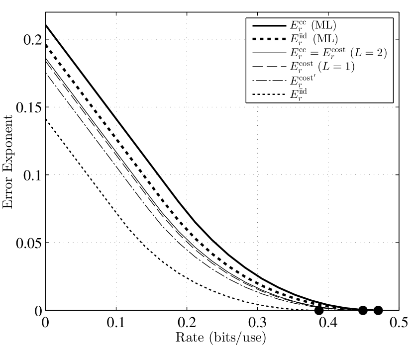
Figure 1: Error exponents for the channel defined in (56) with $\delta_{0}=0.01$, $\delta_{1}=0.05$, $\delta_{2}=0.25$ and $Q=(0.1,0.3,0.6)$. The mismatched decoder uses the minimum Hamming distance metric. The corresponding achievable rates $I_{\mathrm{GMI}}(Q)$, $I_{\mathrm{LM}}(Q)$ and $I(X;Y)$ are respectively marked on the horizontal axis.

IV Second-Order Coding Rates

In the matched setting, the finite-length performance limits of a channel are characterized by $M^{*}(n,\epsilon)$, defined to be the maximum number of codewords of length $n$ yielding an error probability not exceeding $\epsilon$ for some encoder and decoder. The problem of finding the second-order asymptotics of $M^{*}(n,\epsilon)$ for a given $\epsilon$ was studied by Strassen [10], and later revisited by Polyanskiy et al. [11] and Hayashi [12], among others. For DMCs, we have under mild technical conditions that

$$\log M^{*}(n,\epsilon)=nC-\sqrt{nV}\,\mathsf{Q}^{-1}(\epsilon)+O(\log n),$$ (57)

where $C$ is the channel capacity, and $V$ is known as the channel dispersion. Results of the form (57) provide a quantification of the speed of convergence to the channel capacity as the block length increases.

In this section, we present achievable second-order coding rates for the ensembles given in Section I, i.e. expansions of the form (57) with the equality replaced by $\geq$. To distinguish between the ensembles, we define $M^{\mathrm{iid}}(Q,n,\epsilon)$, $M^{\mathrm{cc}}(Q,n,\epsilon)$ and $M^{\mathrm{cost}}(Q,n,\epsilon)$ to be the maximum number of codewords of length $n$ such that the random-coding error probability does not exceed $\epsilon$ for the i.i.d., constant-composition and cost-constrained ensembles respectively, using the input distribution $Q$. We first consider the discrete memoryless setting, and then discuss more general memoryless channels.

IV-A Cost-Constrained Ensemble

A key quantity in the second-order analysis for ML decoding is the information density, given by

$$i(x,y)\triangleq\log\frac{W(y|x)}{\sum_{x}Q(x)W(y|x)},$$ (58)

where $Q$ is a given input distribution. In the mismatched setting, the relevant generalization of $i(x,y)$ is

$$i_{s,a}(x,y)\triangleq\log\frac{q(x,y)^{s}e^{a(x)}}{\sum_{\overline{x}}Q(\overline{x})q(\overline{x},y)^{s}e^{a(\overline{x})}},$$ (59)

where $s\geq 0$ and $a(\cdot)$ are fixed parameters. We write $i_{s,a}^{n}(\boldsymbol{x},\boldsymbol{y})\triangleq\sum_{i=1}^{n}i_{s,a}(x_{i},y_{i})$ and similarly $Q^{n}(\boldsymbol{x})\triangleq\prod_{i=1}^{n}Q(x_{i})$ and $a^{n}(\boldsymbol{x})\triangleq\sum_{i=1}^{n}a(x_{i})$. We define

$$I_{s,a}(Q) \triangleq\mathbb{E}[i_{s,a}(X,Y)]$$ (60)

$$U_{s,a}(Q) \triangleq\mathrm{Var}[i_{s,a}(X,Y)]$$ (61)

$$V_{s,a}(Q) \triangleq\mathbb{E}\big{[}\mathrm{Var}[i_{s,a}(X,Y)\,|\,X]\big{]},$$ (62)

where $(X,Y)\sim Q\times W$. From (9), we see that the LM rate is equal to $I_{s,a}(Q)$ after optimizing $s$ and $a(\cdot)$.

We can relate (60)–(62) with the $E_{0}$ functions defined in (35) and (39). Letting $E_{0}^{\mathrm{cost}^{\prime}}(Q,\rho,s,a)$ and $E_{0}^{\mathrm{cc}}(Q,\rho,s,a)$ denote the corresponding objectives with fixed $(s,a)$ in place of the supremum, we have $I_{s,a}=\frac{\partial E_{0}^{\mathrm{cost}^{\prime}}}{\partial\rho}\Big{|}_{\rho=0}=\frac{\partial E_{0}^{\mathrm{cc}}}{\partial\rho}\Big{|}_{\rho=0}$, $U_{s,a}=-\frac{\partial^{2}E_{0}^{\mathrm{cost}^{\prime}}}{\partial\rho^{2}}\Big{|}_{\rho=0}$, and $V_{s,a}=-\frac{\partial^{2}E_{0}^{\mathrm{cc}}}{\partial\rho^{2}}\Big{|}_{\rho=0}$. The latter two identities generalize a well-known connection between the exponent and dispersion in the matched case [11, p. 2337].

The main result of this subsection is the following theorem, which considers the cost-constrained ensemble. Our proof differs from the usual proof using threshold-based random-coding bounds [10, 11], but the latter approach can also be used in the present setting [30]. Our analysis can be interpreted as performing a normal approximation of $\mathrm{rcu}_{s}$ in (14).

Theorem 5.

Fix the input distribution $Q$ and the parameters $s\geq 0$ and $a(\cdot)$. Using the cost-constrained ensemble in (18) with $L=2$ and

$$a_{1}(x) =a(x)$$ (63)

$$a_{2}(x) =\mathbb{E}_{W(\cdot|x)}[i_{s,a}(x,Y)],$$ (64)

the following expansion holds:

$$\log M^{\mathrm{cost}}(Q,n,\epsilon)\geq nI_{s,a}(Q)-\sqrt{nV_{s,a}(Q)}\mathsf{Q}^{-1}(\epsilon)+O(\log n).$$ (65)

Proof.

Throughout the proof, we make use of the random variables $(X,Y,\overline{X})\sim Q(x)W(y|x)Q(\overline{x})$ and $(\boldsymbol{X},\boldsymbol{Y},\overline{\boldsymbol{X}})\sim P_{\boldsymbol{X}}(\boldsymbol{x})W^{n}(\boldsymbol{y}|\boldsymbol{x})P_{\boldsymbol{X}}(\overline{\boldsymbol{x}})$. Probabilities, expectations, etc. containing a realization $\boldsymbol{x}$ of $\boldsymbol{X}$ are implicitly defined to be conditioned on the event $\boldsymbol{X}=\boldsymbol{x}$.

We start with Theorem 1 and weaken $\mathrm{rcu}_{s}$ in (14) as follows:

$$\mathrm{rcu}_{s}(n,M)$$

$$=\mathbb{E}\bigg{[}\min\bigg{\{}1,(M-1)\frac{\sum_{\overline{\boldsymbol{x}}\in\mathcal{D}_{n}}P_{\boldsymbol{X}}(\overline{\boldsymbol{x}})q^{n}(\overline{\boldsymbol{X}},\boldsymbol{Y})^{s}}{q^{n}(\boldsymbol{X},\boldsymbol{Y})^{s}}\bigg{\}}\bigg{]}$$ (66)

$$\leq\mathbb{E}\bigg{[}\min\bigg{\{}1,Me^{2\delta}\frac{\sum_{\overline{\boldsymbol{x}}\in\mathcal{D}_{n}}P_{\boldsymbol{X}}(\overline{\boldsymbol{x}})q^{n}(\overline{\boldsymbol{X}},\boldsymbol{Y})^{s}e^{a^{n}(\overline{\boldsymbol{X}})}}{q^{n}(\boldsymbol{X},\boldsymbol{Y})^{s}e^{a^{n}(\boldsymbol{X})}}\bigg{\}}\bigg{]}$$ (67)

$$\leq\mathbb{E}\bigg{[}\min\bigg{\{}1,\frac{Me^{2\delta}}{\mu_{n}}\frac{\sum_{\overline{\boldsymbol{x}}}Q^{n}(\overline{\boldsymbol{x}})q^{n}(\overline{\boldsymbol{X}},\boldsymbol{Y})^{s}e^{a^{n}(\overline{\boldsymbol{X}})}}{q^{n}(\boldsymbol{X},\boldsymbol{Y})^{s}e^{a^{n}(\boldsymbol{X})}}\bigg{\}}\bigg{]}$$ (68)

$$=\mathbb{P}\bigg{[}i_{s,a}^{n}(\boldsymbol{X},\boldsymbol{Y})+\log U\leq\log\frac{Me^{2\delta}}{\mu_{n}}\bigg{]}$$ (69)

$$\leq\mathbb{P}\bigg{[}i_{s,a}^{n}(\boldsymbol{X},\boldsymbol{Y})+\log U\leq\log\frac{Me^{2\delta}}{\mu_{n}}\,\cap\,\boldsymbol{X}\in\mathcal{A}_{n}\bigg{]}$$

$$\qquad\qquad\qquad\qquad\qquad\qquad\qquad\qquad+\mathbb{P}\big{[}\boldsymbol{X}\notin\mathcal{A}_{n}\big{]}$$ (70)

$$\leq\max_{\boldsymbol{x}\in\mathcal{A}_{n}}\mathbb{P}\bigg{[}i_{s,a}^{n}(\boldsymbol{x},\boldsymbol{Y})+\log U\leq\log\frac{Me^{2\delta}}{\mu_{n}}\bigg{]}+\mathbb{P}\big{[}\boldsymbol{X}\notin\mathcal{A}_{n}\big{]},$$ (71)

where (67) follows from (31), (68) follows by substituting the random-coding distribution in (18) and summing over all $\overline{\boldsymbol{x}}$ instead of $\overline{\boldsymbol{x}}\in\mathcal{D}_{n}$, and (69) follows from the definition of $i^{n}_{s,a}$ and the identity

$$\mathbb{E}[\min\{1,A\}]=\mathbb{P}[A>U],$$ (72)

where $A$ is an arbitrary non-negative random variable, and $U$ is uniform on $(0,1)$ and independent of $A$. Finally, (70) holds for any set $\mathcal{A}_{n}$ by the law of total probability.

We treat the cases $V_{s,a}(Q)>0$ and $V_{s,a}(Q)=0$ separately. In the former case, we choose

$$\mathcal{A}_{n}=\bigg{\{}\boldsymbol{x}\in\mathcal{D}_{n}\,:\,\Big{|}\frac{1}{n}v_{s,a}^{n}(\boldsymbol{x})-V_{s,a}(Q)\Big{|}\leq\zeta\sqrt{\frac{\log n}{n}}\bigg{\}},$$ (73)

where $\zeta$ is a constant, and $v_{s,a}^{n}(\boldsymbol{x})\triangleq\sum_{i=1}^{n}v_{s,a}(x_{i})$ with

$$v_{s,a}(x)\triangleq\mathrm{Var}_{W(\cdot|x)}[i_{s,a}(x,Y)].$$ (74)

Using this definition along with that of $\mathcal{D}_{n}$ in (19) and the cost function in (64), we have for any $\boldsymbol{x}\in\mathcal{A}_{n}$ that

$$\Big{|}\mathbb{E}[i_{s,a}^{n}(\boldsymbol{x},\boldsymbol{Y})]-nI_{s,a}(Q)\Big{|} \leq\delta$$ (75)

$$\Big{|}\mathrm{Var}[i_{s,a}^{n}(\boldsymbol{x},\boldsymbol{Y})]-nV_{s,a}(Q)\Big{|} \leq\zeta\sqrt{n\log n},$$ (76)

for all $\boldsymbol{x}\in\mathcal{D}_{n}$. Since $\log U$ has finite moments, this implies

$$\Big{|}\mathbb{E}[i_{s,a}^{n}(\boldsymbol{x},\boldsymbol{Y})+\log U]-nI_{s,a}(Q)\Big{|} =O(1)$$ (77)

$$\Big{|}\mathrm{Var}[i_{s,a}^{n}(\boldsymbol{x},\boldsymbol{Y})+\log U]-nV_{s,a}(Q)\Big{|} =O\big{(}\sqrt{n\log n}\big{)}.$$ (78)

Using (18) and defining $\boldsymbol{X}^{\prime}\sim Q^{n}(\boldsymbol{x}^{\prime})$, we have

$$\mathbb{P}\big{[}\boldsymbol{X}\notin\mathcal{A}_{n}\big{]}\leq\frac{1}{\mu_{n}}\mathbb{P}\big{[}\boldsymbol{X}^{\prime}\notin\mathcal{A}_{n}\big{]}.$$ (79)

We claim that there exists a choice of $\zeta$ such that the right-hand side of (79) behaves as $O\big{(}\frac{1}{\sqrt{n}}\big{)}$, thus yielding

$$\mathbb{P}\big{[}\boldsymbol{X}\notin\mathcal{A}_{n}\big{]}=O\Big{(}\frac{1}{\sqrt{n}}\Big{)}.$$ (80)

Since Proposition 1 states that $\mu_{n}=\Omega(n^{-L/2})$, it suffices to show that $\mathbb{P}[\boldsymbol{X}^{\prime}\notin\mathcal{A}_{n}]$ can be made to behave as $O(n^{-(L+1)/2})$. This follows from the following moderate deviations result of [31, Thm. 2]: Given an i.i.d. sequence $\{Z_{i}\}_{i=1}^{n}$ with $\mathbb{E}[Z_{i}]=\mu$ and $\mathrm{Var}[Z_{i}]=\sigma^{2}>0$, we have $\mathbb{P}\big{[}\big{|}\frac{1}{n}\sum_{i=1}^{n}Z_{i}-\mu\big{|}>\eta\sigma\sqrt{\frac{\log n}{n}}\big{]}\asymp\frac{2}{\eta\sqrt{2\pi\log n}}n^{-\eta^{2}/2}$ provided that $\mathbb{E}[Z_{i}^{\eta^{2}+2+\delta}]<\infty$ for some $\delta>0$. The latter condition is always satisfied in the present setting, since we are considering finite alphabets.

We are now in a position to apply the Berry-Esseen theorem for independent and non-identically distributed random variables [32, Sec. XVI.5]. The relevant first and second moments are bounded in (77)–(78), and the relevant third moment is bounded since we are considering finite alphabets. Choosing

$$\log M=nI_{s,a}(Q)-\log\mu_{n}-2\delta-\xi_{n}$$ (81)

for some $\xi_{n}$, and also using (71) and (80), we obtain from the Berry-Esseen theorem that

$$\overline{p}_{e}\leq\mathsf{Q}\Bigg{(}\frac{\xi_{n}+O(1)}{\sqrt{nV_{s,a}(Q)+O(\sqrt{n\log n})}}\Bigg{)}+O\Big{(}\frac{1}{\sqrt{n}}\Big{)}.$$ (82)

By straightforward rearrangements and a first-order Taylor expansion of the square root function and the $\mathsf{Q}^{-1}$ function, we obtain

$$\xi_{n}\leq\sqrt{nV_{s,a}(Q)}\,\mathsf{Q}^{-1}(\overline{p}_{e})+O\big{(}\sqrt{\log n}\big{)}.$$ (83)

The proof for the case $V_{s,a}(Q)>0$ is concluded by combining (81) and (83), and noting from Proposition 1 that $\log\mu_{n}=O(\log n)$.

In the case that $V_{s,a}(Q)=0$, we can still make use of (77), but the variance is handled differently. From the definition in (62), we in fact have $\mathrm{Var}[i_{s,a}(x,Y)]=0$ for all $x$ such that $Q(x)>0$. Thus, for all $\boldsymbol{x}\in\mathcal{D}_{n}$ we have $\mathrm{Var}[i_{s,a}^{n}(\boldsymbol{x},\boldsymbol{Y})]=0$ and hence $\mathrm{Var}[i_{s,a}^{n}(\boldsymbol{x},\boldsymbol{Y})+\log U]=O(1)$. Choosing $M$ as in (81) and setting $\mathcal{A}_{n}=\mathcal{D}_{n}$, we can write (71) as

$$\mathrm{rcu}_{s}(n,M) \leq\max_{\boldsymbol{x}\in\mathcal{D}_{n}}\mathbb{P}\big{[}i_{s,a}^{n}(\boldsymbol{x},\boldsymbol{Y})+\log U-nI_{s,a}(Q)\leq-\xi_{n}\big{]}$$ (84)

$$\leq\frac{O(1)}{(\xi_{n}-O(1))^{2}},$$ (85)

where (85) holds due to (77) and Chebyshev’s inequality provided that $\xi_{n}$ is sufficiently large so that the $\xi_{n}-O(1)$ term is positive. Rearranging, we see that we can achieve any target value $\overline{p}_{e}=\epsilon$ with $\xi_{n}=O(1)$. The proof is concluded using (81). ∎

Theorem 5 can easily be extended to channels with more general alphabets. However, some care is needed, since the moderate deviations result [31, Thm. 2] used in the proof requires finite moments up to a certain order depending on $\zeta$ in (73). In the case that all moments of $i_{s,a}(X,Y)$ are finite, the preceding analysis is nearly unchanged, except that the third moment should be bounded in the set $\mathcal{A}_{n}$ in (73) in the same way as the second moment. An alternative approach is to introduce two further auxiliary costs into the ensemble:

$$a_{3}(x) =v_{s,a}(x)$$ (86)

$$a_{4}(x) =\mathbb{E}\big{[}|i_{s,a}(x,Y)-I_{s,a}(Q)|^{3}\big{]},$$ (87)

where $v_{s,a}$ is defined in (74). Under these choices, the relevant second and third moments for the Berry-Esseen theorem are bounded within $\mathcal{D}_{n}$ similarly to (77). The only further requirement is that the sixth moment of $i_{s,a}(X,Y)$ is finite under $Q\times W$, in accordance with Proposition 1.

We can easily deal with additive input constraints by handling them similarly to the auxiliary costs (see Section VI for details). With these modifications, our techniques provide, to our knowledge, the most general known second-order achievability proof for memoryless input-constrained channels with infinite or continuous alphabets. In particular, for the additive white Gaussian noise (AWGN) channel with a maximal power constraint and ML decoding, setting $s=1$ and $a(\cdot)=0$ yields the achievability part of the dispersion given by Polyanskiy et al. [11], thus providing a simple alternative to the proof therein based on the $\kappa\beta$ bound.

IV-B i.i.d. and Constant-Composition Ensembles

The properties of the cost-constrained ensemble used in the proof of Theorem 5 are also satisfied by the constant-composition ensemble, so we conclude that (65) remains true when $M^{\mathrm{cost}}$ is replaced by $M^{\mathrm{cc}}$. However, using standard bounds on $\mu_{n}$ in (71) (e.g. [14, p. 17]), we obtain a third-order $O(\log n)$ term which grows linearly in $|\mathcal{X}|$. In contrast, by Proposition 1 and (81), the cost-constrained ensemble yields a third-order term of the form $-\frac{L}{2}\log n+O(1)$, where $L$ is independent of $|\mathcal{X}|$.

The second-order asymptotic result for i.i.d. coding does not follow directly from Theorem 5, since the proof requires the cost function in (64) to be present. However, using similar arguments along with the identities $\mathbb{E}[i_{s}^{n}(\boldsymbol{X},\boldsymbol{Y})]=nI_{s}(Q)$ and $\mathrm{Var}[i_{s}^{n}(\boldsymbol{X},\boldsymbol{Y})]=nU_{s}(Q)$ (where $\boldsymbol{X}\sim Q^{n}$), we obtain

$$\log M^{\mathrm{iid}}(Q,n,\epsilon)\geq nI_{s}(Q)-\sqrt{nU_{s}(Q)}\,\mathsf{Q}^{-1}(\epsilon)+O(1)$$ (88)

for $s\geq 0$, where $I_{s}(Q)$ and $U_{s}(Q)$ are defined as in (60)–(61) with $a(\cdot)=0$. Under some technical conditions, the $O(1)$ term in (88) can be improved to $\frac{1}{2}{\log n}+O(1)$ using the techniques of [33, Sec. 3.4.5]; see Section V-C for further discussion.

IV-C Number of Auxiliary Costs Required

For ML decoding ($q(x,y)=W(y|x)$), we immediately see that $a_{1}(\cdot)$ in (63) is not needed, since the parameters maximizing $I_{s,a}(Q)$ in (60) are $s=1$ and $a(\cdot)=0$, thus yielding the mutual information.

We claim that, for any decoding metric, the auxiliary cost $a_{2}(\cdot)$ in (64) is not needed in the case that $Q$ and $a(\cdot)$ are optimized in (65). This follows from the following observation proved in Appendix -C: Given $s>0$, any pair $(Q,a)$ which maximizes $I_{s,a}(Q)$ must be such that $\mathbb{E}_{W(\cdot|x)}[i_{s,a}(x,Y)]$ has the same value for all $x$ such that $Q(x)>0$. Stated differently, the conditional variance $V_{s,a}(Q)$ coincides with the unconditional variance $U_{s,a}(Q)$ after the optimization of the parameters, thus generalizing the analogous result for ML decoding [11].

We observe that the number of auxiliary costs in each case coincides with that of the random-coding exponent (see Section III-C): $L=2$ suffices in general, $L=1$ suffices if the metric or input distribution is optimized, and $L=0$ suffices is both are optimized.

V Saddlepoint Approximations

Random-coding error exponents can be thought of as providing an estimate of the error probability of the form $p_{e}\approx e^{-nE_{r}(R)}$. More refined estimates can be obtained having the form $p_{e}\approx\alpha_{n}(R)e^{-nE_{r}(R)}$, where $\alpha_{n}(R)$ is a subexponential prefactor. Early works on characterizing the subexponential prefactor for a given rate under ML decoding include those of Elias [23] and Dobrushin [34], who studied specific channels exhibiting a high degree of symmetry. More recently, Altuğ and Wagner [22, 35] obtained asymptotic prefactors for arbitrary DMCs.

In this section, we take an alternative approach based on the saddlepoint approximation [13]. Our goal is to provide approximations for $\mathrm{rcu}$ and $\mathrm{rcu}_{s}$ (see Theorem 1) which are not only tight in the limit of large $n$ for a fixed rate, but also when the rate varies. In particular, our analysis will cover the regime of a fixed target error probability, which was studied in Section IV, as well as the moderate deviations regime, which was studied in [36, 37]. We focus on i.i.d. random coding, which is particularly amenable to a precise asymptotic analysis.

V-A Preliminary Definitions and Results

Analogously to Section IV, we fix $Q$ and $s>0$ and define the quantities

$$i_{s}(x,y) \triangleq\log\frac{q(x,y)^{s}}{\sum_{\overline{x}}Q(\overline{x})q(\overline{x},y)^{s}}$$ (89)

$$i_{s}^{n}(\boldsymbol{x},\boldsymbol{y}) \triangleq\sum_{i=1}^{n}i_{s}(x_{i},y_{i})$$ (90)

$$I_{s}(Q) \triangleq\mathbb{E}[i_{s}(X,Y)]$$ (91)

$$U_{s}(Q) \triangleq\mathrm{Var}[i_{s}(X,Y)],$$ (92)

where $(X,Y)\sim Q\times W$. We write $\mathrm{rcu}_{s}$ in (14) (with $P_{\boldsymbol{X}}=Q^{n}$) as

$$\mathrm{rcu}_{s}(n,M)=\mathbb{E}\Big{[}\min\big{\{}1,(M-1)e^{-i_{s}^{n}(\boldsymbol{X},\boldsymbol{Y})}\big{\}}\Big{]}.$$ (93)

We let

$$E_{0}^{\mathrm{iid}}(Q,\rho,s)\triangleq-\log\mathbb{E}\big{[}e^{-\rho i_{s}(X,Y)}\big{]}$$ (94)

denote the objective in (37) with a fixed value of $s$ in place of the supremum. The optimal value of $\rho$ is given by

$$\hat{\rho}(Q,R,s)\triangleq\operatorname*{arg\,max}_{\rho\in[0,1]}E_{0}^{\mathrm{iid}}(Q,\rho,s)-\rho R.$$ (95)

and the critical rate is defined as

$$R_{s}^{\mathrm{cr}}(Q)\triangleq\sup\big{\{}R\,:\,\hat{\rho}(Q,R,s)=1\big{\}}.$$ (96)

Furthermore, we define the following derivatives associated with (95):

$$c_{1}(Q,R,s) \triangleq R-\frac{\partial E_{0}^{\mathrm{iid}}(Q,\rho,s)}{\partial\rho}\bigg{|}_{\rho=\hat{\rho}(Q,R,s)}$$ (97)

$$c_{2}(Q,R,s) \triangleq-\frac{\partial^{2}E_{0}^{\mathrm{iid}}(Q,\rho,s)}{\partial\rho^{2}}\bigg{|}_{\rho=\hat{\rho}(Q,R,s)},$$ (98)

The following properties of the above quantities are analogous to those of Gallager for ML decoding [9, pp. 141-143], and can be proved in a similar fashion:

1. For all $R\geq 0$, we have $c_{2}(Q,R,s)>0$ if $U_{s}(Q)>0$, and $c_{2}(Q,R,s)=0$ if $U_{s}(Q)=0$. Furthermore, we have $c_{2}(Q,I_{s}(Q),s)=U_{s}(Q)$.

2. If $U_{s}(Q)=0$, then $R_{s}^{\mathrm{cr}}(Q)=I_{s}(Q)$.

3. For $R\in\big{[}0,R_{s}^{\mathrm{cr}}(Q)\big{)}$, we have $\hat{\rho}(Q,R,s)=1$ and $c_{1}(Q,R,s)<0$.

4. For $R\in\big{[}R_{s}^{\mathrm{cr}}(Q),I_{s}(Q)\big{]}$, $\hat{\rho}(Q,R,s)$ is strictly decreasing in $R$, and $c_{1}(Q,R,s)=0$.

5. For $R>I_{s}(Q)$, we have $\hat{\rho}(Q,R,s)=0$ and $c_{1}(Q,R,s)>0$.

Throughout this section, the arguments to $\hat{\rho}$, $c_{1}$, etc. will be omitted, since their values will be clear from the context.

The density function of a $N(\mu,\sigma^{2})$ random variable is denoted by

$$\phi(z;\mu,\sigma^{2})\triangleq\frac{1}{\sqrt{2\pi\sigma^{2}}}e^{-\frac{(z-\mu)^{2}}{2\sigma^{2}}}.$$ (99)

When studying lattice random variables (see Footnote 1 on Page 1) with span $h$, it will be useful to define

$$\phi_{h}(z;\mu,\sigma^{2})\triangleq\frac{h}{\sqrt{2\pi\sigma^{2}}}e^{-\frac{(z-\mu)^{2}}{2\sigma^{2}}},$$ (100)

which can be interpreted as an approximation of the integral of $\phi(\,\cdot\,;\mu,\sigma^{2})$ from $z$ to $z+h$ when $h$ is small.

V-B Approximation for $\mathrm{rcu}_{s}(n,M)$

In the proof of Theorem 6 below, we derive an approximation $\widehat{\mathrm{rcu}}_{s}$ of $\mathrm{rcu}_{s}$ taking the form

$$\widehat{\mathrm{rcu}}_{s}(n,M)\triangleq\alpha_{n}(Q,R,s)e^{-n(E_{0}^{\mathrm{iid}}(Q,\hat{\rho},s)-\hat{\rho}R)},$$ (101)

where $R=\frac{1}{n}\log M$, and the prefactor $\alpha_{n}$ varies depending on whether $i_{s}(X,Y)$ is a lattice variable. In the non-lattice case, the prefactor is given by

$$\alpha^{\mathrm{nl}}_{n}(Q,R,s)\triangleq\int_{0}^{\infty}e^{-\hat{\rho}z}\phi(z;nc_{1},nc_{2})dz\\ +\int_{-\infty}^{0}e^{(1-\hat{\rho})z}\phi(z;nc_{1},nc_{2})dz.$$ (102)

In the lattice case, it will prove convenient to deal with $R-i_{s}(X,Y)$ rather than $i_{s}(X,Y)$. Denoting the offset and span of $R-i_{s}(X,Y)$ by $\gamma$ and $h$ respectively, we see that $nR-i_{s}^{n}(\boldsymbol{X},\boldsymbol{Y})$ has span $h$, and its offset can be chosen as

$$\gamma_{n}\triangleq\min\Big{\{}n\gamma+ih\,:\,i\in\mathbb{Z},n\gamma+ih\geq 0\Big{\}}.$$ (103)

The prefactor for the lattice case is given by

$$\alpha^{\mathrm{l}}_{n}(Q,R,s)\triangleq\sum_{i=0}^{\infty}e^{-\hat{\rho}(\gamma_{n}+ih)}\phi_{h}(\gamma_{n}+ih;nc_{1},nc_{2})\\ +\sum_{i=-\infty}^{-1}e^{(1-\hat{\rho})(\gamma_{n}+ih)}\phi_{h}(\gamma_{n}+ih;nc_{1},nc_{2}),$$ (104)

and the overall prefactor in (101) is defined as

$$\alpha_{n}\triangleq\begin{cases}\alpha^{\mathrm{nl}}_{n}&i_{s}(X,Y)\text{ is non-lattice}\\ \alpha^{\mathrm{l}}_{n}&R-i_{s}(X,Y)\text{ has offset $\gamma$ and span $h$}.\end{cases}$$ (105)

While (102) and (104) are written in terms of integrals and summations, both prefactors can be computed efficiently to a high degree of accuracy. In the non-lattice case, this is easily done using the identity

$$\int_{a}^{\infty}e^{bz}\phi(z;\mu,\sigma^{2})dz=e^{\mu b+\frac{1}{2}\sigma^{2}b^{2}}\mathsf{Q}\Big{(}\frac{a-\mu-b\sigma^{2}}{\sigma}\Big{)}.$$ (106)

In the lattice case, we can write each of the summations in (104) in the form

$$\sum_{i}e^{b_{0}+b_{1}i+b_{2}i^{2}}=e^{-\frac{b_{1}^{2}}{4b_{2}}+b_{0}}\sum_{i}e^{b_{2}(i+\frac{b_{1}}{2b_{2}})^{2}},\\$$ (107)

where $b_{2}<0$. We can thus obtain an accurate approximation by keeping only the terms in the sum such that $i$ is sufficiently close to $-\frac{b_{1}}{2b_{2}}$. Overall, the computational complexity of the saddlepoint approximation is similar to that of the exponent alone.

Theorem 6.

Consider a DMC $W$, decoding metric $q$, input distribution $Q$, and parameter $s>0$ such that $U_{s}(Q)>0$. For any sequence $\{M_{n}\}$ such that $M_{n}\to\infty$, we have

$$\lim_{n\to\infty}\frac{\widehat{\mathrm{rcu}}_{s}(n,M_{n})}{\mathrm{rcu}_{s}(n,M_{n})}=1.$$ (108)

Proof:

See Appendix -E. ∎

A heuristic derivation of the non-lattice version of $\widehat{\mathrm{rcu}}_{s}$ was provided in [38]; Theorem 6 provides a formal derivation, along with a treatment of the lattice case. It should be noted that the assumption $U_{s}(Q)>0$ is not restrictive, since in the case that $U_{s}(Q)=0$ the argument to the expectation in (93) is deterministic, and hence $\mathrm{rcu}_{s}$ can easily be computed exactly.

In the case that the rate $R$ is fixed, simpler asymptotic expressions can be obtained. In Appendix -D, we prove the following (here $f_{n}\asymp g_{n}$ denotes the relation $\lim_{n\to\infty}\frac{f_{n}}{g_{n}}=1$):

• If $R\in[0,R_{s}^{\mathrm{cr}}(Q))$ or $R>I_{s}(Q)$, then

  $$\alpha_{n}(Q,R,s)\asymp 1.$$ (109)

• If $R=R_{s}^{\mathrm{cr}}(Q)$ or $R=I_{s}(Q)$, then

  $$\alpha_{n}(Q,R,s)\asymp\frac{1}{2}.$$ (110)

• If $R\in(R_{s}^{\mathrm{cr}}(Q),I_{s}(Q))$, then

  $$\alpha^{\mathrm{nl}}_{n}(Q,R,s) \asymp\frac{1}{\sqrt{2\pi nc_{2}}\hat{\rho}(1-\hat{\rho})}$$ (111)

  $$\alpha^{\mathrm{l}}_{n}(Q,R,s) \asymp\frac{h}{\sqrt{2\pi nc_{2}}}$$

  $$\times\Bigg{(}e^{-\hat{\rho}\gamma_{n}}\bigg{(}\frac{1}{1-e^{-\hat{\rho}h}}\bigg{)}+e^{(1-\hat{\rho})\gamma_{n}}\bigg{(}\frac{e^{-(1-\hat{\rho})h}}{1-e^{-(1-\hat{\rho})h}}\bigg{)}\Bigg{)}.$$ (112)

The asymptotic prefactors in (109)–(112) are related to the problem of exact asymptotics in the statistics literature, which seeks to characterize the subexponential prefactor for probabilities that decay at an exponential rate (e.g. see [39]). These prefactors are useful in gaining further insight into the behavior of the error probability compared to the error exponent alone. However, there is a notable limitation which is best demonstrated here using (111). The right-hand side of (111) characterizes the prefactor to within a multiplicative $1+o(1)$ term for a given rate, but it diverges as $\hat{\rho}\to 0$ or $\hat{\rho}\to 1$. Thus, unless $n$ is large, the estimate obtained by omitting the higher-order terms is inaccurate for rates slightly above $R_{s}^{\mathrm{cr}}(Q)$ or slightly below $I_{s}(Q)$.

In contrast, the right-hand side of (102) (and similarly (104)) remains bounded for all $\hat{\rho}\in[0,1]$. Furthermore, as Theorem 6 shows, this expression characterizes the true behavior of $\mathrm{rcu}_{s}$ to within a multiplicative $1+o(1)$ term not only for fixed rates, but also when the rate varies with the block length. Thus, it remains suitable for characterizing the behavior of $\mathrm{rcu}_{s}$ even when the rate approaches $R_{s}^{\mathrm{cr}}(Q)$ or $I_{s}(Q)$. In particular, this implies that $\widehat{\mathrm{rcu}}_{s}$ gives the correct second-order asymptotics of the rate for a given target error probability (see (88)). More precisely, the proof of Theorem 6 reveals that $\widehat{\mathrm{rcu}}_{s}=\mathrm{rcu}_{s}+O\big{(}\frac{1}{\sqrt{n}}\big{)}$, which implies (via a Taylor expansion of $\mathsf{Q}^{-1}$ in (88)) that the two yield the same asymptotics for a given error probability up to the $O(1)$ term.

V-C Approximation for $\mathrm{rcu}(n,M)$

In the proof of Theorem 1, we obtained $\mathrm{rcu}_{s}$ from $\mathrm{rcu}$ using Markov’s inequality. In this subsection we will see that, under some technical assumptions, a more refined analysis yields a bound which is tighter than $\mathrm{rcu}_{s}$, but still amenable to the techniques of the previous subsection.

V-C1 Technical Assumptions

Defining the set

$$\mathcal{Y}_{1}(Q)\triangleq\Big{\{}y\,:\,q(x,y)\neq q(\overline{x},y)\text{ for some }\\ x,\overline{x}\text{ such that }Q(x)Q(\overline{x})W(y|x)W(y|\overline{x})>0\Big{\}},$$ (113)

the technical assumptions on $(W,q,Q)$ are as follows:

$$q(x,y)>0\iff W(y|x)>0$$ (114)

$$\mathcal{Y}_{1}(Q)\neq\emptyset.$$ (115)

When $q(x,y)=W(y|x)$, (114) is trivial, and (115) is the non-singularity condition of [22]. A notable example where this condition fails is the binary erasure channel (BEC) with $Q=\big{(}\frac{1}{2},\frac{1}{2}\big{)}$. It should be noted that if (114) holds but (115) fails then we in fact have $\mathrm{rcu}=\mathrm{rcu}_{s}$ for any $s>0$, and hence $\widehat{\mathrm{rcu}}_{s}$ also approximates $\mathrm{rcu}$. This can be seen by noting that $\mathrm{rcu}_{s}$ is obtained from $\mathrm{rcu}$ using the inequality $\leavevmode\hbox{\small 1\normalsize\kern-3.30002pt1}\{\overline{q}\geq q\}\leq\big{(}\frac{\overline{q}}{q}\big{)}^{s}$, which holds with equality when $\frac{\overline{q}}{q}\in\{0,1\}$.

V-C2 Definitions

Along with the definitions in Section V-A, we will make use of the reverse conditional distribution

$$\widetilde{P}_{s}(x|y) \triangleq\frac{Q(x)q(x,y)^{s}}{\sum_{\overline{x}}Q(\overline{x})q(\overline{x},y)^{s}},$$ (116)

the joint tilted distribution

$$P_{\hat{\rho},s}^{*}(x,y)=\frac{Q(x)W(y|x)e^{-\hat{\rho}i_{s}(x,y)}}{\sum_{x^{\prime},y^{\prime}}Q(x^{\prime})W(y^{\prime}|x^{\prime})e^{-\hat{\rho}i_{s}(x^{\prime},y^{\prime})}},$$ (117)

and its $Y$-marginal $P_{\hat{\rho},s}^{*}(y)$, and the conditional variance

$$c_{3}(Q,R,s)\triangleq\mathbb{E}\Big{[}\mathrm{Var}\big{[}i_{s}(X^{*}_{s},Y_{s}^{*})\big{|}Y_{s}^{*}\big{]}\Big{]},$$ (118)

where $(X_{s}^{*},Y_{s}^{*})\sim P_{\hat{\rho},s}^{*}(y)\widetilde{P}_{s}(x|y)$. Furthermore, we define

$$\mathcal{I}_{s}\triangleq\Big{\{}i_{s}(x,y)\,:\,Q(x)W(y|x)>0,y\in\mathcal{Y}_{1}(Q)\Big{\}}$$ (119)

and let

$$\psi_{s}\triangleq\begin{cases}1&\mathcal{I}_{s}\text{ does not lie on a lattice}\\ \frac{\overline{h}}{1-e^{-\overline{h}}}&\mathcal{I}_{s}\text{ lies on a lattice with span }\overline{h}.\end{cases}$$ (120)

The set $\mathcal{I}_{s}$ is the support of a random variable which will appear in the analysis of the inner probability in (13). While $\overline{h}$ in (120) can differ from $h$ (the span of $i_{s}(X,Y)$) in general, the two coincide whenever $\mathcal{Y}_{1}(Q)=\mathcal{Y}$.

We claim that the assumptions in (114)–(115) imply that $c_{3}>0$ for any $R$ and $s>0$. To see this, we write

$$\mathrm{Var}_{\widetilde{P}_{s}(\cdot|y)}[i_{s}(X,y)]=0$$

$$\iff\log\frac{\widetilde{P}_{s}(x|y)}{Q(x)}\text{ is independent of }x\text{ where }\widetilde{P}_{s}(x|y)>0$$ (121)

$$\iff q(x,y)\text{ is independent of }x\text{ where }Q(x)q(x,y)>0$$ (122)

$$\iff y\notin\mathcal{Y}_{1}(Q),$$ (123)

where (121) and (122) follow from the definition of $\widetilde{P}_{s}$ in (116) and the assumption $s>0$, and (123) follows from (114) and the definition of $\mathcal{Y}_{1}(Q)$ in (113). Using (89), (114) and (117), we have

$$P_{\hat{\rho},s}^{*}(y)>0\iff\sum_{x}Q(x)W(y|x)>0.$$ (124)

Thus, from (115), we have $P^{*}_{\hat{\rho},s}(y)>0$ for some $y\in\mathcal{Y}_{1}(Q)$, which (along with (123)) proves that $c_{3}>0$.

V-C3 Main Result

The main result of this subsection is written in terms of an approximation of the form

$$\widehat{\mathrm{rcu}}_{s}^{*}(n,M)\triangleq\beta_{n}(Q,R,s)e^{-n(E_{0}^{\mathrm{iid}}(Q,\hat{\rho},s)-\hat{\rho}R)}.$$ (125)

Analogously to the previous subsection, we treat the lattice and non-lattice cases separately, writing

$$\beta_{n}\triangleq\begin{cases}\beta^{\mathrm{nl}}_{n}&i_{s}(X,Y)\text{ is non-lattice}\\ \beta^{\mathrm{l}}_{n}&R-i_{s}(X,Y)\text{ has offset $\gamma$ and span $h$},\end{cases}$$ (126)

where

$$\beta^{\mathrm{nl}}_{n}(Q,R,s)\triangleq\int_{\log\frac{\sqrt{2\pi nc_{3}}}{\psi_{s}}}^{\infty}e^{-\hat{\rho}z}\phi(z;nc_{1},nc_{2})dz$$

$$+\frac{\psi_{s}}{\sqrt{2\pi nc_{3}}}\int_{-\infty}^{\log\frac{\sqrt{2\pi nc_{3}}}{\psi_{s}}}e^{(1-\hat{\rho})z}\phi(z;nc_{1},nc_{2})dz$$ (127)

$$\beta^{\mathrm{l}}_{n}(Q,R,s)\triangleq\sum_{i=i^{*}}^{\infty}e^{-\hat{\rho}(\gamma_{n}+ih)}\phi_{h}(\gamma_{n}+ih;nc_{1},nc_{2})$$

$$+\frac{\psi_{s}}{\sqrt{2\pi nc_{3}}}\sum_{i=-\infty}^{i^{*}-1}e^{(1-\hat{\rho})(\gamma_{n}+ih)}\phi_{h}(\gamma_{n}+ih;nc_{1},nc_{2}),$$ (128)

and where in (128) we use $\gamma_{n}$ in (103) along with

$$i^{*}\triangleq\min\bigg{\{}i\in\mathbb{Z}\,:\,\gamma_{n}+ih\geq\log\frac{\sqrt{2\pi nc_{3}}}{\psi_{s}}\bigg{\}}.$$ (129)

Theorem 7.

Under the setup of Theorem 6 and the assumptions in (114)–(115), we have for any $s>0$ that

$$\mathrm{rcu}(n,M_{n})\leq\mathrm{rcu}_{s}^{*}(n,M_{n})(1+o(1)),$$ (130)

where

$$\mathrm{rcu}_{s}^{*}(n,M)\triangleq\mathbb{E}\bigg{[}\min\bigg{\{}1,\frac{M\psi_{s}}{\sqrt{2\pi nc_{3}}}e^{-i_{s}^{n}(\boldsymbol{X},\boldsymbol{Y})}\bigg{\}}\bigg{]}.$$ (131)

Furthermore, we have

$$\lim_{n\to\infty}\frac{\widehat{\mathrm{rcu}}_{s}^{*}(n,M_{n})}{\mathrm{rcu}_{s}^{*}(n,M_{n})}=1.$$ (132)

Proof:

See Appendix -F. ∎

When the rate does not vary with $n$, we can apply the same arguments as those given in Appendix -D to obtain the following analogues of (109)–(112):

• If $R\in[0,R_{s}^{\mathrm{cr}}(Q))$, then

  $$\beta_{n}(Q,R,s) \asymp\frac{\psi_{s}}{\sqrt{2\pi nc_{3}}},$$ (133)

  and similarly for $R=R_{s}^{\mathrm{cr}}(Q)$ after multiplying the right-hand side by $\frac{1}{2}$.

• If $R\in(R_{s}^{\mathrm{cr}}(Q),I_{s}(Q))$, then

  $$\beta^{\mathrm{nl}}_{n}(Q,R,s) \asymp\bigg{(}\frac{\psi_{s}}{\sqrt{2\pi nc_{3}}}\bigg{)}^{\hat{\rho}}\frac{1}{\sqrt{2\pi nc_{2}}\hat{\rho}(1-\hat{\rho})}$$ (134)

  $$\beta^{\mathrm{l}}_{n}(Q,R,s) \asymp\bigg{(}\frac{\psi_{s}}{\sqrt{2\pi nc_{3}}}\bigg{)}^{\hat{\rho}}\frac{h}{\sqrt{2\pi nc_{2}}}$$

  $$\times\Bigg{(}e^{-\hat{\rho}\gamma^{\prime}_{n}}\bigg{(}\frac{1}{1-e^{-\hat{\rho}h}}\bigg{)}+e^{(1-\hat{\rho})\gamma^{\prime}_{n}}\bigg{(}\frac{e^{-(1-\hat{\rho})h}}{1-e^{-(1-\hat{\rho})h}}\bigg{)}\Bigg{)},$$ (135)

  where $\gamma^{\prime}_{n}\triangleq\gamma_{n}+i^{*}h-\log\frac{\sqrt{2\pi nc_{3}}}{\psi_{s}}\in[0,h)$ (see (129)).

• For $R\geq I_{s}(Q)$, the asymptotics of $\beta_{n}$ coincide with those of $\alpha_{n}$ (see (109)–(110)).

When combined with Theorem 7, these expansions provide an alternative proof of the main result of [22], along with a characterization of the multiplicative $\Theta(1)$ terms which were left unspecified in [22]. A simpler version of the analysis in this paper can also be used to obtain the prefactors with unspecified constants; see [40] for details.

Analogously to the previous section, in the regime of fixed error probability we can write (132) more precisely as $\widehat{\mathrm{rcu}}_{s}^{*}=\mathrm{rcu}_{s}^{*}+O\big{(}\frac{1}{\sqrt{n}}\big{)}$, implying that the asymptotic expansions of the rates corresponding to $\mathrm{rcu}_{s}^{*}$ and $\widehat{\mathrm{rcu}}_{s}^{*}$ coincide up to the $O(1)$ term. From the analysis given in [33, Sec. 3.4.5], $\mathrm{rcu}_{s}^{*}$ yields an expansion of the form (88) with the $O(1)$ term replaced by $\frac{1}{2}\log{n}+O(1)$. It follows that the same is true of $\widehat{\mathrm{rcu}}_{s}^{*}$.

V-D Numerical Examples

Here we provide numerical examples to demonstrate the utility of the saddlepoint approximations given in this section. Along with $\widehat{\mathrm{rcu}}_{s}$ and $\widehat{\mathrm{rcu}}_{s}^{*}$, we consider (i) the normal approximation, obtained by omitted the remainder term in (88), (ii) the error exponent approximation $p_{e}\approx e^{-nE_{r}^{\mathrm{iid}}(Q,R)}$, and (iii) exact asymptotics approximations, obtained by ignoring the implicit $1+o(1)$ terms in (112) and (135). We use the lattice-type versions of the approximations, since we consider examples in which $i_{s}(X,Y)$ is a lattice variable. We observed no significant difference in the accuracy of each approximation in similar non-lattice examples.

We consider the example given in Section III-D, using the parameters $\delta_{0}=0.01$, $\delta_{1}=0.05$, $\delta_{2}=0.25$, and $Q=(\frac{1}{3},\frac{1}{3},\frac{1}{3})$. For the saddlepoint approximations, we approximate the summations of the form (107) by keeping the 1000 terms whose indices are closest to $-\frac{b_{1}}{2b_{2}}$. We choose the free parameter $s$ to be the value which maximizes the error exponent at each rate. For the normal approximation, we choose to $s$ achieve the GMI in (11). Defining $R^{\mathrm{cr}}(Q)$ to be the supremum of all rates such that $\hat{\rho}=1$ when $s$ is optimized, we have $I_{\mathrm{GMI}}(Q)=0.643$ and $R^{\mathrm{cr}}(Q)=0.185$ bits/use.

In Figure 2, we plot the error probability as a function of the rate with $n=60$. Despite the fact that the block length is small, we observe that $\mathrm{rcu}_{s}$ and $\widehat{\mathrm{rcu}}_{s}^{*}$ are indistinguishable at all rates. Similarly, the gap from $\mathrm{rcu}$ to $\widehat{\mathrm{rcu}}_{s}^{*}$ is small. Consistent with the fact that Theorem 7 gives an asymptotic upper bound on $\mathrm{rcu}$ rather than an asymptotic equality, $\widehat{\mathrm{rcu}}_{s}^{*}$ lies slightly above $\mathrm{rcu}$ at low rates. The error exponent approximation is close to $\mathrm{rcu}_{s}$ at low rates, but it is pessimistic at high rates. The normal approximation behaves somewhat similarly to $\mathrm{rcu}_{s}$, but it is less precise than the saddlepoint approximation, particularly at low rates.

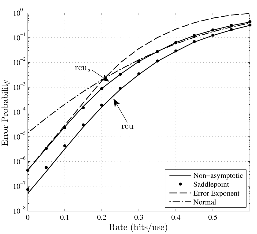
Figure 2: i.i.d. random-coding bounds for the channel defined in (56) with minimum Hamming distance decoding. The parameters are $n=60$, $\delta_{0}=0.01$, $\delta_{1}=0.05$, $\delta_{2}=0.25$ and $Q=(\frac{1}{3},\frac{1}{3},\frac{1}{3})$.

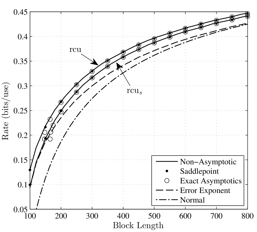
Figure 3: Rate required to achieve a target error probability $\epsilon$ for the channel defined in (56) with ML decoding. The parameters are $\epsilon=10^{-8}$, $\delta_{0}=\delta_{1}=\delta_{2}=\delta=0.1$ and $Q=(\frac{1}{3},\frac{1}{3},\frac{1}{3})$.

To facilitate the computation of $\mathrm{rcu}$ and $\mathrm{rcu}_{s}$ at larger block lengths, we consider the symmetric setup of $\delta_{0}=\delta_{1}=\delta_{2}=\delta=0.1$ and $Q=\big{(}\frac{1}{3},\frac{1}{3},\frac{1}{3}\big{)}$. Under these parameters, we have $I(X;Y)=0.633$ and $R^{\mathrm{cr}}(Q)=0.192$ bits/use. In Figure 3, we plot the rate required for each random-coding bound and approximation to achieve a given error probability $\epsilon=10^{-8}$, as a function of $n$. Once again, $\widehat{\mathrm{rcu}}_{s}$ is indistinguishable from $\mathrm{rcu}_{s}$, and similarly for $\widehat{\mathrm{rcu}}_{s}^{*}$ and $\mathrm{rcu}$. The error exponent approximation yields similar behavior to $\mathrm{rcu}_{s}$ at small block lengths, but the gap widens at larger block lengths. The exact asymptotics approximations are accurate other than a divergence near the critical rate, which is to be expected from the discussion in Section V-B. In contrast to similar plots with larger target error probabilities (e.g. [11, Fig. 8]), the normal approximation is inaccurate over a wide range of rates.

VI Discussion and Conclusion

We have introduced a cost-constrained ensemble with multiple auxiliary costs which yields similar performance gains to constant-composition coding, while remaining applicable in the case of infinite or continuous alphabets. We have studied the number of auxiliary costs required to match the performance of the constant-composition ensemble, and shown that the number can be reduced when the input distribution or decoding metric is optimized. Using the saddlepoint approximation, refined asymptotic estimates have been given for the i.i.d. ensemble which unify the regimes of error exponents, second-order rates and moderate deviations, and provide accurate approximations of the random-coding bounds.

Extension to Channels with Input Constraints

Suppose that each codeword $\boldsymbol{x}$ is constrained to satisfy $\frac{1}{n}\sum_{i=1}^{n}c(x_{i})\leq\Gamma$ for some (system) cost function $c(\cdot)$. The i.i.d. ensemble is no longer suitable, since in all non-trivial cases it has a positive probability of producing codewords which violate the constraint. On the other hand, the results for the constant-composition ensemble remain unchanged provided that $Q$ itself satisfies the cost constraint, i.e. $\sum_{x}Q(x)c(x)\leq\Gamma$.

For the cost-constrained ensemble, the extension is less trivial but still straightforward. The main change required is a modification of the definition of $\mathcal{D}_{n}$ in (19) to include a constraint on the quantity $\frac{1}{n}\sum_{i=1}^{n}c(x_{i})$. Unlike the auxiliary costs in (19), where the sample mean can be above or below the true mean, the system cost of each codeword is constrained to be less than or equal to its mean. That is, the additional constraint is given by

$$\frac{1}{n}\sum_{i=1}^{n}c(x_{i})\leq\phi_{c}\triangleq\sum_{x}Q(x)c(x),$$ (136)

or similarly with both upper and lower bounds (e.g. $-\frac{\delta}{n}\leq\frac{1}{n}\sum_{i=1}^{n}c(x_{i})-\phi_{c}\leq 0$). Using this modified definition of $\mathcal{D}_{n}$, one can prove the subexponential behavior of $\mu_{n}$ in Proposition 1 provided that $Q$ is such that $\phi_{c}\leq\Gamma$, and the exponents and second-order rates for the cost-constrained ensemble remain valid under any such $Q$.

-A Proof of Theorem 2

The proof is similar to that of Gallager for the constant-composition ensemble [15], so we omit some details. The codeword distribution in (18) can be written as

$$P_{\boldsymbol{X}}(\boldsymbol{x})=\frac{1}{\mu_{n}}\prod_{i=1}^{n}Q(x_{i})\leavevmode\hbox{\small 1\normalsize\kern-3.30002pt1}\big{\{}\hat{P}_{\boldsymbol{x}}\in\mathcal{G}_{n}\big{\}},$$ (137)

where $\hat{P}_{\boldsymbol{x}}$ is the empirical distribution (type) of $\boldsymbol{x}$, and $\mathcal{G}_{n}$ is the set of types corresponding to sequences $\boldsymbol{x}\in\mathcal{D}_{n}$ (see (19)). We define the sets

$$\mathcal{S}_{n}(\mathcal{G}_{n})\triangleq\big{\{}P_{XY}\in\mathcal{P}_{n}(\mathcal{X}\times\mathcal{Y})\,:\,P_{X}\in\mathcal{G}_{n}\big{\}}$$ (138)

$$\mathcal{T}_{n}(P_{XY},\mathcal{G}_{n})\triangleq\big{\{}\widetilde{P}_{XY}\in\mathcal{P}_{n}(\mathcal{X}\times\mathcal{Y})\,:\,\widetilde{P}_{X}\in\mathcal{G}_{n},\\ \widetilde{P}_{Y}=P_{Y},\mathbb{E}_{\widetilde{P}}[\log q(X,Y)]\geq\mathbb{E}_{P}[\log q(X,Y)]\big{\}}.$$ (139)

We have from Theorem 1 that $\overline{p}_{e}\doteq\mathrm{rcu}$. Expanding $\mathrm{rcu}$ in terms of types, we obtain

$$\overline{p}_{e}\doteq\sum_{P_{XY}\in\mathcal{S}_{n}(\mathcal{G}_{n})}\mathbb{P}\big{[}(\boldsymbol{X},\boldsymbol{Y})\in T^{n}(P_{XY})\big{]}\min\bigg{\{}1,\\ (M-1)\sum_{\widetilde{P}_{XY}\in\mathcal{T}_{n}(P_{XY},\mathcal{G}_{n})}\mathbb{P}\big{[}(\overline{\boldsymbol{X}},\boldsymbol{y})\in T^{n}(\widetilde{P}_{XY})\big{]}\bigg{\}},$$ (140)

where $\boldsymbol{y}$ denotes an arbitrary sequence with type $P_{Y}$.

From Proposition 1, the normalizing constant in (137) satisfies $\mu_{n}\doteq 1$, and thus we can safely proceed from (140) as if the codeword distribution were $P_{\boldsymbol{X}}=Q^{n}$. Using the property of types in [15, Eq. (18)], it follows that the two probabilities in (140) behave as $e^{-nD(P_{XY}\|Q\times W)}$ and $e^{-nD(\widetilde{P}_{XY}\|Q\times P_{Y})}$ respectively. Combining this with the fact that the number of joint types is polynomial in $n$, we obtain $\overline{p}_{e}\doteq e^{-nE_{r,n}(Q,R,\mathcal{G}_{n})}$, where

$$E_{r,n}(Q,R,\mathcal{G}_{n})\triangleq\min_{P_{XY}\in\mathcal{S}_{n}(\mathcal{G}_{n})}\min_{\widetilde{P}_{XY}\in\mathcal{T}_{n}(P_{XY},\mathcal{G}_{n})}\\ D(P_{XY}\|Q\times W)+\big{[}D(\widetilde{P}_{XY}\|Q\times P_{Y})-R\big{]}^{+}.$$ (141)

Using a simple continuity argument (e.g. see [28, Eq. (30)]), we can replace the minimizations over types by minimizations over joint distributions, and the constraints of the form $|\mathbb{E}_{P}[a_{l}(X)]-\phi_{l}|\leq\frac{\delta}{n}$ can be replaced by $\mathbb{E}_{P}[a_{l}(X)]=\phi_{l}$. This concludes the proof.

-B Proof of Theorem 3

Throughout the proof, we make use of Fan’s minimax theorem [41], which states that $\min_{a}\sup_{b}f(a,b)=\sup_{b}\min_{a}f(a,b)$ provided that the minimum is over a compact set, $f(\cdot,b)$ is convex in $a$ for all $b$, and $f(a,\cdot)$ is concave in $b$ for all $a$. We make use of Lagrange duality [17] in a similar fashion to [5, Appendix A]; some details are omitted to avoid repetition with [5].

Using the identity $[\alpha]^{+}=\max_{\rho\in[0,1]}\rho\alpha$ and Fan’s minimax theorem, the expression in (27) can be written as

$$E_{r}^{\mathrm{cc}}(Q,R)=\max_{\rho\in[0,1]}\hat{E}_{0}^{\mathrm{cc}}(Q,\rho)-\rho R,$$ (142)

where

$$\hat{E}_{0}^{\mathrm{cc}}(Q,\rho)\triangleq\min_{P_{XY}\in\mathcal{S}(\{a_{l}\})}\min_{\widetilde{P}_{XY}\in\mathcal{T}(P_{XY},\{a_{l}\})}\\ D(P_{XY}\|Q\times W)+\rho D(\widetilde{P}_{XY}\|Q\times P_{Y}).$$ (143)

It remains to show that $\hat{E}_{0}^{\mathrm{cc}}(Q,\rho)=E_{0}^{\mathrm{cc}}(Q,\rho)$. We will show this by considering the minimizations in (143) one at a time. We can follow the steps of [5, Appendix A] to conclude that

$$\min_{\widetilde{P}_{XY}\in\mathcal{T}(P_{XY},\{a_{l}\})}D(\widetilde{P}_{XY}\|Q\times P_{Y})=\sup_{s\geq 0,\{\overline{r}_{l}\}}\\ \sum_{x,y}P_{XY}(x,y)\log\frac{q(x,y)^{s}}{\sum_{\overline{x}}Q(\overline{x})q(\overline{x},y)^{s}e^{\sum_{l}\overline{r}_{l}(a_{l}(\overline{x})-\phi_{l})}},$$ (144)

where $s$ and $\{\overline{r}_{l}\}$ are Lagrange multipliers. It follows that the inner minimization in (143) is equivalent to

$$\min_{P_{XY}\in\mathcal{S}(\{a_{l}\})}\sup_{s\geq 0,\{\overline{r}_{l}\}}\sum_{x,y}P_{XY}(x,y)\Bigg{(}\log\frac{P_{XY}(x,y)}{Q(x)W(y|x)}\\ +\rho\log\frac{q(x,y)^{s}}{\sum_{\overline{x}}Q(\overline{x})q(\overline{x},y)^{s}e^{\sum_{l}\overline{r}_{l}(a_{l}(\overline{x})-\phi_{l})}}\Bigg{)}.$$ (145)

Since the objective is convex in $P_{XY}$ and jointly concave in $(s,\{\overline{r}_{l}\})$, we can apply Fan’s minimax theorem. Hence, we consider the minimization of the objective in (145) over $P_{XY}\in\mathcal{S}(\{a_{l}\})$ with $s$ and $\{\overline{r}_{l}\}$ fixed. Applying the techniques of [5, Appendix A] a second time, we conclude that this minimization has a dual form given by

$$\sup_{\{r_{l}\}}-\log\sum_{x,y}P_{XY}(x,y)\Bigg{(}\frac{\sum_{\overline{x}}Q(\overline{x})q(\overline{x},y)^{s}e^{\sum_{l}\overline{r}_{l}(a_{l}(\overline{x})-\phi_{l})}}{q(x,y)^{s}e^{\sum_{l}r_{l}(a_{l}(x)-\phi_{l})}}\Bigg{)}^{\rho},$$ (146)

where $\{r_{l}\}$ are Lagrange multipliers. The proof is concluded by taking the supremum over $s$ and $\{\overline{r}_{l}\}$.

-C Necessary Conditions for the Optimal Parameters

-C1 Optimization of $E_{0}^{\mathrm{cc}}(Q,\rho)$

We write the objective in (39) as

$$E_{0}^{\mathrm{cc}}(Q,\rho,s,a)\triangleq\rho\sum_{x}Q(x)a(x)-\sum_{x}Q(x)\log f(x),$$ (147)

where

$$f(x)\triangleq\sum_{y}W(y|x)q(x,y)^{-\rho s}\bigg{(}\sum_{\overline{x}}Q(\overline{x})q(\overline{x},y)^{s}e^{a(\overline{x})}\bigg{)}^{\rho}.$$ (148)

We have the partial derivatives

$$\frac{\partial f(x)}{\partial Q(x^{\prime})} =\rho g(x,x^{\prime})$$ (149)

$$\frac{\partial f(x)}{\partial a(x^{\prime})} =\rho Q(x^{\prime})g(x,x^{\prime}),$$ (150)

where

$$g(x,x^{\prime})\triangleq\sum_{y}W(y|x)q(x,y)^{-\rho s}\\ \times\rho\left(\sum_{\overline{x}}Q(\overline{x})q(\overline{x},y)^{s}e^{a(\overline{x})}\right)^{\rho-1}q(x^{\prime},y)^{s}e^{a(x^{\prime})}$$ (151)

We proceed by analyzing the necessary Karush-Kuhn-Tucker (KKT) conditions [17] for $(Q,a)$ to maximize $E_{0}^{\mathrm{cc}}(Q,\rho,s,a)$. The KKT condition corresponding to the partial derivative with respect to $a(x^{\prime})$ is

$$\rho Q(x^{\prime})-\sum_{x}Q(x)\frac{\rho Q(x^{\prime})g(x,x^{\prime})}{f(x)}=0,$$ (152)

or equivalently

$$\sum_{x}Q(x)\frac{g(x,x^{\prime})}{f(x)}=1.$$ (153)

Similarly, the KKT condition corresponding to $Q(x^{\prime})$ gives

$$\rho a(x^{\prime})-\log f(x^{\prime})-\rho\sum_{x}Q(x)\frac{g(x,x^{\prime})}{f(x)}-\lambda=0$$ (154)

for all $x^{\prime}$ such that $Q(x^{\prime})>0$, where $\lambda$ is the Lagrange multiplier associated with the constraint $\sum_{x}Q(x)=1$. Substituting (153) into (154) gives

$$-\log\big{(}f(x^{\prime})e^{-\rho a(x^{\prime})}\big{)}=\lambda+\rho.$$ (155)

Using the definition of $f(\cdot)$ in (148), we see that (155) implies that the logarithm in (39) is independent of $x$.

-C2 Optimization of $I_{s,a}(Q)$

We write $I_{s,a}(Q)$ in (60) as

$$I_{s,a}(Q)=s\sum_{x,y}Q(x)W(y|x)\log q(x,y)+\sum_{x}Q(x)a(x)\\ -\sum_{x,y}Q(x)W(y|x)\log\sum_{\overline{x}}Q(\overline{x})q(\overline{x},y)^{s}e^{a(\overline{x})}$$ (156)

and analyze the KKT conditions associated with the maximization over $(Q,a)$. We omit some details, since the steps are similar to those above. The KKT condition for $a(x^{\prime})$ is

$$\sum_{x,y}Q(x)W(y|x)\frac{q(x^{\prime},y)^{s}e^{a(x^{\prime})}}{\sum_{\overline{x}}Q(\overline{x})q(\overline{x},y)^{s}e^{a(\overline{x})}}=1,$$ (157)

and the KKT condition for $Q(x^{\prime})$ gives

$$s\sum_{y}W(y|x^{\prime})\log q(x^{\prime},y)+a(x^{\prime})$$

$$-\sum_{y}W(y|x^{\prime})\log\sum_{\overline{x}}Q(\overline{x})q(\overline{x},y)^{s}e^{a(\overline{x})}$$

$$-\sum_{x,y}Q(x)W(y|x)\frac{q(x^{\prime},y)^{s}e^{a(x^{\prime})}}{\sum_{\overline{x}}Q(\overline{x})q(\overline{x},y)^{s}e^{a(\overline{x})}}-\lambda=0$$ (158)

for all $x^{\prime}$ such that $Q(x^{\prime})>0$, where $\lambda$ is a Lagrange multiplier. Substituting (157) into (158) and performing some simple rearrangements, we obtain

$$\sum_{y}W(y|x^{\prime})\log\frac{q(x^{\prime},y)^{s}e^{a(x^{\prime})}}{\sum_{\overline{x}}Q(\overline{x})q(\overline{x},y)^{s}e^{a(\overline{x})}}=\lambda+1.$$ (159)

-D Asymptotic Behavior of the Saddlepoint Approximation

Here we prove the asymptotic relations given in (109)–(112). We will make frequent use of the properties of $\hat{\rho}$, $c_{1}$ and $c_{2}$ given in Section V-A.

We first prove (109)–(110) in the non-lattice case. Suppose that $R<R_{s}^{\mathrm{cr}}(Q)$, and hence $\hat{\rho}=1$, $c_{1}<0$ and $c_{2}>0$. Using (106) and the identity $\mathsf{Q}(z)\leq\frac{1}{2}\exp\big{(}\frac{-z^{2}}{2}\big{)}$ for $z>0$, it is easily verified that the first term in (102) decays to zero exponentially fast. The second term is given by $\mathsf{Q}\big{(}-c_{1}\sqrt{\frac{n}{c_{2}}}\big{)}$, which tends to one since $\lim_{z\to\infty}\mathsf{Q}(z)=1$. We thus obtain (109). When $R=R_{s}^{\mathrm{cr}}(Q)$, the argument is similar except that $c_{1}=0$, yielding the following: (i) From (106), the first term in (102) equals $\mathsf{Q}(\sqrt{nc_{2}})e^{nc_{2}/2}\asymp\frac{1}{\sqrt{2\pi nc_{2}}}$, rather than decaying exponentially fast, (ii) The second term in (102) equals $\mathsf{Q}(0)=\frac{1}{2}$, rather than one. For $R>I_{s}(Q)$ (respectively, $R=I_{s}(Q)$) the argument is similar with the roles of the two terms in (102) reversed, and with $\hat{\rho}=0$ and $c_{1}>0$ (respectively, $c_{1}=0$).

In the lattice case, the arguments in proving (109)–(110) are similar to the non-lattice case, so we focus on (109) with $R<R_{s}^{\mathrm{cr}}(Q)$. Similarly to the non-lattice case, it is easily shown that the first summation in (104) decays to zero exponentially fast, so we focus on the second. Since $\hat{\rho}=1$, the second summation is given by

$$\sum_{i=-\infty}^{-1}\phi_{h}(\gamma_{n}+ih;nc_{1},nc_{2})$$

$$\qquad=(1+o(1))\sum_{i=-\infty}^{\infty}\phi_{h}(\gamma_{n}+ih;nc_{1},nc_{2})$$ (160)

$$\qquad=1+o(1),$$ (161)

where (160) follows since the added terms from $i=0$ to $\infty$ contribute an exponentially small amount to the sum since $c_{1}<0$, and (161) is easily understood by interpreting the right-hand side of (160) as approximating the integral over the real line of a Gaussian density function via discrete sampling. Since the sampling is done using intervals of a fixed size $h$ but the variance $nc_{2}$ increases, the approximation improves with $n$ and approaches one.

Finally, we consider the case that $R\in(R_{s}^{\mathrm{cr}}(Q),I_{s}(Q))$, and hence $\hat{\rho}\in(0,1)$, $c_{1}=0$ and $c_{2}>0$. In the non-lattice case, we can substitute $c_{1}=0$ and (106) into (104) to obtain

$$\alpha_{n} =e^{\frac{1}{2}nc_{2}\hat{\rho}^{2}}\mathsf{Q}\big{(}\hat{\rho}\sqrt{nc_{2}}\big{)}+e^{\frac{1}{2}nc_{2}(1-\hat{\rho})^{2}}\mathsf{Q}\big{(}(1-\hat{\rho})\sqrt{nc_{2}}\big{)}.$$ (162)

Using the fact that $\mathsf{Q}(z)e^{z^{2}/2}\asymp\frac{1}{z\sqrt{2\pi}}$ as $z\to\infty$, along with the identity $\frac{1}{\rho}+\frac{1}{1-\rho}=\frac{1}{\rho(1-\rho)}$, we obtain (111).

We now turn to the lattice case. Setting $c_{1}=0$ in (104) yields

$$\alpha_{n}=\frac{h}{\sqrt{2\pi nc_{2}}}\bigg{(}\sum_{i=0}^{\infty}e^{-\hat{\rho}(\gamma_{n}+ih)-\frac{(\gamma_{n}+ih)^{2}}{2nc_{2}}}+\\ \sum_{i=-\infty}^{-1}e^{(1-\hat{\rho})(\gamma_{n}+ih)-\frac{(\gamma_{n}+ih)^{2}}{2nc_{2}}}\bigg{)}.$$ (163)

The two summations are handled in a nearly identical fashion, so we focus on the first. Using the identity $1-x\leq e^{-x}\leq 1$, we can write

$$\Bigg{|}\sum_{i=0}^{\infty}e^{-\hat{\rho}(\gamma_{n}+ih)-\frac{(\gamma_{n}+ih)^{2}}{2nc_{2}}}-\sum_{i=0}^{\infty}e^{-\hat{\rho}(\gamma_{n}+ih)}\Bigg{|}$$

$$\qquad\leq\sum_{i=0}^{\infty}e^{-\hat{\rho}(\gamma_{n}+ih)}\frac{(\gamma_{n}+ih)^{2}}{2nc_{2}}$$ (164)

$$\qquad=O\Big{(}\frac{1}{n}\Big{)},$$ (165)

where (165) follows since the summation $\sum_{i=0}^{\infty}e^{-\zeta i}p(i)$ is convergent for any polynomial $p(i)$ and $\zeta>0$. Furthermore, we have from the geometric series that

$$\sum_{i=0}^{\infty}e^{-\hat{\rho}(\gamma_{n}+ih)}=e^{-\hat{\rho}\gamma_{n}}\bigg{(}\frac{1}{1-e^{-\hat{\rho}h}}\bigg{)},$$ (166)

We have thus weakened the first summation in (163) to the first term in the sum in (112) (up to an $O\big{(}\frac{1}{n}\big{)}$ remainder term). The second term is obtained in a similar fashion.

-E Proof of Theorem 6

Since $M_{n}\to\infty$ by assumption, we can safely replace $M_{n}$ by $M_{n}+1$ without affecting the theorem statement. We begin by considering fixed values of $n$, $M$ and $R=\frac{1}{n}\log M$.

Using (93) and the identity in (72), we can can write

$$\mathrm{rcu}_{s}(n,M+1)=\mathbb{P}\bigg{[}nR-\sum_{i=1}^{n}i_{s}(X_{i},Y_{i})\geq\log U\bigg{]}.$$ (167)

This expression resembles the tail probability of an i.i.d. sum of random variables, for which asymptotic estimates were given by Bahadur and Rao [39] (see also [9, Appendix 5A]). There are two notable differences in our setting which mean that the results of [39, 9] cannot be applied directly. First, the right-hand side of the event in (167) random rather than deterministic. Second, since we are allowing for rates below $R_{s}^{\mathrm{cr}}(Q)$ or above $I_{s}(Q)$, we cannot assume that the derivative of the moment generating function of $R-i_{s}(X,Y)$ at zero (which we will shortly see equals $c_{1}$ in (97)) is equal to zero.

-E1 Alternative Expressions for $\mathrm{rcu}_{s}$

Let $F(t)$ denote the cumulative distribution function (CDF) of $R-i_{s}(X,Y)$, and let $Z_{1},\cdots,Z_{n}$ be i.i.d. according to the tilted CDF

$$F_{Z}(z)=e^{E_{0}^{\mathrm{iid}}(Q,\hat{\rho},s)-\hat{\rho}R}\int_{-\infty}^{z}e^{\hat{\rho}t}dF(t).$$ (168)

It is easily seen that this is indeed a CDF by writing

$$\int_{-\infty}^{\infty}e^{\hat{\rho}t}dF(t)=\mathbb{E}\big{[}e^{\hat{\rho}(R-i_{s}(X,Y))}\big{]}=e^{-(E_{0}^{\mathrm{iid}}(Q,\hat{\rho},s)-\hat{\rho}R)},$$ (169)

where we have used (94). The moment generating function (MGF) of $Z$ is given by

$$M_{Z}(\tau) \triangleq\mathbb{E}\big{[}e^{\tau Z}\big{]}$$ (170)

$$=e^{E_{0}^{\mathrm{iid}}(Q,\hat{\rho},s)-\hat{\rho}R}\mathbb{E}\big{[}e^{(\hat{\rho}+\tau)(R-i_{s}(X,Y))}\big{]}$$ (171)

$$=e^{E_{0}^{\mathrm{iid}}(Q,\hat{\rho},s)}e^{-(E_{0}^{\mathrm{iid}}(Q,\hat{\rho}+\tau,s)-\tau R)},$$ (172)

where (171) follows from (168), and (172) follows from (94). We can now compute the mean and variance of $Z$ in terms of the derivatives of the MGF, namely

$$\mathbb{E}[Z] =\frac{dM_{Z}}{d\tau}\Big{|}_{\tau=0}=c_{1}$$ (173)

$$\mathrm{Var}[Z] =\frac{d^{2}M_{Z}}{d\tau^{2}}\Big{|}_{\tau=0}-\mathbb{E}[Z]^{2}=c_{2},$$ (174)

where $c_{1}$ and $c_{2}$ are defined in (97)–(98). Recall that $U_{s}(Q)>0$ by assumption, which implies that $c_{2}>0$ (see Section V-A).

In the remainder of the proof, we omit the arguments $(Q,\hat{\rho},s)$ to $E_{0}^{\mathrm{iid}}$. Following [39, Lemma 2], we can use (168) to write (167) as follows:

$$\mathrm{rcu}_{s}(n,M+1)$$

$$\quad=\dotsint_{\sum_{i}t_{i}\geq\log u}dF(t_{1})\cdots dF(t_{n})dF_{U}(u)$$ (175)

$$\quad=e^{-n(E_{0}^{\mathrm{iid}}-\hat{\rho}R)}$$

$$\quad\,\,\,\times\dotsint_{\sum_{i}z_{i}\geq\log u}e^{-\hat{\rho}\sum_{i}z_{i}}dF_{Z}(z_{1})\cdots dF_{Z}(z_{n})dF_{U}(u),$$ (176)

$$\quad\triangleq I_{n}e^{-n(E_{0}^{\mathrm{iid}}-\hat{\rho}R)},$$ (177)

where $F_{U}(u)$ is the CDF of $U$. We write the prefactor $I_{n}$ as

$$I_{n}=\int_{0}^{1}\int_{\log u}^{\infty}e^{-\hat{\rho}z}dF_{n}(z)dF_{U}(u),$$ (178)

where $F_{n}$ is the CDF of $\sum_{i=1}^{n}Z_{i}$. Since the integrand in (178) is non-negative, we can safely interchange the order of integration, yielding

$$I_{n} =\int_{-\infty}^{\infty}\int_{0}^{\min\{1,e^{z}\}}e^{-\hat{\rho}z}dF_{U}(u)dF_{n}(z)$$ (179)

$$=\int_{0}^{\infty}e^{-\hat{\rho}z}dF_{n}(z)+\int_{-\infty}^{0}e^{(1-\hat{\rho})z}dF_{n}(z),$$ (180)

where (180) follows by splitting the integral according to which value achieves the $\min\{\cdot,\cdot\}$ in (179). Letting $\hat{F_{n}}$ denote the CDF of $\frac{\sum_{i=1}^{n}Z_{i}-nc_{1}}{\sqrt{nc_{2}}}$, we can write (180) as

$$I_{n}=\int_{-\frac{c_{1}\sqrt{n}}{\sqrt{c_{2}}}}^{\infty}e^{-\hat{\rho}(z\sqrt{nc_{2}}+nc_{1})}d\hat{F}_{n}(z)\\ +\int_{-\infty}^{-\frac{c_{1}\sqrt{n}}{\sqrt{c_{2}}}}e^{(1-\hat{\rho})(z\sqrt{nc_{2}}+nc_{1})}d\hat{F}_{n}(z).$$ (181)

-E2 Non-lattice Case

Let $\Phi(z)$ denote the CDF of a zero-mean unit-variance Gaussian random variable. Using the fact that $\mathbb{E}[Z]=c_{1}$ and $\mathrm{Var}[Z]=c_{2}>0$ (see (173)–(174)), we have from the refined central limit theorem in [32, Sec. XVI.4, Thm. 1] that

$$\hat{F}_{n}(z)=\Phi(z)+G_{n}(z)+\tilde{F}_{n}(z),$$ (182)

where $\tilde{F}_{n}(z)=o(n^{-\frac{1}{2}})$ uniformly in $z$, and

$$G_{n}(z)\triangleq\frac{K}{\sqrt{n}}(1-z^{2})e^{-\frac{1}{2}z^{2}}$$ (183)

for some constant $K$ depending only on the variance and third absolute moment of $Z$, the latter of which is finite since we are considering finite alphabets. Substituting (182) into (181), we obtain

$$I_{n}=I_{1,n}+I_{2,n}+I_{3,n},$$ (184)

where the three terms denote the right-hand side of (181) with $\Phi$, $G_{n}$ and $\tilde{F}_{n}$ respectively in place of $\hat{F}_{n}$. Reversing the step from (180) to (181), we see that $I_{1,n}$ is precisely $\alpha_{n}$ in (102). Furthermore, using $\frac{dG_{n}}{dz}=\frac{K}{\sqrt{n}}(z^{3}-3z)e^{-\frac{1}{2}z^{2}}$, we obtain

$$I_{2,n}=\frac{K}{\sqrt{n}}\bigg{(}\int_{-\frac{c_{1}\sqrt{n}}{\sqrt{c_{2}}}}^{\infty}e^{-\hat{\rho}(z\sqrt{nc_{2}}+nc_{1})}(z^{3}-3z)e^{-\frac{1}{2}z^{2}}dz\\ +\int_{-\infty}^{-\frac{c_{1}\sqrt{n}}{\sqrt{c_{2}}}}e^{(1-\hat{\rho})(z\sqrt{nc_{2}}+nc_{1})}(z^{3}-3z)e^{-\frac{1}{2}z^{2}}dz\bigg{)}.$$ (185)

In accordance with the theorem statement, we must show that $I_{2,n}=o(\alpha_{n})$ and $I_{3,n}=o(\alpha_{n})$ even in the case that $R$ and $\hat{\rho}$ vary with $n$. Let $R_{n}=\frac{1}{n}\log M_{n}$ and $\hat{\rho}_{n}=\hat{\rho}(Q,R_{n},s)$, and let $c_{1,n}$ and $c_{2,n}$ be the corresponding values of $c_{1}$ and $c_{2}$. We assume with no real loss of generality that

$$\lim_{n\to\infty}R_{n}=R^{*}$$ (186)

for some $R^{*}\geq 0$ possibly equal to $\infty$. Once the theorem is proved for all such $R^{*}$, the same will follow for an arbitrary sequence $\{R_{n}\}$.

Table I summarizes the growth rates $\alpha_{n}$, $I_{2,n}$ and $I_{3,n}$ for various ranges of $R^{*}$, and indicates whether the first or second integral (see (181) and (185)) dominates the behavior of each. We see that $I_{2,n}=o(\alpha_{n})$ and $I_{3,n}=o(\alpha_{n})$ for all values of $R^{*}$, as desired.

Table I: Growth rates of $\alpha_{n}$, $I_{2,n}$ and $I_{3,n}$ when the rate converges to $R^{*}$.

	$\hat{\rho}$	$c_{1}$	Dominant Term(s)	$\alpha_{n}$	$I_{2,n}$	$I_{3,n}$
$R^{*}\in[0,R_{s}^{\mathrm{cr}}(Q))$	$1$	$<0$	2	$\Theta(1)$	$\Theta\Big{(}\frac{1}{\sqrt{n}}\Big{)}$	$o\Big{(}\frac{1}{\sqrt{n}}\Big{)}$
$R^{*}=R_{s}^{\mathrm{cr}}(Q)$	$\to 1$	$\to 0$	2	$\omega\Big{(}\frac{1}{\sqrt{n}}\Big{)}$	$O\Big{(}\frac{1}{\sqrt{n}}\Big{)}$	$o\Big{(}\frac{1}{\sqrt{n}}\Big{)}$
$R^{*}\in(R_{s}^{\mathrm{cr}}(Q),I_{s}(Q))$	$\in(0,1)$	$0$	1,2	$\Theta\Big{(}\frac{1}{\sqrt{n}}\Big{)}$	$\Theta\Big{(}\frac{1}{n\sqrt{n}}\Big{)}$	$o\Big{(}\frac{1}{\sqrt{n}}\Big{)}$
$R^{*}=I_{s}(Q)$	$\to 0$	$\to 0$	1	$\omega\Big{(}\frac{1}{\sqrt{n}}\Big{)}$	$O\Big{(}\frac{1}{\sqrt{n}}\Big{)}$	$o\Big{(}\frac{1}{\sqrt{n}}\Big{)}$
$R^{*}>I_{s}(Q)$	$0$	$>0$	1	$\Theta(1)$	$\Theta\Big{(}\frac{1}{\sqrt{n}}\Big{)}$	$o\Big{(}\frac{1}{\sqrt{n}}\Big{)}$

The derivations of the growth rates in Table I when $R^{*}\notin\{R_{s}^{\mathrm{cr}}(Q),I_{s}(Q)\}$ are done in a similar fashion to Appendix -D. To avoid repetition, we provide details only for $R^{*}=R_{s}^{\mathrm{cr}}(Q)$; this is a less straightforward case whose analysis differs slightly from Appendix -D. From Section V-A, we have $\hat{\rho}\to 1$ and $c_{1,n}\to 0$ from below, with $c_{1,n}<0$ only if $\hat{\rho}_{n}=1$.

For any $\hat{\rho}\in[0,1]$, the terms $e^{-\hat{\rho}(\cdot)}$ and $e^{(1-\hat{\rho})(\cdot)}$ in (185) are both upper bounded by one across their respective ranges of integration. Since the moments of a Gaussian random variable are finite, it follows that both integrals are $O(1)$, and thus $I_{2,n}=O\big{(}\frac{1}{\sqrt{n}}\big{)}$. The term $I_{3,n}$ is handled similarly, so it only remains to show that $\alpha_{n}=\omega\big{(}\frac{1}{\sqrt{n}}\big{)}$. In the case that $\hat{\rho}=1$, the second integral in (102) is at least $\frac{1}{2}$, since $c_{1}\leq 0$. It only remains to handle the case that $c_{1}=0$ and $\hat{\rho}_{n}\to 1$ with $\hat{\rho}_{n}<1$. For any $\delta>0$, we have $\hat{\rho}_{n}\geq 1-\delta$ for sufficiently large $n$. Lower bounding $\alpha_{n}$ by replacing $1-\hat{\rho}$ by $\delta$ in the second term of (102), we have similarly to (162) that

$$\alpha_{n}\geq e^{\frac{1}{2}nc_{2}\delta^{2}}\mathsf{Q}\big{(}\delta\sqrt{nc_{2}}\big{)}\asymp\frac{1}{\sqrt{2\pi nc_{2}}\delta}.$$ (187)

Since $\delta$ is arbitrary, we obtain $\alpha_{n}=\omega\big{(}\frac{1}{\sqrt{n}}\big{)}$, as desired.

-E3 Lattice case

The arguments following (184) are essentially identical in the lattice case, so we focus our attention on obtaining the analogous expression to (184). Letting $P_{n}(z)$ denote the probability mass function (PMF) of $\sum_{i=1}^{n}Z_{i}$, we can write (180) as

$$I_{n}=\sum_{z\geq 0}P_{n}(z)e^{-\hat{\rho}z}+\sum_{z<0}P_{n}(z)e^{(1-\hat{\rho})z}.$$ (188)

Using the fact that $\mathbb{E}[Z]=c_{1}$ and $\mathrm{Var}[Z]=c_{2}>0$, we have from the local limit theorem in [9, Eq. (5A.12)] that

$$P_{n}(z)=\phi_{h}(z;nc_{1},nc_{2})+\tilde{P}_{n}(z),$$ (189)

where $\phi_{h}$ is defined in (100), and $\tilde{P}_{n}(z)=o\big{(}\frac{1}{\sqrt{n}}\big{)}$ uniformly in $z$. Thus, analogously to (184), we can write

$$I_{n}=I_{1,n}+I_{2,n},$$ (190)

where the two terms denote the right-hand side of (188) with $\phi_{h}$ and $\tilde{P}_{n}(z)$ respectively in place of $P_{n}(z)$. Using the definition of $\gamma_{n}$ in (103) and the fact that $\sum_{i}Z_{i}$ has the same support as $nR-i_{s}^{n}(\boldsymbol{X},\boldsymbol{Y})$ (cf. (168)), we see that the first summation in (188) is over the set $\{\gamma_{n}+ih:i\in\mathbb{Z},i\geq 0\}$, and the second summation is over the set $\{\gamma_{n}+ih:i\in\mathbb{Z},i<0\}$. It follows that $I_{1,n}=\alpha_{n}$, and similar arguments to the non-lattice case show that $I_{2,n}=o(\alpha_{n})$.

-F Proof of Theorem 7

Throughout this section, we make use of the same notation as Appendix -E. We first discuss the proof of (132). Using the definition of $\mathrm{rcu}_{s}^{*}$, we can follow identical arguments to those following (167) to conclude that

$$\mathrm{rcu}_{s}^{*}(n,M)=I_{n}e^{-n(E_{0}^{\mathrm{iid}}(Q,\hat{\rho},s)-\hat{\rho}R)},$$ (191)

where analogously to (178) and (180), we have

$$I_{n} =\int_{0}^{1}\int_{\log\frac{u\sqrt{2\pi nc_{3}}}{\psi_{s}}}^{\infty}e^{-\hat{\rho}z}dF_{n}(z)dF_{U}(u)$$ (192)

$$=\int_{\log\frac{\sqrt{2\pi nc_{3}}}{\psi_{s}}}^{\infty}e^{-\hat{\rho}z}dF_{n}(z)$$

$$\qquad\qquad+\frac{\psi_{s}}{\sqrt{2\pi nc_{3}}}\int_{-\infty}^{\log\frac{\sqrt{2\pi nc_{3}}}{\psi_{s}}}e^{(1-\hat{\rho})z}dF_{n}(z).$$ (193)

The remaining arguments in proving (132) follow those given in Appendix -E, and are omitted.

To prove (130), we make use of two technical lemmas, whose proofs are postponed until the end of the section. The following lemma can be considered a refinement of [11, Lemma 47].

Lemma 1.

Fix $K>0$, and for each $n$, let $(n_{1},\cdots,n_{K})$ be integers such that $\sum_{k}n_{k}=n$. Fix the PMFs $Q_{1},\cdots,Q_{K}$ on a finite subset of $\mathbb{R}$, and let $\sigma_{1}^{2},\cdots,\sigma_{K}^{2}$ be the corresponding variances. Let $Z_{1},\cdots,Z_{n}$ be independent random variables, $n_{k}$ of which are distributed according to $Q_{k}$ for each $k$. Suppose that $\min_{k}\sigma_{k}>0$ and $\min_{k}n_{k}=\Theta(n)$. Defining

$$\mathcal{I}_{0} \triangleq\bigcup_{k\,:\,\sigma_{k}>0}\big{\{}z\,:\,Q_{k}(z)>0\big{\}}$$ (194)

$$\psi_{0} \triangleq\begin{cases}1&\mathcal{I}_{0}\text{ \em does not lie on a lattice}\\ \frac{h_{0}}{1-e^{-h_{0}}}&\mathcal{I}_{0}\text{ \em lies on a lattice with span }h_{0},\end{cases}$$ (195)

the summation $S_{n}\triangleq\sum_{i}Z_{i}$ satisfies the following uniformly in $t$:

$$\mathbb{E}\Big{[}e^{-S_{n}}\emph{\leavevmode\hbox{\small 1\normalsize\kern-3.30002pt1}}\big{\{}S_{n}>t\big{\}}\Big{]}\leq e^{-t}\bigg{(}\frac{\psi_{0}}{\sqrt{2\pi V_{n}}}+o\Big{(}\frac{1}{\sqrt{n}}\Big{)}\bigg{)},$$ (196)

where $V_{n}\triangleq\mathrm{Var}[S_{n}]$.

Roughly speaking, the following lemma ensures the existence of a high probability set in which Lemma 1 can be applied to the inner probability in (13). We make use of the definitions in (116)–(118), and we define the random variables

$$(\boldsymbol{X},\boldsymbol{Y},\overline{\boldsymbol{X}},\boldsymbol{X}_{s})\sim Q^{n}(\boldsymbol{x})W^{n}(\boldsymbol{y}|\boldsymbol{x})Q^{n}(\overline{\boldsymbol{x}})\widetilde{P}_{s}^{n}(\boldsymbol{x}_{s}|\boldsymbol{y}),$$ (197)

where $\widetilde{P}_{s}^{n}(\boldsymbol{x}|\boldsymbol{y})\triangleq\prod_{i=1}^{n}\widetilde{P}_{s}(x_{i}|y_{i})$. Furthermore, we write the empirical distribution of $\boldsymbol{y}$ as $\hat{P}_{\boldsymbol{y}}$, and we let $P_{\boldsymbol{Y}}$ denote the PMF of $\boldsymbol{Y}$.

Lemma 2.

Let the parameters $s>0$ and $\hat{\rho}\in[0,1]$ be given. If the triplet $(W,q,Q)$ satisfies (114)–(115), then the set

$$\mathcal{F}_{\hat{\rho},s}^{n}(\delta)\triangleq\Big{\{}\boldsymbol{y}\,:\,P_{\boldsymbol{Y}}(\boldsymbol{y})>0,\,\max_{y}\big{|}\hat{P}_{\boldsymbol{y}}(y)-P_{\hat{\rho},s}^{*}(y)\big{|}\leq\delta\Big{\}}$$ (198)

satisfies the following properties:

1. For any $\boldsymbol{y}\in\mathcal{F}_{\hat{\rho},s}^{n}(\delta)$, we have

   $$\mathrm{Var}\big{[}i_{s}^{n}(\boldsymbol{X}_{s},\boldsymbol{Y})\,|\,\boldsymbol{Y}=\boldsymbol{y}\big{]}\geq n(c_{3}-r(\delta)),$$ (199)

   where $r(\delta)\to 0$ as $\delta\to 0$.

2. For any $\delta>0$, we have

   $$\liminf_{n\to\infty}-\frac{1}{n}\log\frac{\sum_{\boldsymbol{x},\boldsymbol{y}\notin\mathcal{F}_{\hat{\rho},s}^{n}(\delta)}Q^{n}(\boldsymbol{x})W^{n}(\boldsymbol{y}|\boldsymbol{x})e^{-\hat{\rho}i_{s}^{n}(\boldsymbol{x},\boldsymbol{y})}}{\sum_{\boldsymbol{x},\boldsymbol{y}}Q^{n}(\boldsymbol{x})W^{n}(\boldsymbol{y}|\boldsymbol{x})e^{-\hat{\rho}i_{s}^{n}(\boldsymbol{x},\boldsymbol{y})}}>0.$$ (200)

It should be noted that since the two statements of Lemma 2 hold true for any $\hat{\rho}\in[0,1]$, they also hold true when $\hat{\rho}$ varies within this range, thus allowing us to handle rates which vary with $n$. Before proving the lemmas, we show how they are used to obtain the desired result.

Proof of (130) based on Lemmas 1–2

By upper bounding $M-1$ by $M$ and splitting $\mathrm{rcu}$ (see (13)) according to whether or not $\boldsymbol{y}\in\mathcal{F}_{\hat{\rho},s}^{n}(\delta)$, we obtain

$$\mathrm{rcu}(n,M)\leq\sum_{\boldsymbol{x},\boldsymbol{y}\in\mathcal{F}_{\hat{\rho},s}^{n}(\delta)}Q^{n}(\boldsymbol{x})W^{n}(\boldsymbol{y}|\boldsymbol{x})$$

$$\qquad\qquad\qquad\times\min\Big{\{}1,M\mathbb{P}[i_{s}^{n}(\overline{\boldsymbol{X}},\boldsymbol{y})\geq i_{s}^{n}(\boldsymbol{x},\boldsymbol{y})]\Big{\}}$$

$$+M^{\hat{\rho}}\sum_{\boldsymbol{x},\boldsymbol{y}\notin\mathcal{F}_{\hat{\rho},s}^{n}(\delta)}Q^{n}(\boldsymbol{x})W^{n}(\boldsymbol{y}|\boldsymbol{x})e^{-\hat{\rho}i_{s}^{n}(\boldsymbol{x},\boldsymbol{y})},$$ (201)

where we have replaced $q^{n}$ by $i_{s}^{n}$ since each is a monotonically increasing function of the other, and in the summation over $\boldsymbol{y}\notin\mathcal{F}_{\hat{\rho},s}^{n}(\delta)$ we further weakened the bound using Markov’s inequality and $\min\{1,\cdot\}\leq(\cdot)^{\hat{\rho}}$. In order to make the inner probability in (201) more amenable to an application of Lemma 1, we follow [33, Sec. 3.4.5] and note that the following holds whenever $\widetilde{P}_{s}^{n}(\overline{\boldsymbol{x}}|\boldsymbol{y})>0$:

$$Q^{n}(\overline{\boldsymbol{x}}) =Q^{n}(\overline{\boldsymbol{x}})\frac{\widetilde{P}_{s}^{n}(\overline{\boldsymbol{x}}|\boldsymbol{y})}{\widetilde{P}_{s}^{n}(\overline{\boldsymbol{x}}|\boldsymbol{y})}=\widetilde{P}_{s}^{n}(\overline{\boldsymbol{x}}|\boldsymbol{y})e^{-i_{s}^{n}(\overline{\boldsymbol{x}},\boldsymbol{y})}.$$ (202)

For a fixed sequence $\boldsymbol{y}$ and a constant $t$, summing (202) over all $\overline{\boldsymbol{x}}$ such that $i_{s}^{n}(\overline{\boldsymbol{x}},\boldsymbol{y})\geq t$ yields

$$\mathbb{P}[i_{s}^{n}(\overline{\boldsymbol{X}},\boldsymbol{y})\geq t]=\mathbb{E}\Big{[}e^{-i_{s}^{n}(\boldsymbol{X}_{s},\boldsymbol{Y})}\leavevmode\hbox{\small 1\normalsize\kern-3.30002pt1}\big{\{}i_{s}^{n}(\boldsymbol{X}_{s},\boldsymbol{Y})\geq t\big{\}}\,\Big{|}\,\boldsymbol{Y}=\boldsymbol{y}\Big{]}$$ (203)

under the joint distribution in (197).

We now observe that (203) is of the same form as the left-hand side of (196). We apply Lemma 1 with $Q_{k}$ given by the PMF of $i_{s}(X_{s},y_{k})$ under $X_{s}\sim\widetilde{P}_{s}(\,\cdot\,|y_{k})$, where $y_{k}$ is the $k$-th output symbol for which $\sum_{x}Q(x)W(y|x)>0$. The conditions of the lemma are easily seen to be satisfied for sufficiently small $\delta$ due to the definition of $\mathcal{F}_{\hat{\rho},s}^{n}(\delta)$ in (198), the assumption in (115), and (123). We have from (196), (199) and (203) that

$$\mathbb{P}\big{[}i_{s}^{n}(\overline{\boldsymbol{X}},\boldsymbol{y})\geq t\big{]}\leq\frac{\psi_{s}}{\sqrt{2\pi n(c_{3}-r(\delta))}}e^{-t}(1+o(1))$$ (204)

for all $\boldsymbol{y}\in\mathcal{F}_{\hat{\rho},s}^{n}(\delta)$ and sufficiently small $\delta$. Here we have used the fact that $\psi_{0}$ in (195) coincides with $\psi_{s}$ in (120), which follows from (123) and the fact that $\widetilde{P}_{s}(x|y)>0$ if and only if $Q(x)W(y|x)>0$ (see (114) and (116)).

Using the uniformity of the $o(1)$ term in $t$ in (204) (see Lemma 1), taking $\delta\to 0$ (and hence $r(\delta)\to 0$), and writing

$$\min\{1,f_{n}(1+\zeta_{n})\}\leq(1+|\zeta_{n}|)\min\{1,f_{n}\},$$ (205)

we see that the first term in (201) is upper bounded by $\mathrm{rcu}_{s}^{*}(n,M)(1+o(1))$. To complete the proof of (130), we must show that the second term in (201) can be incorporated into the multiplicative $1+o(1)$ term. To see this, we note from (125) and (132) that the exponent of $\mathrm{rcu}_{s}^{*}$ is given by $E_{0}^{\mathrm{iid}}(Q,\hat{\rho},s)-\hat{\rho}R$. From (94), the denominator in the logarithm in (200) equals $e^{-nE_{0}^{\mathrm{iid}}(Q,\hat{\rho},s)}$. Combining these observations, the second part of Lemma 2 shows that the second term in (201) decays at a faster exponential rate than $\mathrm{rcu}_{s}^{*}$, thus yielding the desired result.

Proof of Lemma 1

The proof makes use of the local limit theorems given in [42, Thm. 1] and [43, Sec. VII.1, Thm. 2] for the non-lattice and lattice cases respectively. We first consider the summation $S^{\prime}_{n}\triangleq\sum_{i=1}^{n^{\prime}}Z_{i}$, where we assume without loss of generality that the first $n^{\prime}=\Theta(n)$ indices correspond to positive variances, and the remaining $n-n^{\prime}$ correspond to zero variances. We similarly assume that $\sigma_{k}>0$ for $k=1,\cdots,K^{\prime}$, and $\sigma_{k}=0$ for $k=K^{\prime}+1,\cdots,K$. We clearly have $\mathrm{Var}[S^{\prime}_{n}]=\mathrm{Var}[S_{n}]=V_{n}$.

We first consider the non-lattice case. We claim that the conditions of the lemma imply the following local limit theorem given in [42, Thm. 1]:

$$\mathbb{P}\big{[}S^{\prime}_{n}\in[z,z+\eta)\big{]}=\frac{\eta}{\sqrt{2\pi V_{n}}}e^{-\frac{(z-\mu^{\prime}_{n})^{2}}{2V_{n}}}+o\Big{(}\frac{1}{\sqrt{n}}\Big{)}$$ (206)

uniformly in $z$, where $\mu^{\prime}_{n}\triangleq\mathbb{E}[S^{\prime}_{n}]$, and $\eta>0$ is arbitrary. To show this, we must verify the technical assumptions given in [42, p. 593]. First, [42, Cond. ($\alpha$)] states that there exists $Z_{\mathrm{max}}<\infty$ and $c>0$ such that

$$\frac{1}{\mathrm{Var}[Z]}\mathbb{E}\big{[}(Z-\mathbb{E}[Z])^{2}\leavevmode\hbox{\small 1\normalsize\kern-3.30002pt1}\{|Z-\mathbb{E}[Z]|\leq Z_{\mathrm{max}}\}\big{]}>c$$ (207)

under $Z\sim Q_{k}$ and each $k=1,\cdots,K^{\prime}$. This is trivially satisfied since we are considering finite alphabets, which implies that the support of each $Q_{k}$ is bounded. The Lindeberg condition is stated in [42, Cond. ($\gamma$)], and is trivially satisfied due to the assumption that $n_{k}=\Theta(n)$ for all $k$. The only non-trivial condition is [42, Cond. ($\beta$)], which can be written as follows in the case of finite alphabets: For any given lattice, there exists $\delta>0$ such that

$$\frac{1}{\log V_{n}}\sum_{i=1}^{n^{\prime}}\mathbb{P}[Z_{i}\text{ is not }\delta\text{-close to a lattice point}]\to\infty.$$ (208)

Since we are considering the case that $\mathcal{I}_{0}$ does not lie on a lattice, we have for sufficiently small $\delta$ that the summation grows linearly in $n$, whereas $\log V_{n}$ only grows as $\log n$. We have thus shown that each of the technical conditions in [42] is satisfied, and hence (206) holds.

Upper bounding the exponential term in (206) by one, and noting that $S_{n}-S^{\prime}_{n}$ has zero variance, we obtain

$$\mathbb{P}\big{[}S_{n}\in[z,z+\eta)\big{]}\leq\frac{\eta}{\sqrt{2\pi V_{n}}}+o\Big{(}\frac{1}{\sqrt{n}}\Big{)}$$ (209)

uniformly in $z$. We can now prove the lemma similarly to [11, Lemma 47] by writing

$$\mathbb{E}\Big{[}e^{-S_{n}}\leavevmode\hbox{\small 1\normalsize\kern-3.30002pt1}\big{\{}S_{n}>t\big{\}}\Big{]}$$

$$\qquad\leq\sum_{l=0}^{\infty}e^{-t-l\eta}\mathbb{P}\Big{[}t+l\eta\leq S_{n}\leq t+(l+1)\eta\Big{]}$$ (210)

$$\qquad\leq\sum_{l=0}^{\infty}e^{-t-l\eta}\bigg{(}\frac{\eta}{\sqrt{2\pi V_{n}}}+o\Big{(}\frac{1}{\sqrt{n}}\Big{)}\bigg{)}$$ (211)

$$\qquad=e^{-t}\bigg{(}\frac{\eta}{(1-e^{-\eta})\sqrt{2\pi V_{n}}}+o\Big{(}\frac{1}{\sqrt{n}}\Big{)}\bigg{)},$$ (212)

where (212) follows by evaluating the summation using the geometric series. The proof is concluded by taking $\eta\to 0$ and using the identity $\lim_{\eta\to 0}\frac{\eta}{1-e^{-\eta}}=1$. The uniformity of (196) in $t$ follows from the uniformity of (209) in $z$.

In the lattice case, the argument is essentially unchanged, but we instead use the local limit theorem given in [43, Sec. VII.1, Thm. 2], which yields

$$\mathbb{P}[S^{\prime}_{n}=z]=\frac{h_{0}}{\sqrt{2\pi V_{n}}}e^{-\frac{(z-\mu^{\prime}_{n})^{2}}{2V_{n}}}+o\Big{(}\frac{1}{\sqrt{n}}\Big{)}$$ (213)

uniformly in $z$ on the lattice corresponding to $S^{\prime}_{n}$ (with span $h_{0}$). The remaining arguments are identical to the non-lattice case, with $\eta=h_{0}$ instead of $\eta\to 0$.

Proof of Lemma 2

We obtain (199) by using the definitions of $c_{3}$ and $\mathcal{F}_{\hat{\rho},s}^{n}(\delta)$ (see (118) and (198)) to write

$$\mathrm{Var}[i_{s}^{n}(\boldsymbol{X}_{s},\boldsymbol{Y})\,|\,\boldsymbol{Y}=\boldsymbol{y}]$$

$$\qquad=\sum_{y}n\hat{P}_{\boldsymbol{y}}(y)\mathrm{Var}[i_{s}^{n}(X_{s},Y)\,|\,Y=y]$$ (214)

$$\qquad\geq\sum_{y}n(P^{*}_{\hat{\rho},s}(y)-\delta)\mathrm{Var}[i_{s}^{n}(X_{s},Y)\,|\,Y=y]$$ (215)

$$\qquad=n\big{(}c_{3}-o(\delta)\big{)},$$ (216)

where $(X_{s}|Y=y)\sim\widetilde{P}_{s}(\,\cdot\,|\,y)$. To prove the second property, we perform an expansion in terms of types in the same way as Appendix -A to conclude that the exponent of the denominator in the logarithm in (200) is given by

$$\min_{P_{XY}}\sum_{x,y}P_{XY}(x,y)\log\Bigg{(}\frac{P_{XY}(x,y)}{Q(x)W(y|x)}e^{\hat{\rho}i_{s}(x,y)}\Bigg{)}.$$ (217)

Similarly, using the definition of $\mathcal{F}_{\hat{\rho},s}^{n}(\delta)$ in (198), the exponent of the numerator in the logarithm in (200) is given by

$$\min_{P_{XY}\,:\,\max_{y}|P_{Y}(y)-P_{\hat{\rho},s}^{*}(y)|>\delta}\\ \sum_{x,y}P_{XY}(x,y)\log\Bigg{(}\frac{P_{XY}(x,y)}{Q(x)W(y|x)}e^{\hat{\rho}i_{s}(x,y)}\Bigg{)}.$$ (218)

A straightforward evaluation of the KKT conditions [17, Sec. 5.5.3] yields that (217) is uniquely minimized by $P^{*}_{\hat{\rho},s}(x,y)$, defined in (117). On the other hand, $P^{*}_{\hat{\rho},s}(x,y)$ does not satisfy the constraint in (218), and thus (218) is strictly greater than (217). This concludes the proof of (200).

References

- [1] I. Csiszár and J. Körner, “Graph decomposition: A new key to coding theorems,” IEEE Trans. Inf. Theory, vol. 27, no. 1, pp. 5–12, Jan. 1981.
- [2] J. Hui, “Fundamental issues of multiple accessing,” Ph.D. dissertation, MIT, 1983.
- [3] G. Kaplan and S. Shamai, “Information rates and error exponents of compound channels with application to antipodal signaling in a fading environment,” Arch. Elek. Über., vol. 47, no. 4, pp. 228–239, 1993.
- [4] I. Csiszár and P. Narayan, “Channel capacity for a given decoding metric,” IEEE Trans. Inf. Theory, vol. 45, no. 1, pp. 35–43, Jan. 1995.
- [5] N. Merhav, G. Kaplan, A. Lapidoth, and S. Shamai, “On information rates for mismatched decoders,” IEEE Trans. Inf. Theory, vol. 40, no. 6, pp. 1953–1967, Nov. 1994.
- [6] V. Balakirsky, “A converse coding theorem for mismatched decoding at the output of binary-input memoryless channels,” IEEE Trans. Inf. Theory, vol. 41, no. 6, pp. 1889–1902, Nov. 1995.
- [7] A. Ganti, A. Lapidoth, and E. Telatar, “Mismatched decoding revisited: General alphabets, channels with memory, and the wide-band limit,” IEEE Trans. Inf. Theory, vol. 46, no. 7, pp. 2315–2328, Nov. 2000.
- [8] A. Lapidoth, “Mismatched decoding and the multiple-access channel,” IEEE Trans. Inf. Theory, vol. 42, no. 5, pp. 1439–1452, Sept. 1996.
- [9] R. Gallager, Information Theory and Reliable Communication. John Wiley & Sons, 1968.
- [10] V. Strassen, “Asymptotische Abschätzungen in Shannon’s Informationstheorie,” in Trans. 3rd Prague Conf. on Inf. Theory, 1962, pp. 689–723, [English Translation: http://www.math.wustl.edu/~luthy/strassen.pdf].
- [11] Y. Polyanskiy, V. Poor, and S. Verdú, “Channel coding rate in the finite blocklength regime,” IEEE Trans. Inf. Theory, vol. 56, no. 5, pp. 2307–2359, May 2010.
- [12] M. Hayashi, “Information spectrum approach to second-order coding rate in channel coding,” IEEE Trans. Inf. Theory, vol. 55, no. 11, pp. 4947–4966, Nov. 2009.
- [13] J. L. Jensen, Saddlepoint Approximations. Oxford University Press, 1995.
- [14] I. Csiszár and J. Körner, Information Theory: Coding Theorems for Discrete Memoryless Systems, 2nd ed. Cambridge University Press, 2011.
- [15] R. Gallager, “Fixed composition arguments and lower bounds to error probability,” http://web.mit.edu/gallager/www/notes/notes5.pdf.
- [16] S. Shamai and I. Sason, “Variations on the Gallager bounds, connections, and applications,” IEEE Trans. Inf. Theory, vol. 48, no. 12, pp. 3029–3051, Dec. 2002.
- [17] S. Boyd and L. Vandenberghe, Convex Optimization. Cambridge University Press, 2004.
- [18] A. Somekh-Baruch, “On achievable rates for channels with mismatched decoding,” 2013, submitted to IEEE Trans. Inf. Theory [Online: http://arxiv.org/abs/1305.0547].
- [19] J. Scarlett, A. Martinez, and A. Guillén i Fàbregas, “Multiuser coding techniques for mismatched decoding,” 2013, submitted to IEEE Trans. Inf. Theory [Online: http://arxiv.org/abs/1311.6635].
- [20] J. Scarlett, L. Peng, N. Merhav, A. Martinez, and A. Guillén i Fàbregas, “Expurgated random-coding ensembles: Exponents, refinements and connections,” 2013, submitted to IEEE Trans. Inf. Theory [Online: http://arxiv.org/abs/1307.6679].
- [21] A. Somekh-Baruch, “A general formula for the mismatch capacity,” http://arxiv.org/abs/1309.7964.
- [22] Y. Altuğ and A. B. Wagner, “Refinement of the random coding bound,” 2014, http://arxiv.org/abs/1312.6875.
- [23] P. Elias, “Coding for two noisy channels,” in Third London Symp. Inf. Theory, 1955.
- [24] N. Shulman, “Communication over an unknown channel via common broadcasting,” Ph.D. dissertation, Tel Aviv University, 2003.
- [25] C. Stone, “On local and ratio limit theorems,” in Proc. Fifth Berkeley Symp. Math. Stat. Prob., 1965, pp. 217–224.
- [26] R. Fano, Transmission of information: A statistical theory of communications. MIT Press, 1961.
- [27] R. Gallager, “The random coding bound is tight for the average code,” IEEE Trans. Inf. Theory, vol. 19, no. 2, pp. 244–246, March 1973.
- [28] A. G. D’yachkov, “Bounds on the average error probability for a code ensemble with fixed composition,” Prob. Inf. Transm., vol. 16, no. 4, pp. 3–8, 1980.
- [29] J. Löfberg, “YALMIP : A toolbox for modeling and optimization in MATLAB,” in Proc. CACSD Conf., Taipei, Taiwan, 2004.
- [30] J. Scarlett, A. Martinez, and A. Guillén i Fàbregas, “Cost-constrained random coding and applications,” in Inf. Theory and Apps. Workshop, San Diego, CA, Feb. 2013.
- [31] H. Rubin and J. Sethuraman, “Probabilities of moderate deviations,” Indian Journal of Stats., vol. 27, no. 2, pp. 325–346, Dec. 1965.
- [32] W. Feller, An introduction to probability theory and its applications, 2nd ed. John Wiley & Sons, 1971, vol. 2.
- [33] Y. Polyanskiy, “Channel coding: Non-asymptotic fundamental limits,” Ph.D. dissertation, Princeton University, 2010.
- [34] R. L. Dobrushin, “Asymptotic estimates of the probability of error for transmission of messages over a discrete memoryless communication channel with a symmetric transition probability matrix,” Theory Prob. Apps., vol. 7, no. e, pp. 270–300, 1962.
- [35] Y. Altuğ and A. B. Wagner, “Refinement of the sphere-packing bound: Asymmetric channels,” 2012, http://arxiv.org/abs/1211.6697.
- [36] ——, “Moderate deviations in channel coding,” 2012, http://arxiv.org/abs/1208.1924.
- [37] Y. Polyanskiy and S. Verdu, “Channel dispersion and moderate deviations limits for memoryless channels,” in Allerton Conf. on Comms., Control and Comp., 2010.
- [38] A. Martinez and A. Guillén i Fàbregas, “Saddlepoint approximation of random-coding bounds,” in Inf. Theory App. Workshop, La Jolla, CA, 2011.
- [39] R. Bahadur and R. Ranga Rao, “On deviations of the sample mean,” Annals Math. Stats., vol. 31, pp. 1015–1027, Dec. 1960.
- [40] J. Scarlett, A. Martinez, and A. Guillén i Fàbregas, “A derivation of the asymptotic random-coding prefactor,” in Allerton Conf. on Comm., Control and Comp., Monticello, IL, 2013.
- [41] K. Fan, “Minimax theorems,” Proc. Nat. Acad. Sci., vol. 39, pp. 42–47, 1953.
- [42] J. Mineka and S. Silverman, “A local limit theorem and recurrence conditions for sums of independent non-lattice random variables,” Annals Math. Stats., vol. 41, no. 2, pp. 592–600, April 1970.
- [43] V. V. Petrov, Sums of Independent Random Variables. Springer-Verlag, 1975.