Inference about ATE from Observational Studies with Continuous Outcome and Unmeasured Confounding

Abstract

For settings with a binary treatment and a binary outcome, instrumental variables can be used to construct bounds on a causal treatment effect. With continuous outcomes, meaningful bounds are more difficult to obtain because the domain of the outcome is typically unrestricted. In this paper, we combine an instrumental variable and subjective assumptions in the context of an observational cohort study of HIV-infected women to construct meaningful bounds on the initial-stage causal effect of antiretroviral therapy on CD4 count. The subjective assumptions are encoded in terms of the potential outcomes that are identified by observed data as well as a sensitivity parameter that captures the impact of unmeasured confounding. Measured confounding is adjusted using the method of inverse probability weighting (IPW). With extra information from an IV, we quantify both the causal treatment effect and the degree of the unmeasured confounding. We demonstrate our method by analyzing data from the HIV Epidemiology Research Study.

1 Introduction

Observational studies offer an important alternative to randomized clinical trials when assigning a treatment to study subjects is unethical or practically impossible (Rosenbaum 2002). However analyzing data from such studies often confronts the difficulty that a direct comparison between the treated and untreated subjects does not necessarily show the causal effect of the treatment due to confounding. Informally, confounding is caused by factors that have causal effects on both treatment and outcome (see VanderWeele and Shpitser 2011, for more rigorous discussions and definitions of confounding and confounders). To adjust for the confounding effect, observational studies typically include collecting a set of covariates with the hope that most confounders if not all are measured. Statistical methods for controlling for the confounding effect under the assumption of no unmeasured confounding include multivariate adjustment via regression models, propensity score risk adjustment, propensity score matching, and inverse probability weighting (IPW) (Bang and Robins 2005; Kang and Schafer 2007; Robins et al. 1994; Rosenbaum and Rubin 1984; Hogan and Lancaster 2004; D’Agostino 1998; Robins et al. 2000, among others).

The assumption of no unmeasured confounding is untestable in general and very often implausible. In this case, making causal inference on the treatment effect as well as obtaining a quantitative measure about the degree of unmeasured confounding is imperative. The two objectives are generally not achievable in a single observational study, but possible given the existence of an instrumental variable (IV).

The IV methods can be traced back to 1920’s (Stock and Trebbi 2003; Wright 1928), and have been extensively implemented in econometric and recent bio-medical research. Loosely speaking, an IV can be envisioned as a ‘randomizer’ which varies exogenously, has a causal effect on treatment received, but has no causal effect on the outcome except through treatment. By convention, these three conditions are referred to as the exogeneity, monotonicity, and exclusion restriction assumptions, respectively (Angrist et al. 1996). When a valid IV exists, it can be used to draw inference about the causal treatment effect, despite the existence of unmeasured confounding. However, the IV estimate of the treatment effect applies only to a specific non-identifiable subpopulation unless additional assumptions are made (Angrist et al. 1996; Imbens and Angrist 1994). In simple settings with a binary treatment and a binary outcome, IV methods also can be used to construct bounds on a population causal treatment effect (Robins 1989; Manski 1990; Joffe 2001; Cheng and Small 2006; Zhang and Rubin 2003), where the uncertainty of the impact of unmeasured confounding is accounted for by a bound (in contrast to a point) estimate. With continuous outcomes, meaningful bounds are not straightforward to obtain because the domain of the outcome is typically unrestricted.

In this paper, we consider the case of having an observational study with a continuous outcome and a valid IV. We propose to combine the IV and subjective assumptions, in the context of the HIV Epidemiology Research Study (HERS) (Smith et al. 1997), to construct meaningful bounds on (1) the population average treatment effect (ATE) and (2) the degree of unmeasured confounding. The HERS was conducted when the highly active antiretroviral therapy (HAART) first became available to HIV-infected patients but was not randomly assigned. Of particular interest was the initial-stage causal effect of HAART on patient’s CD4+ T lymphocytes (CD4) count, an important immunological marker for immune system function and disease stage. The study was conducted at two types of study site, community clinics and academic health centers, which we use as an IV. The study had collected an extensive set of covariates which can be used to adjust for part of the confounding effect, but unmeasured confounding may still exist and the magnitude of its impact is unclear. To have a sense of its impact, many HIV-positive individuals in the early HAART era were reluctant to initiate therapy due to fear of adverse side effects and toxicity. At the same time, physicians tended to prescribe HAART to patients with poor health condition, particularly with low CD4 count. These confounding factors were not fully measured and could possibly confound the HAART effect in a non-negligible way.

To account for the measured confounding effect, we implement the inverse probability weighting method proposed by Robins et al. (1994), assuming that each subject has a probability between 0 and 1 to receive HAART. In the ideal case when unmeasured confounding is absent, the IPW method can consistently estimate the ATE, and can be augmented to achieve double robustness (see Bang and Robins 2005). With unmeasured confounding, we adopt the method of Robins et al. (1999) and incorporate a sensitivity parameter into the IPW estimating equations to capture the effect of unmeasured confounding. The sensitivity parameter, defined as the systematic difference between the treated and untreated patients if hypothetically having these patients exposed to the same treatment condition, provides a measure of the magnitude of unmeasured confounding. Without external information, however, the sensitivity parameter is not identified by observed data. So in practice, this parameter is often used to conduct a sensitivity analyses to assess the robustness of the estimated causal treatment effect (Ko et al. 2003; Brumback et al. 2004) to unmeasured confounding.

In this paper, differential HAART prescription rates at the two types of study site (study site used as an IV) provide an extra piece of information that indeed allows us to infer the magnitude of the sensitivity parameter. In this paper, we impose a set of subjective assumptions in the context of the HERS. These subjective assumptions are encoded in terms of the potential outcomes as well as a sensitivity parameter for unmeasured confounding. Putting together the sensitivity parameter, the IPW estimating equations to account for measured confounding, and the IV estimating equation leads to a system of estimating equations, unified under a constraint imposed by the principal stratification (Frangakis and Rubin 2002). By solving the unified equations, we achieve our two objectives to (1) estimate the population average treatment effect of HAART at the initial treatment stage and (2) quantify the magnitude of unmeasured confounding.

The rest of the paper is organized as follows: More details about the HERS are provided in Section 2. Notations and models are given in Section 3. In Section 4, we review the IV method and the IPW method, and introduce a unified system of estimating equations based on them. In Section 5, we present a set of contextually plausible constraints and assumptions and develop bounds on the average treatment effect of HAART on CD4 count and on the degree of unmeasured confounding. In Section 6, we analyze the HERS data, and finally in Section 7, we offer some points for discussion.

2 Motivating Example: HERS

The HERS was conducted from 1993-2001 to investigate the natural history of HIV progression in women. Details of the HERS have been reported in Smith et al. (1997). In the study, a total of 871 HIV-infected women were enrolled at four study sites: Baltimore, New York City, Detroit, and Providence. The first two sites were community clinics while the other two were academic medical centers. Clinical outcomes such as CD4 count were recorded about every six months since enrollment. Starting from 1996, HAART became the recommended treatment regimen for HIV infected people, especially for those with low CD4 counts (Carpenter et al. 2000). Our analyses use data extracted from 201 women at their 8th visit, who 6 months previously were HAART-naive and had low CD4 counts ($<350$ cells/mm³). Using the HERS data, we want to estimate the initial-stage causal effect of HAART on CD4 count among this population. The study had collected a rich set of covariates, but unmeasured confounding might still exist.

The characteristics of the 201 women are summarized in Table 1. Among them, 46 (23%) have initiated the HAART. Those receiving HAART have a higher CD4 count on average than those not on HAART, but this “as-received” treatment effect (Ten Have et al. 2008) is not statistically significant (standard normal z statistic = 0.58). Ko et al. (2003) analyzed the data from the HERS and screened out several candidate confounders, which we list in the upper panel of Table 1. In brief, patients receiving HAART are more likely to be aware their HIV status and on HAART at enrollment and at the previous visit; less likely to show any HIV symptom and be a drug user; have higher viral loads (HIV-RNA) at enrollment and at the previous visit; and consist of relatively more white and less black.

In this paper, the type of study site is used as an IV assuming that conventional IV assumptions (outlined in Section 3.1) are satisfied. The validity of making these assumptions will be discussed in Section 7. In the lower panel of Table 1, we summarize the patient’s CD4 count and HAART receipt rates stratified by the type of study site. Notably, patients at academic centers are more likely to be prescribed HAART (28 versus 18%) than those at the community clinics, and their average CD4 count is slightly higher. With the exogeneity assumption, this difference in CD4 count is the causal effect of study site. Further with the exclusion restriction, it is the causal effect of the differential HAART assignment between the two types of study sites. In the following, we will explore using this extra piece of information in conjunction with other assumptions to infer the causal effect of HAART and unmeasured confounding.

Table 1: Summary of patient demographic characteristics by HAART receipt status and study site. The numbers inside parentheses are standard errors. z stands for a standard normal test for comparing two sample means, and $\chi_{2}^{2}$ for a chi-squared statistic for Pearson’s chi-squared test.

	Received HAART?		Comparison
	Yes	No	statistic
Number of patients, n	46	155	-
Average CD4 counts, cell/mm3	229 (19)	216 (11)	z $=0.58$
Candidate confounders
Race:
black; white; others	46; 28; 26%	61; 15; 24%	$\chi_{2}^{2}=5.1$
ART receipt rate
at enrollment, %	50% (7.4)	39% (3.9)	z $=1.2$
at previous visit, %	74% (6.5)	57% (4.0)	z $=1.9$
Presence of HIV symptom, %	26% (6.5)	37% (3.9)	z $=1.2$
HIV RNA, log10 copy/mm3
at enrollment, average	3.2 (.15)	3.1 (.07)	z $=.78$
at previous visit, average	3.7 (.15)	3.4 (.09)	z $=1.5$
Intravenous drug use
recent, %	22% (6.1)	.25 (.035)	z $=.19$
lifetime, %	61% (7.2)	.63 (.039)	z $=.04$
Aware of HIV status %	83% (5.6)	.81 (.032)	z $=.08$
	The HERS study site
	Academic centers	Community clinics
Number of patients, n	93	108	-
HAART received, n; %	26; 28%	20; 18%	z $=1.4$
Average CD4, cell/mm3	230 (14)	210 (12)	z $=1.0$

3 Notations and Definitions

3.1 Notations

We use $Z$ to denote the IV (in the HERS, $Z=1$ if the study site is an academic medical center and $=0$ otherwise), and $A_{z}$ the potential treatment status that an individual would receive should $Z$ be set to $z$. Hence, each individual has a pair of potential treatments $(A_{1},A_{0})$ that she would potentially receive at the two types of study site. The actual treatment received is $A=A_{Z}=A_{1}Z+A_{0}(1-Z)$, where $A=1$ means that the individual receives HAART, and $0$ otherwise. With the Stable Unit Treatment Value Assumption (Rubin 1974), we use $Y_{z}(a)$ to denote the potential outcome for an individual should we hypothetically set the IV to $z$ and her treatment to $a$. Thus, the actual outcome observed is $Y=Y_{Z}(A)=Y_{Z}(A_{Z})$. Further, we denote all confounders by a vector $X$, and the measured confounders by $V$, a subvector of $X$. The observed data consist of $n$ identically and independently distributed copies of $\{X_{i},Z_{i},A_{i},Y_{i}\}$, $i=1,2,\ldots,n$.

We assume that the conventional IV assumptions – the exogeneity, exclusion restriction, and monotonicity assumptions (Angrist et al. 1996; Imbens and Angrist 1994) – are satisfied. The exclusion restriction assumes $Y(a)\equiv Y_{1}(a)=Y_{0}(a)$, i.e. the IV has no direct effect on the outcome beyond its impact on individual’s treatment. The monotonicity assumption requires $\Pr(A_{1}\geq A_{0})=1$, i.e. an individual who would not receive HAART at an academic medical center would not do so at a community clinic either. The exogeneity assumes that $Z$ is jointly independent of the potential outcomes and treatments, $Z\perp(A_{0},A_{1},Y(0),Y(1))$.

3.2 Definitions of Causal Treatment Effect

The causal effect of HAART treatment can be defined at different levels. The average treatment effect (ATE), $\mathrm{E}\{Y(1)-Y(0)\}$, is defined over the entire population. The ATE is of broad interest in public health and epidemiology, and is the parameter of interest in this paper. With an IV, the local average treatment effect (LATE; Imbens and Angrist 1994), $\mathrm{E}\{Y(1)-Y(0)\mid A_{0}=0,A_{1}=1\}$, is defined as the average treatment effect among a subpopulation who would receive the treatment only when $Z=1$. The LATE can be estimated given a valid IV, not subject to the presence of unmeasured confounding. However, the facts that this subpopulation is not fully identifiable and the interpretation of the LATE depends on the choice of IV pose a significant limitation for generalizing results to a broader population and to other settings.

The relationship between the ATE and LATE can be expressed using the principal stratification (Frangakis and Rubin 2002). For a binary instrument and a binary treatment, the principal stratification suggests that the population can be partitioned into four mutually exclusive subpopulations based on the potential treatments each individual would have. In our case, the potential treatments have the following four possible combinations, $(A_{0},A_{1})\in\{(0,0),(0,1),(1,0),(1,1)\}$, where $\{(A_{0},A_{1})=(0,0)\}$ indicates the subpopulation who would never receive the HAART; $\{(A_{0},A_{1})=(0,1)\}$ is the subpopulation who would receive HAART only at academic medical centers; and so forth. The monotonicity assumption, $\Pr(A_{1}\geq A_{0})=1$, implies that the subpopulation $\{(A_{0},A_{1})=(1,0)\}$ is an empty set. Henceforth, we denote the remaining three subpopulations by $\mathcal{P}_{jk}=\{A_{0}=j,A_{1}=k\}$, $j\leq k$.

We denote the ATE and LATE by $\beta^{\mathrm{ATE}}$ and $\beta^{\mathrm{LATE}}$, respectively. Then their relationship can be expressed by

$$\beta^{\mathrm{ATE}}=\pi_{01}\beta^{\mathrm{LATE}}+\pi_{00}\{\mu_{00}(1)-\mu_{00}(0)\}+\pi_{11}\{\mu_{11}(1)-\mu_{11}(0)\}.$$ (1)

where $\pi_{jk}=\Pr(\mathcal{P}_{jk})$ and $\mu_{jk}(a)=\mathrm{E}\{Y(a)\mid\mathcal{P}_{jk}\}$. In this paper, this relationship is used to unify the IPW and IV estimation methods, and based on that, a system of estimating equations is developed to draw inference on the ATE of HAART as well as the magnitude of unmeasured confounding.

4 Review of Estimation Methods

We review the IPW and IV methods in this section.

4.1 The IPW Method

Putting aside the covariates for the moment, the potential outcomes can be expressed by a marginal structural mean model (Gange et al. 2007; Robins 1999; Robins et al. 2000)

$$\mathrm{E}[Y(a)]=\beta_{0}+\beta^{\mathrm{ATE}}a,\quad a=0,1.$$ (2)

Assuming that $Y(a)\perp A|V$, i.e. unmeasured confounding is absent, we can estimate $\beta^{\mathrm{ATE}}$ by the solution $\hat{\beta}_{\mathrm{IPW}}$ to the IPW estimating equations

$$U_{1}(\beta_{\mathrm{IPW}}):=\sum_{i=1}^{n}(1,A_{i})^{\top}W_{1i}(Y_{i}-\beta_{1}-A_{i}\beta_{\mathrm{IPW}})=0,$$

where $W_{1i}={A_{i}/e(V_{i};\gamma)}+{(1-A_{i})/\{1-e(V_{i};\gamma)\}}$, and $e(V;\gamma)=\Pr(A=1|V)$ is the propensity score (Rosenbaum and Rubin 1983) with a $l$-dimension parameter $\gamma$. We assume that $0<e(V;\gamma)<1$.

The IPW method has several properties that are worth mentioning. The efficiency of the resulting estimator can be improved by using stabilized weights to replace $W_{1i}$ (Miguel et al. 2001). The estimator can be augmented to achieve double robustness if we further specify an outcome regression model on $Y$ (Bang and Robins 2005). Moreover, if $\gamma$ is unknown, $\hat{\beta}_{\mathrm{IPW}}$ remains consistent when $\gamma$ is replaced by a consistent estimator $\hat{\gamma}$ that solves

$$U_{2}(\gamma):=\sum_{i=1}^{n}W_{2i}\{A_{i}-e(V_{i};\gamma)\}=0.$$

where $W_{2i}$ is an appropriate weight function; e.g. $W_{2i}={\partial e(V_{i};\gamma)/\partial\gamma}$ in logistic regressions.

When unmeasured confounding exists, $U_{1}(\beta_{\mathrm{IPW}})$ is biased, i.e.  $E\{U_{1}(\beta_{\mathrm{IPW}})\}\neq 0$. In this case, Robins (1999) proposed to introduce a sensitivity parameter $\tau$ and then estimate $\beta^{\mathrm{ATE}}$ by the solution $\hat{\beta}_{\mathrm{MIPW}}(\tau)$ to the following modified IPW estimating equations

$$U_{3}(\beta_{\mathrm{MIPW}},\tau):=\sum_{i=1}^{n}(1,A_{i})^{\top}W_{1i}\{Y_{i}^{*}-\beta_{2}-A_{i}\beta_{\mathrm{MIPW}}\}=0$$

where $Y_{i}^{*}=Y_{i}-\tau\{A_{i}-e(V_{i};\gamma)\}$ is the “outcome” corrected for the selection bias due to unmeasured confounding. For a binary treatment as in this paper, the sensitivity parameter can be defined as the contrast of the potential outcomes between the treated and untreated conditional on $V$.

$$\tau=(a-a^{\prime})\left[\mathrm{E}\{Y(a)|A=a,V\}-\mathrm{E}\{Y(a)|A=a^{\prime},V\}\right]$$

with $a=1-a^{\prime}$. In the context of the HERS, $\tau>0$ means that the HAART is preferentially given to those with higher CD4 counterfactuals $Y(a)$; $\tau<0$ means the opposite is true; and when $\tau=0$, no unmeasured confounding is implied and the resulting estimator $\hat{\beta}_{\mathrm{MIPW}}(0)=\hat{\beta}_{\mathrm{IPW}}$.

Without additional information from data, the parameter $\tau$ is not identified. Hence, the resulting estimator $\hat{\beta}_{\mathrm{MIPW}}(\tau)$ is typically used to conduct a sensitivity analysis. That is, estimate $\beta^{\mathrm{ATE}}$ using $\hat{\beta}_{\mathrm{MIPW}}(\tau)$ as if $\tau$ is known, and then examine the sensitivity of $\hat{\beta}_{\mathrm{MIPW}}(\tau)$ by varying the value of $\tau$ over its plausible range (Ko et al. 2003; Brumback et al. 2004).

With an IV and information extracted by IV, it becomes possible to draw inference about the ATE as well as $\tau$ which quantifies the degree of unmeasured confounding.

4.2 The IV Method

The IV methods have been widely used in econometric research (c.f. Wooldrige 2002). In our just-identified case with a single binary IV and a binary treatment, the standard IV estimating equations are

$$U_{4}(\beta_{\mathrm{IV}}):=\sum_{i=1}^{n}(1,Z_{i})^{\top}(Y_{i}-\beta_{3}-\beta_{\mathrm{IV}}A_{i})=0.$$

Under the IV assumptions and $\mathrm{Cov}(Z,A)\neq 0$, the solution

$$\hat{\beta}_{\mathrm{IV}}=\frac{\overline{YZ}/\bar{Z}-\overline{Y(1-Z)}/\overline{(1-Z)}}{\overline{AZ}/\bar{Z}-\overline{A(1-Z)}/\overline{(1-Z)}}$$ (3)

is consistent for $\beta^{\mathrm{LATE}}$ (Imbens and Angrist 1994; Angrist et al. 1996; Hernan and Robins 2006). The bars in (3) calculate sample averages, e.g. $\overline{YZ}=\sum_{i}Y_{i}Z_{i}/n$. One important property of the IV method is that $\hat{\beta}_{\mathrm{IV}}$ remains consistent despite of the existence of unmeasured confounding.

Under the framework of the generalized method of moments, the IV estimating equations are solved using the two-stage least squares method (Angrist and Imbens 1995), and can further incorporate a weight matrix to allow for heteroskedastic or correlated residuals. The IV methods also can be generalized to deal with multiple IVs and non-continuous outcomes (c.f. Wooldrige 2002).

5 A Unified System of Estimating Equations

With a set of covariates and an IV in the HERS, we propose to combine the IV and IPW methods, and develop a unified system of estimation equations as follows,

$$(U_{2}(\gamma),U_{3}(\beta_{\mathrm{MIPW}},\tau),U_{4}(\beta_{\mathrm{IV}}))^{\top}=0,$$ (4)

with a constraint of (1). Note that in (1), parameters $\mu_{11}(0)$ and $\mu_{00}(1)$ are the averages of unobserved potential outcomes and not identified. All other parameters are identified because $\pi_{11}=\mathrm{E}(A=1|Z=0)$, $\pi_{00}=\mathrm{E}(A=0|Z=1)$, $\pi_{01}=1-\pi_{00}-\pi_{11}$, $\mu_{11}(1)=\mathrm{E}(Y|A=1,Z=0)$, and $\mu_{00}(0)=\mathrm{E}(Y|A=0,Z=1)$ (Angrist et al. 1996, and Rejoinder). When natural limits exist on $\mu_{11}(0)$ and $\mu_{00}(1)$ e.g. with binary outcomes, both the ATE and $\tau$ are partially identified to bounds. When no natural limits exist as is our case with continuous outcomes, additional prior information is needed to implement the constrained estimating equations system, which we will discuss next.

We present three sets of assumptions in the context of the HERS. Each allows us to identify bounds on the ATE and unmeasured confounding parameter $\tau$. In Sections 5.1 - 5.3, we assume that the sample size $n$ is sufficiently large such that the sampling variations of the estimating equations (4) is ignored. In Section 5.4 and 5.5, we discuss inferences on the sampling uncertainty of bound estimates for a finite $n$.

5.1 Assumption on the Upper Limits of $\mu_{11}(0)$ and $\mu_{00}(1)$

The outcome variable of our interest is CD4 count, so both $\mu_{00}(1)$ and $\mu_{11}(0)$ must be greater than zero. In our first set of assumptions, we make a simple assumption that there exist two upper bounds that

Assumption (A): $0\leq\mu_{00}(1)\leq\xi_{1}$, $0\leq\mu_{11}(0)\leq\xi_{0}$, with known $\xi_{0}$ and $\xi_{1}$.

Assumption (A) leads to a simplified version of the Robins-Manski type bound on the ATE (Robins 1989; Manski 1990; Zhang and Rubin 2003). It is straightforward to show that the ATE falls within the interval

$$[b(\xi_{0},0),b(0,\xi_{1})],$$

where to emphasize the unidentifiable parameters in (1), we define $b(\mu_{11}(0),\mu_{00}(1))=\pi_{01}\times\mathrm{LATE}+\pi_{11}\{\mu_{11}(1)-\mu_{11}(0)\}+\pi_{00}\{\mu_{00}(1)-\mu_{00}(0)\}$.

Then the bound on $\tau$ can be inferred by finding the values of $\tau$ such that the corresponding solutions to $\hat{\beta}^{\mathrm{MIPW}}(\tau)$ are consistent with the above bound on ATE. For a given $\beta^{\mathrm{ATE}}$, the solution to $U_{3}(\beta_{\mathrm{MIPW}},\tau)=0$ for $\tau$ is

$$\hat{\tau}_{n}(\beta^{\mathrm{ATE}},\gamma)=\frac{\overline{W_{1}A}*\overline{W_{1}(Y-\beta^{\mathrm{ATE}}A)}-\bar{W}_{1}*\overline{W_{1}A(Y-\beta^{\mathrm{ATE}}A)}}{\overline{W_{1}A}*\overline{W_{1}(A-e(V;\gamma))}-\bar{W}_{1}*\overline{W_{1}A(A-e(V;\gamma))}}.$$

It is straightforward to verify that $\hat{\tau}_{n}(\beta^{\mathrm{ATE}},\gamma)$ is a non-increasing function of $\beta^{\mathrm{ATE}}$, so the unmeasured confounding parameter $\tau$ is bounded by

$$[\tau(b(0,\xi_{1}),\gamma),\tau(b(\xi_{0},0),\gamma)],$$

where $\tau(\beta^{\mathrm{ATE}},\gamma)\equiv\hat{\tau}_{\infty}(\beta^{\mathrm{ATE}},\gamma)$.

5.2 Constraint on Relationships between $\mu_{11}(0)$ and $\mu_{00}(1)$ and Identified Quantities

Assumption (A) alone is sufficient for identifying the bounds on ATE and $\tau$, but in practice the two upper limits need to sufficiently large and the resulting bounds can be wide. In the following, we consider making assumptions on the relative magnitude between the unidentifiable and identifiable quantities.

Assumption (B): We assume that

1. The average treatment effect among ${\mathcal{P}_{11}}$ is no less than a known $\delta_{11}$,

   $$\mathrm{E}\{Y(1)-Y(0)|{\mathcal{P}_{11}}\}=\mu_{11}(1)-\mu_{11}(0)\geq\delta_{11}.$$

   A plausible choice for $\delta_{11}$ is zero, that is, we assume that on average, ${\mathcal{P}_{11}}$ who would always receive HAART can on average benefit from HAART. We make this assumption because although suffering from confounding bias, the efficacy of HAART on the treated patients has been demonstrated by several contemporary studies. Further, we impose a known lower bound on the average treatment effect among ${\mathcal{P}_{00}}$ that

   $$\mathrm{E}\{Y(1)-Y(0)|{\mathcal{P}_{00}}\}=\mu_{00}(1)-\mu_{00}(0)\geq\delta_{00}.$$

   A negative value of $\delta_{00}$ implies that HAART can be harmful for those who would never receive HAART at either site. Setting $\delta_{00}=0$ implies that HAART is also beneficial for them on average.

2. The difference on $\mathrm{E}\{Y(0)\}$ between ${\mathcal{P}_{11}}$ and ${\mathcal{P}_{00}}$ is bounded above,

   $$\mathrm{E}\{Y(0)|{\mathcal{P}_{11}}\}-\mathrm{E}\{Y(0)|{\mathcal{P}_{00}}\}=\mu_{11}(0)-\mu_{00}(0)\leq\delta_{y0}.$$

   We can set $\delta_{y0}=0$ by our intuition that in the untreated condition, people who would always receive HAART have higher degree of HIV progression (lower CD4 on average, compared to those who would never receive HAART).

3. The difference of treatment effects between those who would always receive HAART and those who would never receive HAART is bounded below,

   $$\mathrm{E}\{Y(1)-Y(0)|{\mathcal{P}_{11}}\}-\mathrm{E}\{Y(1)-Y(0)|{\mathcal{P}_{00}}\}=\{\mu_{11}(1)-\mu_{11}(0)\}-\{\mu_{00}(1)-\mu_{00}(0)\}\geq\delta_{trt}.$$

   For example, letting $\delta_{trt}=0$ implies that the treatment effect on those who would always receive HAART is greater than those would never do so.

Under this set of assumptions, we show that the ATE is bounded by

$$[b(c_{0},\mu_{00}(0)+\delta_{00}),\leavevmode\nobreak\ b(0,c_{1})]$$

and $\tau$ by

$$[\tau(b(0,c_{1}),\gamma),\leavevmode\nobreak\ \tau(b(c_{0},\mu_{00}(0)+\delta_{00}),\gamma)],$$

where $c_{0}=\min\{\mu_{11}(1)-\delta_{11},\mu_{00}(0)+\delta_{y0}\}$ and $c_{1}=\mu_{11}(1)+\mu_{00}(0)-\delta_{trt}$.

5.3 Constraint Conditional on Measured Covariates

For the HERS, it may be more realistic to assume that Assumption (B) holds conditional on clinically important covariates $V$. So we propose our third set of assumptions as

Assumption (B’):

1. $\mathrm{E}\{Y(1)-Y(0)|{\mathcal{P}_{11}},V\}\geq\delta_{11}$; $\mathrm{E}\{Y(1)-Y(0)|{\mathcal{P}_{00}},V\}\geq\delta_{00}$.

2. $\mathrm{E}\{Y(0)|{\mathcal{P}_{11}},V\}-\mathrm{E}\{Y(0)|{\mathcal{P}_{00}},V\}\leq\delta_{y0}$.

3. $\mathrm{E}\{Y(1)-Y(0)|{\mathcal{P}_{11}},V\}-\mathrm{E}\{Y(1)-Y(0)|{\mathcal{P}_{00}},V\}\geq\delta_{trt}$, for known $\delta_{11}$, $\delta_{00}$, $\delta_{y0}$ and $\delta_{trt}$.

4. Further, we assume that the monotonicity and exclusion restriction assumptions hold conditional on $V$, and the constraint (1) becomes

   $$\mathbf{\beta} =\pi*\beta^{\mathrm{LATE}}+\int_{\mathcal{V}}\ \mathrm{E}\{Y(1)-Y(0)|{\mathcal{P}_{11}},V\}P({\mathcal{P}_{11}}|V)\mathrm{d}F(V)$$

   $$+\int_{\mathcal{V}}\mathrm{E}\{Y(1)-Y(0)|{\mathcal{P}_{00}},V\}P({\mathcal{P}_{00}}|V)\mathrm{d}F(V),$$ (5)

   where $\mathcal{V}$ is the support of $V$ with a distribution $F(V)$. We write the product $\pi_{01}*\beta^{\mathrm{LATE}}$ as before because both the $\mathrm{LATE}$ and $\pi_{01}$ are identified by the data. Again, no observed data are available for $\mathrm{E}\{Y(0)|{\mathcal{P}_{11}},V\}$ and $\mathrm{E}\{Y(1)|{\mathcal{P}_{00}},V\}$, which are denoted by $\mu_{11}(0,V)$ and $\mu_{00}(1,V)$, respectively.

Under (B’) and (4), we obtain a bound on $\mathrm{ATE}$

$$[\pi_{01}\times\mathrm{LATE}+\int_{\mathcal{V}}b_{V}(c_{0}(V),c_{2}(V))\mathrm{d}F,\leavevmode\nobreak\ \pi_{01}\times\mathrm{LATE}+\int_{\mathcal{V}}b_{V}(0,c_{1}(V))\mathrm{d}F]$$

and a bound on $\tau$

$$[\tau(\pi_{01}\times\mathrm{LATE}+\int_{\mathcal{V}}b_{V}(0,c_{1}(V))\mathrm{d}F,\gamma),\leavevmode\nobreak\ \tau(\pi_{01}\times\mathrm{LATE}+\int_{\mathcal{V}}b_{V}(c_{0}(V),c_{2}(V))\mathrm{d}F,\gamma)],$$

where $b_{V}(\mu_{11}(0,V),\mu_{00}(1,V))=[\mathrm{E}\{Y(1)|{\mathcal{P}_{11}},V\}-\mu_{11}(0,V)]\Pr({\mathcal{P}_{11}}|V)+[\mu_{00}(1,V)-\mathrm{E}\{Y(0)|{\mathcal{P}_{00}},V\}]\Pr({\mathcal{P}_{00}}|V)$, $c_{0}(V)=\min(\mathrm{E}\{Y(1)|{\mathcal{P}_{11}},V\}-\delta_{11},\mathrm{E}\{Y(0)|{\mathcal{P}_{00}},V\}+\delta_{y0})$, $c_{1}(V)=\mathrm{E}\{Y(1)|{\mathcal{P}_{11}},V\}+\mathrm{E}\{Y(0)|{\mathcal{P}_{00}},V\}-\delta_{trt}$, and $c_{2}(V)=\mathrm{E}\{Y(0)|{\mathcal{P}_{00}},V\}+\delta_{00}$.

5.4 Inference from Finite Samples

To implement (1), we can assume two regression models $E(A|Z)=\textrm{logit}^{-1}(\eta(Z;\theta_{1}))$ and $E(Y|A,Z)=\kappa(A,Z;\theta_{2})$ for some known functions $\eta(Z;\theta_{1})$ and $\kappa(A,Z;\theta_{2})$. For binary $Z$ and $A$, we use two saturated models and specify that $\eta(Z;\theta_{1})=\theta_{10}+\theta_{11}Z$ and $\kappa(A,Z;\theta_{2})=\theta_{20}+\theta_{21}Z+\theta_{23}A+\theta_{23}AZ$ with $\theta_{1}=(\theta_{10},\theta_{11})^{\top}$ and $\theta_{2}=(\theta_{20},\theta_{21},\theta_{22},\theta_{23})^{\top}$. Here, a saturated additive model for $\kappa(A,Z;\theta_{2})$ is compatible with the structural model (2), since one can show that (2) suggests that $\mathrm{E}(Y|A,Z)$ is linear in $A$, $Z$, and $AZ$.

Given two regression models, we can obtain consistent estimators $\hat{\theta}_{1}$ and $\hat{\theta}_{2}$ by solving

$$U_{5}(\theta_{1},\theta_{2}):=\left(\begin{array}[]{c}\sum_{i=1}^{n}W_{3i}[A_{i}-\textrm{logit}^{-1}\{\eta(Z_{i};\theta_{1})\}]\\ \sum_{i=1}^{n}W_{4i}\{Y_{i}-\kappa(A,Z;\theta_{2})\}\end{array}\right)=0,$$

where $W_{3i}=\partial\textrm{logit}^{-1}\{\eta(Z_{i};\theta_{1})\}/\partial\theta_{1}$ and $W_{4i}=(1,Z_{i},A_{i},A_{i}Z_{i})^{\top}$. Then, we estimate $\hat{\pi}_{11}=\textrm{logit}^{-1}\{\eta(0;\hat{\theta}_{1})\}$, $\hat{\pi}_{00}=1-\textrm{logit}^{-1}\{\eta(1;\hat{\theta}_{1})\}$, $\hat{\pi}_{01}=\textrm{logit}^{-1}\{\eta(1;\hat{\theta}_{1})\}-\textrm{logit}^{-1}\{\eta(0;\hat{\theta}_{1})\}$, $\hat{\mu}_{11}(1)=\kappa(1,0;\hat{\theta}_{2})$, and $\hat{\mu}_{00}(0)=\kappa(0,1;\hat{\theta}_{2})$.

For Assumptions (A) and (B), the function $b()$ can be estimated by replacing those identifiable quantities with their consistent estimators, i.e.  $\hat{b}(\mu_{11}(0),\mu_{00}(1))=\hat{\pi}_{01}\hat{\beta}_{\mathrm{IV}}+\hat{\pi}_{11}\{\hat{\mu}_{11}(1)-\mu_{11}(0)\}+\hat{\pi}_{00}\{\mu_{00}(1)-\hat{\mu}_{00}(0)\}$. Further, we estimate $c_{0}$ by $\hat{c}_{0}(\delta_{11},\delta_{y0})=\min\{(\hat{\mu}_{11}(1)-\delta_{11}),(\hat{\mu}_{00}(0)+\delta_{y0})\}$ and $c_{1}$ by $\hat{c}_{1}(\delta_{trt})=\hat{\mu}_{11}(1)+\hat{\mu}_{00}(0)-\delta_{trt}$. By substituting these estimates for their estimands in the bounds, we obtain bound estimates on the ATE and $\tau$. The results are summarized in Table 2.

To estimate the bounds on ATE and $\tau$ under Assumption (B’), we proceed as follows:

1. We assume two observed-data models conditional on $V$, $\mathrm{E}(A|Z,V)=\textrm{logit}^{-1}(\eta(Z,V;\theta_{3}))$, and $\mathrm{E}(Y|Z,A,V)=\kappa(Z,A,V;\theta_{4})$ for known $\eta(Z,V;\theta_{3})$ and $\kappa(Z,A,V;\theta_{4})$. For example, we can assume two linear models without interaction that $\eta(Z,V;\theta_{3})=\theta_{30}+\theta_{31}Z+\theta_{32}V$ with $\theta_{3}=(\theta_{30},\theta_{31},\theta_{32}^{\top})^{\top}$ and $\kappa(Z,A,V;\theta_{4})=\theta_{40}+\theta_{41}Z+\theta_{42}A+\theta_{43}^{\top}V$ with $\theta_{4}=(\theta_{40},\theta_{41},\theta_{42},\theta_{43}^{\top})^{\top}$. Let $\hat{\theta}_{4}$ and $\hat{\theta}_{3}$ denote the estimators of $\theta_{4}$ and $\theta_{3}$ by solving the corresponding estimating equations.

2. With the monotonicity assumption and exclusion restriction conditional on $V$, we estimate that $\widehat{\mathrm{E}}\{Y(0)|{\mathcal{P}_{00}},V\}=\widehat{\mathrm{E}}(Y|Z=1,A=0,V=V)=\mu(1,0,V;\hat{\theta}_{4})$, $\widehat{\mathrm{E}}\{Y(1)|{\mathcal{P}_{11}},V\}=\mu(0,1,V;\hat{\theta}_{4})$, $\widehat{\Pr}({\mathcal{P}_{11}}|V)=\pi(0,V;\hat{\theta}_{3})$, and $\widehat{\Pr}({\mathcal{P}_{00}}|V)=1-\pi(1,V;\hat{\theta}_{3})$. Then we estimate the functions $\hat{b}_{V}()$, $\hat{c}_{0}()$, $\hat{c}_{1}()$, and $\hat{c}_{2}()$ by bringing in the above estimators.

3. We estimate the distribution $F(V)$ by the empirical cumulative density function of $V$ and integrals by empirical sums, e.g.  estimate $\int_{\mathcal{V}}b_{V}(c_{0}(V),c_{2}(V))\mathrm{d}F$ by $\sum_{i=1}^{n}\hat{b}_{V}(\hat{c}_{0}(V_{i}),\hat{c}_{2}(V_{i}))/n$. Then, we substitute the parameters in (4) by their estimates.

The resulting bound estimates on the ATE and $\tau$ are summarized in Table 2.

Table 2: Estimated bounds on ATE and $\tau$ under Assumptions (A), (B) and (B’).

	Parameter	Estimated bound
(A)	ATE	$[\hat{b}(\xi_{0},0),\leavevmode\nobreak\ \hat{b}(0,\xi_{1})]$
	$\tau$	$[\hat{\tau}_{n}(\hat{b}(0,\xi_{1}),\hat{\gamma}),\leavevmode\nobreak\ \hat{\tau}_{n}(\hat{b}(\xi_{0},0),\hat{\gamma})]$
(B)	ATE	$[\hat{b}(\hat{c}_{0},\hat{\mu}_{00}(0)+\delta_{00}),\leavevmode\nobreak\ \hat{b}(0,\hat{c}_{1})]$
	$\tau$	$[\hat{\tau}_{n}(\hat{b}(0,\hat{c}_{1}),\hat{\gamma}),\leavevmode\nobreak\ \hat{\tau}_{n}(\hat{b}(\hat{c}_{0},\hat{\mu}_{00}(0)+\delta_{00}),\hat{\gamma})]$
(B’)	ATE	$[\hat{\pi}_{01}\hat{\beta}_{\mathrm{IV}}+\frac{\sum_{i}\hat{b}_{v}(\hat{c}_{0}(V_{i}),\hat{c}_{2}(V_{i}))}{n},\hat{\pi}_{01}\hat{\beta}_{\mathrm{IV}}+\frac{\sum_{i}u\hat{b}_{v}(0,\hat{c}_{1}(V_{i}))}{n}]$
	$\tau$	$[\hat{\tau}_{n}\{\hat{\pi}_{01}\hat{\beta}_{\mathrm{IV}}+\frac{\sum_{i}\hat{b}_{v}(0,\hat{c}_{1}(V_{i}))}{n}\},\hat{\tau}_{n}\{\hat{\pi}_{01}\hat{\beta}_{\mathrm{IV}}+\frac{\sum_{i}\hat{b}_{v}(\hat{c}_{0}(V_{i}),\hat{c}_{2}(V_{i}))}{n}\}]$

5.5 Uncertainty Region for Estimated Bounds

An interval that provides $(1-\theta)$100% coverage probability on a bound estimate is often called the $(1-\theta)$100% Uncertainty Region (UR) to distinguish it from a confidence interval. A UR takes into account both the sampling variability and partial identifiability. Two types of URs are considered in this paper, point-wise and strong $(1-\theta)$100% coverage URs.

A point-wise UR $(\hat{L},\hat{U})$ contains any particular value $\varrho\in(L,U)$ with a probability of at least ($1-\theta$), where $(L,U)$ denotes the true bound and $\varrho$ is the parameter generating the data. If the $\hat{L}$ and $\hat{U}$ are consistent estimates and asymptotically normally distributed (CAN), a ($1-\theta$)100% point-wise UR is given by

$${\rm UR_{P\mbox{-}CAN}}=[\hat{L}-{\rm c^{*}}{\rm se}(\hat{L}),\hat{U}+{\rm c^{*}}{\rm se}(\hat{U})],$$

where se($\cdot$) is the standard error and c^∗ is a critical value. When $U-L$ is large compared to ${\rm se}(\hat{L})$ and ${\rm se}(\hat{U})$, c^∗ can be approximated by $\Phi^{-1}(1-\theta)$ where $\Phi$ is the normal cumulative density function (Vansteelandt et al. 2006).

A strong UR is defined as an interval that contains the entire set $(L,U)$ with a probability of at least ($1-\theta$) (Horowitz and Manski 2000; Vansteelandt et al. 2006). If both $\hat{L}$ and $\hat{U}$ are CAN, a strong ($1-\theta$)100% UR is

$${\rm UR_{S\mbox{-}CAN}}=[\hat{L}-{\rm c\leavevmode\nobreak\ se}(\hat{L}),\hat{U}+{\rm c\leavevmode\nobreak\ se}(\hat{U})],$$

with ${\rm c}=\Phi^{-1}(1-\theta/2)=1.96$. Without assuming $\hat{L}$ and $\hat{U}$ to be CAN, a strong ($1-\theta$) UR can be obtained using the bootstrap method. Specifically, let $(\tilde{L}^{*},\tilde{U}^{*})$ denote the estimated bound from a bootstrapped sample. A bootstrap strong 95% UR is the interval $(L^{*},U^{*})$ satisfying $\Pr^{*}(L^{*}\leq\tilde{L}^{*},\tilde{U}^{*}\leq U^{*})=1-\theta$ and $\Pr^{*}(\tilde{L}^{*}<L^{*})=\Pr^{*}(\tilde{U}^{*}>U^{*})$, where $\Pr^{*}$ is the probability measure induced by the bootstrapped resamples (Bickel and Freeman 1981), and so can be obtained by finding the shortest interval ${\rm UR_{S\mbox{-}BTS}}=(L^{*},U^{*})$ that satisfies $\frac{\#(L^{*}\leq\tilde{L}_{k}^{*}<\tilde{U}_{k}^{*}\leq U^{*})}{K}\geq 1-\theta$, and $\frac{\#(L^{*}\leq\tilde{L}_{k}^{*})}{K}\simeq\frac{\#(U^{*}\geq\tilde{U}_{k}^{*})}{K}$, where $\#()$ counts the number of statements that hold for $k=1,2,\ldots,K$.

6 HERS Data: Treatment Effect Estimation and Confounding Assessment

6.1 Preliminary Analyses

The upper panel of Table 3 summarizes the IPW estimate of the ATE and IV estimate of the LATE of HAART on CD4 count. The IPW uses the variables listed in Table 1 as the measured confounders of $V$ and assumes that $e(V;\gamma)=\textrm{logit}^{-1}(\gamma^{\top}V)$. The IPW estimate of the ATE suggests that HAART can boost patient’s CD4 count by 27 cells/mm³ on average with a 95% confidence interval of ($-$16, 70). The IV estimate of the LATE suggests that for those who would receive HAART at academic medical centers but not at community clinics, HAART can increase CD4 count by 207 on average with a 95% CI of ($-$250, 664). In Table 3, we also list the “as-treated” (AT) treatment effect, which is estimated by the contrast of the average CD4 counts between those actually receiving HAART and those not. The difference between the IPW and AT estimates can be regarded as the bias of AT estimate that is attributable to the measured confounders.

Table 3: Estimates of HAART treatment effect on CD4 and $\tau$. The 95% confidence intervals (CI) for point estimates and 95% uncertainty regions for bound estimates (${\rm UR_{P\mbox{-}CAN}}$, ${\rm UR_{S\mbox{-}CAN}}$, and ${\rm UR_{S\mbox{-}BOOT}}$; see Section 5.5) are shown in bold font. We assume that $\xi_{0}=\xi_{1}=500$ for (A); and that $\delta_{00}=\delta_{11}=\delta_{y0}=\delta_{trt}=0$ for (B) and (B’).

		ATE	$\tau$
AT	Point estimate	13	-
	95% CI	$(-$30, 56)
IPW	Point estimate	27	-
	95% CI	$(-$16, 70)
IV	Point estimate	207	-
	95% CI	$(-$250, 664)
Assumption:
(A):	Bound estimate	$(-$196, 256)	$(-$229, 223)
	$95\%\leavevmode\nobreak\ {\rm UR}_{{\rm P\mbox{-}CAN}}$	$(-$229, 289)	$(-$269, 266)
	$95\%\leavevmode\nobreak\ {\rm UR}_{{\rm S\mbox{-}CAN}}$	$(-$235, 295)	$(-$277, 274)
	$95\%\leavevmode\nobreak\ {\rm UR}_{{\rm S\mbox{-}BTS}}$	$(-$233, 294)	$(-$274, 273)
(B):	Bound estimate	$(20,231)$	$(-$204, 7.5)
	$95\%\leavevmode\nobreak\ {\rm UR}_{{\rm P\mbox{-}CAN}}$	$(-$9, 280)	$(-$260, 49)
	$95\%\leavevmode\nobreak\ {\rm UR}_{{\rm S\mbox{-}CAN}}$	$(-$15, 289)	$(-$271, 57)
	$95\%\leavevmode\nobreak\ {\rm UR}_{{\rm S\mbox{-}BTS}}$	$(-$14, 285)	$(-$270, 57)
(B’):	Bound estimate	$(18,218)$	$(-$191, 9.1)
	$95\%\leavevmode\nobreak\ {\rm UR}_{{\rm P\mbox{-}CAN}}$	$(-$10, 261)	$(-$234, 48)
	$95\%\leavevmode\nobreak\ {\rm UR}_{{\rm S\mbox{-}CAN}}$	$(-$16, 270)	$(-$243, 56)
	$95\%\leavevmode\nobreak\ {\rm UR}_{{\rm S\mbox{-}BTS}}$	$(-$14, 270)	$(-$243, 56)

6.2 Bounds on HAART Treatment Effect and Unmeasured Confounding

For Assumption (A), we let the upper limits $\xi_{0}=\xi_{1}=500$. (Recall that the two limits are on the expected values of $Y(0)$ among ${\mathcal{P}_{11}}$ and $Y(1)$ among ${\mathcal{P}_{00}}$.) We choose the two limits based on the facts that the average CD4 count at the previous visit was much lower than 350 and at the eighth visit, the average CD4 count was 229 for those treated and 216 for those untreated (refer to Tables 1). For Assumptions (B) and (B’), we let $\delta_{11}=\delta_{00}=\delta_{y0}=\delta_{trt}=0$, and further for (B’) let $V$ be the variables listed in Table 1. The lower panel of Table 3 summarizes the bounds estimates of the ATE and $\tau$. The bound estimate of the ATE $(-196,256)$ under (A) is not informative and much wider than those under (B) (20, 231) and (B’) (18, 218). Assumption (B’) is not necessarily stronger than (B), but by imposing observed data models and having the estimated bounds smoothed over covariates, tighter bounds are resulted in. To obtain uncertainty regions on these bound estimates, we draw $K=1,000$ bootstrap samples, fixing the number of patients at the two types of study sites (academic medial centers versus community clinics). Because the bounds estimates contain $\min()$ operation which complicates the derivation of their standard errors, we use the $K$ bootstrapped samples to calculate the standard errors of the two ends of bound estimates. Table 3 summarizes the point-wise, strong, and bootstrap strong 95% coverage URs. The difference between the 95% CI of the IPW estimate and 95% URs under (B) and (B’) can be regarded as the bias of the IPW estimate due to unmeasured confounding. The results suggest that unmeasured confounding tends to cause a downward bias and the true ATE is likely to higher than what the IPW 95% CI suggests.

The bound estimates on $\tau$ under (B) and (B’) are $(-204,7.5)$ and $(-191,9.1)$, which are much tighter and more informative than the bound estimate under (A) $(-229,223)$. The 95% URs on $\tau$ are listed in Table 3. A possibly negative value of $\tau$ implies that unmeasured factors resulted in preferential prescriptions of HAART to those with fewer CD4 count in the HERS, and those on HAART might have up to 200 fewer CD4 count (if left untreated) on average compared with those not on HAART.

6.3 Sensitivity to Unknown Parameters

In this section, we conduct a simple sensitivity analysis for the unknown parameters used in the three sets of assumptions. We impose a common upper limit $\xi=\xi_{0}=\xi_{1}$ for Assumption (A) and let $\xi$ vary from $300$ to $500$. The bound estimates on the ATE and $\tau$ along with bootstrap strong 95% URs are shown in Figure 1 (First row). For the considered range, $\xi$ has more influence on the upper (lower) bound estimate on ATE (on $\tau$), and the resulting bound estimates remain wide and non-informative.

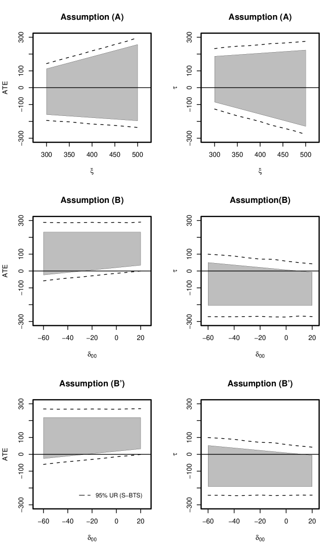
Figure 1: Sensitivities of bound estimates to $\xi=\xi_{0}=\xi_{1}$ under Assumption (A); to $\delta_{00}$ under Assumptions (B) and (B’). The gray zones show the bound estimates as a function of $\xi$ or $\delta_{00}$. The bootstrap strong 95% ${\rm UR_{S\mbox{-}BTS}}$’s are shown as dashed lines.

For (B) and (B’), we let $\delta_{00}$ (the lower limit of treatment effect among ${\mathcal{P}_{00}}$) rang from $-60$ to $20$ and fix $\delta_{11}=\delta_{y0}=\delta_{trt}=0$. (More sophisticated sensitivity analyses that jointly evaluate $\delta_{11}$, $\delta_{00}$, $\delta_{y0}$ and $\delta_{trt}$ are possible.) We choose this range for $\delta_{00}$ based on the magnitude of the AT and IPW estimates, and have it tilt toward the negative side for the possibility that HAART could be harmful for those never receiving HAART. Figure 1 (Second and third rows) shows that $\delta_{00}$ only affects the lower (upper) bound estimates of the ATE (of $\tau$). The ATE can be as high as over 200 cell/mm³, and the lower bound of ATE varies around zero depending on the value of $\delta_{00}$. Again, a possible negative value of $\tau$ suggests that unmeasured confounding likely causes HAART to be preferentially prescribed to those with poorer health.

7 Discussions

In the study of HERS, we propose to use an IV and sets of contextually plausible assumptions to quantify the causal effect of a treatment as well as the degree of unmeasured confounding. We consider three sets of assumptions. Assumption (A) specifies the limits of the expected unobservable potential outcomes, which leads to a simplified version of the Robins-Manski bounds on ATE. Assumptions (B) and (B’) specify the relative magnitudes between identified and unidentified potential outcome averages, and lead to bounds that can be much tighter than (A). The 95% uncertainty regions for the ATE under (B) and (B’) are more informative than the 95% CI of the IV estimate, and have less concern of having unmeasured confounding bias compared to the 95% CI of the IPW estimate. The bound estimates on the ATE and $\tau$ reveal that unmeasured confounding could cause a downward bias on the ATE because of HAART being preferentially prescribed to those with poorer health condition.

Quantifying the degree of unmeasured confounding can be valuable for analysis of studies conducted in similar settings but having no IV. Several HIV observational studies (e.g. Gange et al. 2007) have been conducted contemporarily as the HERS, and could suffer from similar amount of unmeasured confounding. In those studies when unmeasured confounding is of concern, analyses should be complemented with a sensitivity analyses as described in Section 6.3. A plausible range for $\tau$ can be informed from our study.

In this paper, we use the type of study site as an instrument variable, assuming that two crucial IV assumptions (monotonicity and exclusion restriction) are satisfied. The observed HAART assignment rate at academic centers is higher than that at community clinics. Such an observation suggests that the deterministic monotonicity $\Pr(A_{1}\geq A_{0})=1$ is plausible, but this assumption cannot be verified. As one limitation of our study, this assumption will be violated if some individuals would receive HAART at community clinics but not at academic medical centers. If the proportion of these individuals (${\mathcal{P}_{10}}$) is small, the bias due to the violation of the monotonicity assumption is probably negligible. Alternatively, one can assume that ${\mathcal{P}_{00}}$ is absent, so that ${\mathcal{P}_{11}}$, ${\mathcal{P}_{01}}$ and ${\mathcal{P}_{10}}$ form a partition of the population. This assumption allows everyone to have some chance of receiving HIV therapy, which is also sensible for the HERS because these patients’ CD4 counts are less than 350 six months before, and allows for the possibility that some people would potentially be treated at a community clinic but not an academic medical center. With this assumption, the proportions of ${\mathcal{P}_{11}}$, ${\mathcal{P}_{01}}$ and ${\mathcal{P}_{10}}$ are identified because $\pi_{01}=\Pr(A=0|Z=0)$, $\Pr({\mathcal{P}_{10}})=\Pr(A=0|Z=1)$, and $\Pr({\mathcal{P}_{11}})=1-\pi_{01}-\Pr({\mathcal{P}_{10}})$. The following estimands are also identified: $\mathrm{E}\{Y(0)|{\mathcal{P}_{01}}\}=\mathrm{E}(Y|A=0,Z=0)$, $\mathrm{E}\{Y(0)|{\mathcal{P}_{10}}\}=E(Y|A=0,Z=1)$, $\mathrm{E}\{Y(1)|{\mathcal{P}_{11}}\textrm{or}{\mathcal{P}_{01}}\}=\mathrm{E}(Y|A=1,Z=1)$, and $\mathrm{E}\{Y(1)|{\mathcal{P}_{11}}\textrm{or}{\mathcal{P}_{10}}\}=\mathrm{E}(Y|A=1,Z=0)$. A challenge here is how to incorporate the IV estimator, which now has an estimand as a ‘weighted’ contrast of the average treatment effects between ${\mathcal{P}_{01}}$ and ${\mathcal{P}_{10}}$, to construct constraint similar to (1). This may be worth further investigation.

Moreover, replacing the deterministic monotonicity with a stochastic monotonicity assumption deserves explorations in the future. Roy et al. (2008) assumed $\Pr(A_{1}=1|A_{0}=1,V)\geq\Pr(A_{1}=1|A_{0}=0,V)$, and proposed to use auxiliary covariates to estimate the memberships of principal strata. Small and Tan (2008) assumed $\Pr(A_{1}=1|U)\geq\Pr(A_{0}=1|U)$ with $U$ being a latent variable satisfying certain conditions. These stochastic monotonicity assumptions allow the possible presence of ${\mathcal{P}_{10}}$ and may be more realistic in the HERS than the deterministic monotonicity.

The exclusion restriction could also be violated if the type of study site $Z$ remains associated with the outcome $Y$ after accounting for the effect of $Z$ on HAART receipt. A weaker exclusion restriction assumption can be made, if the association between the instrument and the outcome can be removed after conditioning on some measured covariate $V^{*}$, i.e. $\{Y(1),Y(0)\}\perp Z|V^{*}$. In this case, the methods by Tan (2006) can be implemented for identifying the LATE, and our method for bound estimation on ATE and $\tau$ still applies.

There are several ways to account for the measured confounding. We use the method of inverse probability weighting by specifying a propensity score model. Alternatively, we can specify both an outcome regression model and a propensity score model and use the doubly robust (DR) estimator (Bang and Robins 2005) to estimate the ATE. We do not implement the DR estimator in this paper because when unmeasured confounding exists the DR estimator is no longer guaranteed to be consistent for ATE and could suffer more bias than other estimators. The simulations of Kang and Schafer (2007) suggest that IPW is relatively robust to the impact of unmeasured confounding in term of estimation bias. Because the focus issue of this paper is unmeasured confounding, we use the IPW for estimating ATE.

References

- Angrist and Imbens [1995] Joshua D. Angrist and Guido W. Imbens. Two-stage least squares estimation of average causal effects in models with variable treatment intensity. Journal of the American Statistical Association, 90(430):431–442, 1995.
- Angrist et al. [1996] Joshua D. Angrist, Guido W. Imbens, and Donald B. Rubin. Identification of causal effects using instrumental variables. Journal of the American Statistical Association, 91(434):444–455, 1996. ISSN 0162-1459.
- Bang and Robins [2005] Heejung Bang and James M. Robins. Doubly robust estimation in missing data and causal inference models. Biometrics, 61:962–972, 2005.
- Bickel and Freeman [1981] P. J. Bickel and D. A. Freeman. Some asymptotic theory for the bootstrap. The Annals of Statistics, 9:1196–1217, 1981.
- Brumback et al. [2004] Bagette A. Brumback, Miguel A. Hernán, Sebastien J. P. A. Haneuse, and James M. Robins. Sensitivity analyses for unmeasured confounding assuming a marginal structural model for repeated measures. Statistics in Medicine, 23(5):749–767, 2004.
- Carpenter et al. [2000] C.C.J. Carpenter, D.A. Cooper, J.M. Fischl, J.M. Gatell, B.G. Gazzard, S.M. Hammer, M.S. Hirsch, D.M. Jacobsen, D.A. Katzenstein, J.S.G. Montaner, D.D. Richman, M.S. Saag, M. Schechter, M. Schooley, M. A. Thompson, S. Vella, P.G. Yeni, and P. A. Volberding. Antiretroviral therapy in adults:updated recommendations of the international aids society-usa panel. Journal American Medical Association, 283:381–391, 2000.
- Cheng and Small [2006] Jing Cheng and Dylan S. Small. Bounds on causal effects in three-arm trials with non-compliance. Journal of the Royal Statistical Society, Series B: Statistical Methodology, 68(5):815–836, 2006.
- D’Agostino [1998] R.B. D’Agostino. Tutorial in biostatistics: propensity score methods for bias reduction in the comparison of a treatment to a non-randomized control group. Statistics in Medicine, 17(19):2265–2281, 1998.
- Frangakis and Rubin [2002] Constantine E. Frangakis and Donald B. Rubin. Principal stratification in causal inference. Biometrics, 58(1):21–29, 2002.
- Gange et al. [2007] Stephen J Gange, Mari M Kitahata, Michael S Saag, David R Bangsberg, Ronald J Bosch, John T Brooks, Liviana Calzavara, Steven G Deeks, Joseph J Eron, Kelly A Gebo, M John Gill, David W Haas, Robert S Hogg, Michael A Horberg, Lisa P Jacobson, Amy C Justice, Gregory D Kirk, Marina B Klein, Jeffrey N Martin, Rosemary G McKaig, Benigno Rodriguez, Sean B Rourke, Timothy R Sterling, Aimee M Freeman, and Richard D Moore. Cohort profile: The North American AIDS cohort collaboration on research and design (NA-ACCORD). International Journal of Epidemiology, 36:294–301, 2007.
- Hernan and Robins [2006] Miguel Angel Hernan and J. M. Robins. Instruments for causal inference: An epidemiologist’s dream? Epidemiology, 17:360–372, 2006.
- Hogan and Lancaster [2004] Joseph W. Hogan and Tony Lancaster. Instrumental variables and inverse probability weighting for causal inference from longitudinal observational studies. Statistical Methods in Medical Research, 13:17–48, 2004.
- Horowitz and Manski [2000] Joel L. Horowitz and Charles F. Manski. Nonparametric analysis of randomized experiments with missing covariate and outcome data. Journal of the American Statistical Association, 95(449):77–84, 2000.
- Imbens and Angrist [1994] Guido W. Imbens and Joshua D. Angrist. Identification and estimation of local average treatment effects. Econometrica, 62(2):467–475, 1994. ISSN 0012-9682.
- Joffe [2001] Marshall M. Joffe. Using information on realized effects to determine prospective causal effects. Journal of the Royal Statistical Society. Series B: Statistical Methodology, 63(4):759–774, 2001. ISSN 1369-7412.
- Kang and Schafer [2007] J. D. Y. Kang and J. L. Schafer. Demystifying double robustness: A comparison of alternative strategies for estimating a population mean from incomplete data. Statistical Science, 22:523–539, 2007.
- Ko et al. [2003] Hyejin Ko, Joseph W. Hogan, and Kenneth H. Mayer. Estimating causal treatment effects from longitudinal HIV natural history studies using marginal structural models. Biometrics, 59:152–162, 2003.
- Manski [1990] C.F. Manski. Nonparametric bounds on treatment effects. American Economic Reviews, Papers and Proceedings, 80:319–323, 1990.
- Miguel et al. [2001] Hernan A Miguel, Brumback Babette, and J. M. Robins. Marginal structural models to estimate the joint causal effect of nonrandomized treatments. Journal of the American Statistical Association, 96:440–448, 2001.
- Robins [1989] J. M. Robins. The analysis of randomized and nonrandomized AIDS treatment trials using a new approach to causal inference in longitudinal studies, chapter Health Service Research Methodology: A Focus on AIDS, pages 213–290. Washington D.C.: U.S. Public Health Service, 1989.
- Robins [1999] James M. Robins. Association, causation, and marginal structural models. Synthese, 121:151–179, 1999.
- Robins et al. [1994] James M. Robins, Andrea Rotnitzky, and Lue Ping Zhao. Estimation of regression coefficients when some regressors are not always observed. Journal of the American Statistical Association, 89(427):846–866, 1994. ISSN 0162-1459.
- Robins et al. [2000] James M. Robins, Miguel Ángel Hernán, and Babette Brumback. Marginal structural models and causal inference in epidemiology. Epidemiology, 11:550–560, 2000.
- Robins et al. [1999] J.M. Robins, A. Rotnitzky, and D.O. Scharfstein. Sensitivity analysis for selection bias and unmeasured confounding in missing data and causal inference models. Statistical Models in Epidemiology: The Environment and Clinical Trials, 116:1–92, 1999.
- Rosenbaum and Rubin [1983] Paul R. Rosenbaum and Donald B. Rubin. The central role of the propensity score in observational studies for causal effects. Biometrika, 70(1):41–55, 1983.
- Rosenbaum [2002] P.R. Rosenbaum. Observational studies. Springer, 2002.
- Rosenbaum and Rubin [1984] P.R. Rosenbaum and D.B. Rubin. Reducing bias in observational studies using subclassification on the propensity score. Journal of the American Statistical Association, 79(387):516–524, 1984.
- Roy et al. [2008] Jason Roy, Joseph W. Hogan, and Bess H. Marcus. Principal stratification with predictors of compliance for randomized trials with 2 active treatments. Biostatistics, 9:277–289, 2008.
- Rubin [1974] D. B. Rubin. Estimating causal effects of treatments in randomized and nonrandomized studies. Journal of Educational Psychology, 66:668–701, 1974.
- Small and Tan [2008] Dylan S. Small and Zhiqiang Tan. A stochastic monotonicity assumption for the instrumental variables method. Technical report, University of Pennsylvnia, 2008.
- Smith et al. [1997] D.K. Smith, D. Warren, P. Vlahov, P. Schuman, M.D. Stein, B.L. Greenberg, and S.D. Holmberg. Design and baseline participant characteristics of the human immunodeficiency virus epidemiology research (HER) study: a prosepective cohort study of human immunodeficiency virus infection in us women. American Journal of Epidemiology, 146:459–469, 1997.
- Stock and Trebbi [2003] J.H. Stock and F. Trebbi. Retrospectives: Who invented instrumental variable regression? The Journal of Economic Perspectives, 17(3):177–194, 2003.
- Tan [2006] Zhiqiang Tan. Regression and weighting methods for causal inference using instrumental variables. Journal of the American Statistical Association, 101(476):1607–1618, 2006.
- Ten Have et al. [2008] T.R. Ten Have, S.L.T. Normand, S.M. Marcus, C.H. Brown, P. Lavori, and N. Duan. Intent-to-treat vs. non-intent-to-treat analyses under treatment non-adherence in mental health randomized trials. Psychiatric annals, 38(12):772, 2008.
- VanderWeele and Shpitser [2011] T.J. VanderWeele and I. Shpitser. On the definition of a confounder. Technical report, bepress, 2011.
- Vansteelandt et al. [2006] Stijn Vansteelandt, Els Goetghebeurand, Michael G. Kenward, and Geert Molenberghs. Ignorance and uncerntainty regions as inferential tools in a sensitivity analysis. Statistica Sinica, 16:953–979, 2006.
- Wooldrige [2002] Jefferey M. Wooldrige. Econometric Analysis of Cross Section and Panel Data. Cambridge, MA: MIT Press., 2002.
- Wright [1928] S Wright. Appendix to the Tariff on Animal and Vegetable Oils, by P. G. Wright,, volume 26. New York: MacMillan., 1928.
- Zhang and Rubin [2003] J. L. Zhang and D. B. Rubin. Estimation of causal effects via principal stratification when some outcomes are truncated by death. Journal of Educational and Behavioral Statistics, 28:353–368, 2003.