Multiphoton Ionization of Magnesium in a Ti-Sapphire laser field

Abstract

In this paper we report the theoretical results obtained for partial ionization yields and the above-threshold ionization (ATI) spectra of Magnesium in a Ti:sapphire laser field (804 nm) in the range of short pulse duration (20-120 fs). Ionization yield, with linearly polarized light for a 120 fs laser pulse, is obtained as a function of the peak intensity motivated by recent experimental data gillen:2001 . For this, we have solved the time-dependent Schrödinger equation nonperturbatively on a basis of discretized states obtained with two different methods; one with the two-electron wavefunction relaxed at the boundaries, giving a quadratic discretized basis and the other with the two-electron wavefunction expanded in terms of Mg⁺-orbitals plus one free electron allowing the handling of multiple continua (open channels). Results, obtained with the two methods, are compared and advantages and disadvantages of the open-channel method are discussed.

1 Introduction

Experimental studies of above threshold ionization have concentrated mostly on the rare gases pet ; scf ; nan ; buc which can withstand sufficiently large intensities of radiation of wavelength around 780 to 800 nm, which is the most versatile and convenient source of short pulse duration. As a result, extensive studies of ATI photoelectron spectra, and of course high order harmonics, in the non-perturbative regime have and are being conducted bur ; corm ; jian:1995a ; jian:1996 . Softer atoms, with lower ionization potentials are not expected to exhibit the extensive spectra of ATI, as they ionize at relatively lower intensities. Nevertheless, recent experimental studies gillen:2001 ; druten:1994 have addressed this issue in atomic Magnesium, which not only is a soft atom but also has two valence electrons, which may or may not add additional features, depending on intensity and pulse duration. The results have been rather surprising. The slopes of the ATI spectra as a function of laser intensity are difficult to understand gillen:2001 . This motivated the theoretical study whose main results are presented in this paper. The study was undertaken because we happened to have developed the theoretical tools necessary for a realistic description of Magnesium as a correlated two-electron system. Although under the conditions of the experiment gillen:2001 , it does not appear that two-electron excitations played an important role, at least in the aspects we have addressed, still we can say that the atomic structure entering the calculation is realistic. We have not calculated everything that has been measured experimentally. We present our results as a point of calibration of what can be expected theoretically. As discussed in the sections that follow, we find it difficult to understand the observed slopes. If it is because something is missing in our calculation, at this point we are unable to say what it could be.

2 Two-electron continuum states of Magnesium

The Hamiltonian of the Magnesium atom $H_{a}$ can be written as:

$$H_{a}=\sum_{i=1}^{2}\left[-\frac{1}{2}\nabla_{i}^{2}+V_{eff}(\mathbf{r}_{i})\right]+V(\mathbf{r}_{1},\mathbf{r}_{2}),$$ (1)

where $V_{eff}(\mathbf{r}_{i})$ represents the effective potential for the $i^{th}$ electron and the core, and $V(\mathbf{r}_{1},\mathbf{r}_{2})$ is a two-body interaction operator, that includes the static Coulomb interaction $1/|{\bf r}_{1}-{\bf r}_{2}|$ as well as a dielectronic effective interaction chang:1993a ; moccia:1996a .

The characteristic feature of Magnesium is the existence of an $ns^{2}$ valence shell, outside a closed-shell core, the excitation of which requires a much larger amount of energy compared with the first and second ionization threshold. This allows us to explore excitation and/or ionization processes of the valence electrons, without considering the closed-shell core-excitation, for a certain range of photon energies. The construction of the Magnesium bound and final states is achieved through a standard Hartree-Fock calculation and the inclusion of a core-polarization potential which represents the influence of the core on the two valence electrons in a way very similar to that described in chang:1993a ; nikolopoulos:2002a .

At a first stage, we perform a Hartree-Fock calculation for the closed-shell core of Magnesium (Mg⁺⁺), deriving thus the effective Hartree-Fock potentials ’seen’ by an outer electron. At a second stage, we solve the Schrödinger equation for Mg⁺. In this case, the effective potential acting on the valence electron is given by moccia:1996a ,

$$V_{eff}(r)=V_{l}^{HF}(r)+\frac{\alpha_{s}}{r^{4}}\left[1-e^{-(\frac{r}{r_{l}})^{6}}\right],$$ (2)

where $\alpha_{s}$ is the static polarizability of the doubly-ionized Mg and $r_{l}$ cut-off radii for the various partial waves $l=0,1,2,...$ .

Having produced the Mg⁺ one-electron radial eigenstates $P_{nl}(r)$ for each partial wave $l=0,1,2,...$, we solve the Schrödinger equation:

$$H_{a}\Psi^{\Lambda}({\bf r}_{1},{\bf r}_{2})=E\Psi^{\Lambda}({\bf r}_{1},{\bf r}_{2}),$$ (3)

by expanding the two-electron eigenstates $\Psi^{\Lambda}({\bf r}_{1},{\bf r}_{2})$ on the basis of two-electron antisymmetrized orbitals namely:

$$\Psi^{\Lambda}({\bf r}_{1},{\bf r}_{2};E_{i})=\sum_{nll^{\prime},n^{\prime}}C_{nll^{\prime}n^{\prime}}(E_{i})\Phi_{nln^{\prime}l^{\prime}}^{\Lambda}({\bf r}_{1},{\bf r}_{2})$$ (4)

$$\Phi^{\Lambda}_{nln^{\prime}l^{\prime}}({\bf r}_{1,}{\bf r}_{2}) = A_{12}\frac{P_{nl}(r_{1})}{r_{1}}\frac{R_{n^{\prime}l^{\prime}}(r_{2})}{r_{2}}$$ (5)

$$\times Y_{LM_{L}}(\hat{r}_{1},\hat{r}_{2};l,l^{\prime})Y_{S,M_{S}}(s,s^{\prime}),$$

where $A_{12}$ is the antisymmetrization operator which ensures that the total wave function, is anti-symmetric with respect to interchange of the space and spin coordinates of the two electrons. $\Lambda$ represents the set of angular quantum numbers $(LSM_{L}M_{S})$. In Eq.(5) the choice of the basis functions $R_{nl}(r)$ determines the method used for the calculation of the correlated two-electron states.

In the case of fixed boundary conditions (FXBC), we force the wavefunction to be zero at the boundaries by selecting the basis functions $R_{nl}(r)$ to be the one-electron radial solutions of Mg⁺, which by construction vanish at the boundaries. This, transforms the Schrödinger Eq.(3) into a generalized eigenvalue matrix equation, by the diagonalization of which we obtain the coefficients $C_{nll^{\prime}n^{\prime}}(E_{i})$ for each discrete eigenvalue $E_{i}$ chang:1993b ; lambropoulos:1998 ; nikolopoulos:2002a . This choice of the basis functions $R_{nl}(r)$ leads thus to a discretized continuum spectrum for the Magnesium atom with density of states determined basically from the box radius $R$.

On the other hand, we can select the basis function $R_{nl}(r)$ to be non-vanishing at the boundaries (FRBC) transforming the Schrödinger Eq.(3) into a system of algebraic equations for the coefficients $C_{nll^{\prime}n^{\prime}}(E_{i})$ lambropoulos:1998 ; nikolopoulos:2001a . For this, we use for both cases (FXBC and FRBC) the B-spline basis functions deboor:1978 used extensively in the last 15 years in atomic structure calculations. The main advantage of this method over the FXBC method is that the density of the continuum spectrum is completely controllable (therefore degeneracy into the continuum is guaranteed) and the two-electron continuum states have been expanded in terms of core-target states plus an ionized electron, as in standard close-coupling scattering theory.

We have ascertained that the results obtained with the free boundary method compare well with the convergent results obtained with the fixed boundary method.

3 Time-dependent Schrödinger Equation

Our objective is to solve the time-dependent Schrödinger equation (TDSE) :

$$\frac{d}{dt}\Psi({\bf r}_{1},{\bf r}_{2};t)=-i\left[H_{a}+V(t)\right]\Psi({\bf r}_{1},{\bf r}_{2};t).$$ (6)

The time-dependent interaction $V(t)$ of the two-valence electron atom with an external laser pulse in the dipole approximation and velocity gauge can be written as:

$$V(t)=-A(t)\hat{\varepsilon}\cdot({\bf p}_{1}+{\bf p}_{2}),$$ (7)

where the vector potential $A(t)$ is given by,

$$A(t)=A_{0}f(t)\cos(\omega t),$$ (8)

${\hat{\varepsilon}}$ is the unit polarization vector of the laser field, and ${\bf p}_{1,2}$ are the momenta of the two valence electrons. $A_{0}=E_{0}/\omega$ is the amplitude of the vector potential, and ${\textrm{E}}_{0}$ the electric field strength. The pulse shape envelope is $f(t)=\cos^{2}\left({\pi t}/{\tau}\right)$, where $\tau$ is approximately the full width at half maximum (FWHM) for the electric field. The integration time for the cosine squared shape pulse, is taken from $-\tau/2$ to $\tau/2$. The velocity form of the interaction Hamiltonian is chosen, because it makes the calculation converge faster, in terms of the number of angular momenta included cormier:1996a . It should be noted here that length and velocity dipole matrix elements agree very well. For the length operator, for the reason that the core-polarization potential is angular momentum dependent, we have checked that the use of the modified operator as given by mitroy:1988 , ${\bf r}^{\prime}={\bf r}-{\bf\hat{r}}(\alpha_{s}/r^{2})[1-e^{-(r/r_{l})^{6}}]$ has very small effect in the dipole matrix elements compared with those calculated with the standard length operator.

The time-dependent wavefunction is now expanded on the basis of eigenfunctions $\Psi^{\Lambda}({\bf r}_{1},{\bf r}_{2};E_{i})$,

$$\Psi({\bf r}_{1},{\bf r}_{2};t)=\sum_{E_{i},L}U_{L}(E_{i},t)\Psi^{\Lambda}({\bf r}_{1},{\bf r}_{2};E_{i}),$$ (9)

transforming the time-dependent Schrödinger equation into a set of first-order differential equations for the time-dependent coefficients $U_{L}(E_{i},t)$, namely,

$$i\frac{d}{dt}U_{L}(E_{i},t)=\sum_{E_{i^{\prime}}L^{\prime}}[E_{i,L}\delta_{ii^{\prime}}\delta_{LL^{\prime}}-V_{E_{i}L,E_{i^{\prime}}L^{\prime}}(t)]U_{L^{\prime}}(E_{i^{\prime}},t)$$ (10)

subject to the initial conditions $|U_{L}(E_{i},t=0)|^{2}=\delta_{E_{i}E_{1}}\delta_{L0}$. The quantities $V_{E_{i}L,E_{i^{\prime}}L^{\prime}}(t)$ represent the matrix elements of $V(t)$ calculated between the states characterized by the quantum numbers $E_{i}L$ and $E_{i^{\prime}}L^{\prime}$. Assuming that the laser field is linearly polarized, and the Magnesium atom initially in its ground state $(L=0,l_{1}=l_{2}=0,M=0)$, we need to consider only the $M=0$ singlet states ($S=0$).

At the end of the pulse, we obtain the coefficients $U_{L}(E_{i},t\rightarrow\infty)$, from which we can extract information about the ionization yields, photoelectron energy spectrum as well as photoelectron angular distributions lambropoulos:1998 ; nikolopoulos:1999 .

4 Results and discussion

Compared to the Helium atom, the Magnesium continua associated with more than one ionization threshold lie much closer to the lowest one (one open channel) which makes them much more accessible at intensities, frequencies, and pulse durations currently available. That is why excited ionic states have often been observed in alkaline earth atoms.

For laser intensities of about $I_{0}<10^{12}$ W/cm² of a Ti:sapphire laser at 804 nm (1.54 eV), five photons are required to ionize the Magnesium atom

$${\rm Mg}(3s^{2})+5\omega\rightarrow{\rm Mg}^{+}(3s)+e^{-}(0.06\;{\rm eV}),$$ (11)

and leave the Mg⁺ in its ground state, as illustrated in the energy-level diagram in Figure 1. At higher intensities as the ponderomotive shift increases, at least six photons are required to ionize the Magnesium atom and the $3s3p$ state can be reached through a three-photon absorption. If we consider, for example, 11-photon ionization in Magnesium, five of the photons will bring the atom in the ground ionic state plus one electron in the associated continuum, and the remaining ones will be absorbed with the possibility to excite further the ionized electron (above-threshold ionization) and/or to excite the core to different ionic states. The calculation of the probability of this channeling into the final ionization stages of the Magnesium, after the interaction with the laser, is a difficult task. In the following paragraphs, we discuss the results obtained with two different methods each having its own advantages and disadvantages.

Populating the first excited ionic state ${\textrm{Mg}}^{+}(3p)$ is possible by the absorption of eight photons. With the absorption of an additional three photons, the ionic excited states ${\textrm{Mg}}^{+}(4s)$ and ${\textrm{Mg}}^{+}(3d)$ become also energetically accessible. The position in energy of the ionic thresholds in Figure 1, is for the bare atom without taking into account the shift of the energy levels in the laser field. In the presence of an intense laser, the ionization threshold of an atom is increased by the ponderomotive energy. If the intensity of the laser is sufficiently high, channel closing will occur so that $N\hbar\omega<I_{p}+U_{p}$, where $I_{p}=-E_{a}$ is the ionization potential corresponding to the energy of the ionization threshold $E_{a}$, $N$ is the number of photons required to ionize the atom, and $U_{p}$ is the ponderomotive energy which is given in atomic units by $U_{p}={\textrm{E}}_{0}^{2}/4\omega^{2}$. In the case of photon energy $\omega=1.54$ eV the ponderomotive shift is $U_{p}\simeq$ 0.6 eV at the intensity $I$=10¹³ W/cm².

A related phenomenon which occurs in strong laser fields is that large AC-Stark shifts in atomic states can lead to intermediate resonances in the ionization process agostini:1989 . At intensities around $2.4\times 10^{12}$ W/cm², the excited state of the Magnesium atom $3s3p$ is shifted into resonance.

4.1 Fixed boundary condition method

We have studied the intensity dependence of both ion yield and the photoelectron spectrum of Magnesium in the Ti-Sapphire laser field in the domain of short pulse duration for laser intensities up to $10^{14}$ W/cm² with two-electron states of Magnesium calculated with the fixed boundary method. The results presented are converged in terms of box size, number of B-splines and angular momenta.

In Figure 2, we show the yield of Magnesium ions as a function of the laser intensity, for photon energies $\omega=1.54$ eV, and laser pulse duration $\tau=35$ optical cycles ($\sim 93$ fs) and $\tau=45$ optical cycles ($\sim 120$ fs). We have employed a basis of $992$ B-splines in a box of $1900$ a.u, and a total number of angular momenta up to L = 9.

According to perturbation theory, the $N$-photon generalized cross section is proportional to the $N^{th}$ power of the photon flux. Therefore the slope of the ionization yield versus laser intensity in a logarithmic scale represents the minimum number of photons necessary to ionize the atom. Since the Magnesium states in the continuum are shifted in the laser field with the ponderomotive potential, at least six photons must be absorbed to ionize the Magnesium atom for laser intensities higher than $10^{12}$ W/cm².

For intensities in the range between $10^{12}$ W/cm² and $10^{13}$ W/cm², and for both the 93 and 120 fs pulses we found slopes for the ionization yield curves around 6 which are basically in agreement with the lowest-order perturbation theory (LOPT) predictions. The ionization yield of Mg⁺ increases linearly with the peak intensity of the field until the saturation regime is reached, where a decrease in the slope begins. Around $10^{13}$ W/cm², however, we have found a sudden enhancement of the ionization yield which is attributed to AC-stark shifting of the Rydberg states into resonance with the laser field. Though this enhancement is apparent in our results, the slope does not compare to that (of about $11$) reported in the recent experiment by gillen:2001 , in the same range of intensities.

In Figure 3 we have plotted the ground state population, the ionization yield as well as the population of states $3s3p$ and $3s4f$. In this figure one can see that at peak intensity of about $1.3\times 10^{13}$ W/cm² the ionization yield makes an abrupt ’jump’. At the same intensity the population of the state $3s4f$ is almost 10$\%$ of the ionization yield (almost equal with the remaining population in the ground state) while the population of the $3s3p$ state becomes negligible. In Figure 4 we have plotted for the peak intensity $1.3\times 10^{13}$ W/cm² the populations of the same states as in Figure 3 and the ionization yield during as a function of the time. The $3s3p$ state is populated during the rise of the pulse while at the end of the pulse the population of the $3s3p$ state has been ’transferred’ to the $3s4f$ state, which becomes the dominant, in population, excited state.

4.2 Free boundary condition method

We produce the initial ground state of Magnesium in a box of radius $R=40$ a.u. in which we have included only 20 configuration series of the type $nsms,npmp,ndmd,nfmf$ with $n,m$ up to 5. The number of B-splines basis was 62 and the order 9. The parameters of the core-polarization potential included in Eq.2 were $\alpha_{s}=0.491$ for the static polarizability of the closed-shell core and 1.2, 1.335, 1.25, 1.3, 1.1 for the cut-off radii for the $l=0,1,2,3,4,$ partial waves, respectively. This resulted to a value for the singly ionized Magnesium equal $E$(Mg${}^{+}(3s))=-14.99$ eV and a value for the Magnesium ground state equal to $-22.653$ eV measured from the double ionization threshold. The energy value for the intermediate $3s3p$ state was $-18.32$ eV.

The basis used for the propagation of the TDSE differs from the one used in the FXBC case in two aspects: firstly, we have produced our basis in a much smaller box (of radius 40 a.u) than that of the FXBC basis ($\sim 600\div 2000$ a.u.) which results in the absence of high Rydberg states in the Mg bound spectrum. Thus, while in the FXBC basis a number of Rydberg states of about $\sim 30\div 40$ might be obtained, depending on the value of the box radius, in the FRBC basis a number of 5 Rydberg states is obtained. Moreover, we have calculated a total number of angular momenta, up to five. The only reason for this restriction of the FRBC basis is computational resources limit. It is the price that one has to pay in going from the FXBC method to the FRBC method. The expansion of the two-electron states in a set of target - core states plus one free electron, allows us to obtain much more detailed information for the states of the atom after its interaction with the laser, such as partial ionization yields (populations of the various ionization stages of the ionized system), partial photoelectron spectra (branching ratios) and moreover angular photoelectron distributions. Thus it is expected, that quantitative differences are to be found between the two approaches due to the limited basis used in the FRBC approach. It is absolutely necessary, therefore, that one should ensure that results calculated with both methods are in good agreement, since in an unlimited basis case they have to be the same.

With this in mind, we have compared in Figure 5 the ionization yield in Magnesium calculated with the free boundary method for a pulse duration of about 29.5 fs (full curve) with the ionization yield calculated with the fixed boundary method of about 27 fs (dotted curve). We have employed a basis of $802$ B-splines in a box of $900$ a.u and calculated two-electron states with total angular momenta up to L = 9, for the results obtained with the fixed boundary method. For short pulse duration, the agreement between these two methods is rather good. The corresponding slope of the ionization yields is 4.46 and 4.25 for the FXBC and FRBC method, respectively. Similar agreement is obtained for the photoelectron energy spectrum for the pulses employed here, though not presented.

In Figure 6, we have plotted the ion yield versus intensity of the laser field, of Magnesium ions left in different states, for photon energy $\omega=1.54$ eV and 93 fs pulse duration, calculated with a cosine squared pulse. From the ionization yield curves, we found that the Mg ion is preferentially left in the $3s$ ground state in the intensity domain smaller than $2\times 10^{13}$ W/cm². The slope of the corresponding curve (represented by the dotted line) has the value 5.96 around the peak intensity $I_{0}=10^{12}$W/cm². We should mention here the difference in the slope of the ionization yield between the shorter pulse (fig. 5) which gives a slope of about $\sim 4.4$. For the longer pulse the photon energy spectrum of the field is much less broader than in the case of the shorter pulse. Due to bandwidth of the shorter pulse, a three photon absorption from the ground state populates strongly the 3s3p excited state which for that reason, plays the role of an intermediate resonance thus lowering the order of the slope of the ionization yield, as expected from energy conservation rules, according LOPT predictions. Note that, ionization from the 3s3p state requires the absorption of three more 1.55 eV photons. Similar role plays the ionization threshold at about $\sim 7.64$ eV, while the 5-photon (1.55 eV) absorption brings the system in an energy very close to the ionization threshold.

In the presence of resonances, the ionization rate for multiphoton processes measured as a function of intensity will deviate from the power-law $I^{N}$ dependence lambropoulos:1976 . Since we are dealing with near resonant multiphoton ionization with the $3s3p$ state of Magnesium, the slopes of the ionization yields for the Mg${}^{+}(3p)$, Mg${}^{+}(4s)$, and Mg${}^{+}(3d)$ thresholds are smaller than those predicted by perturbation theory. In order to have a better picture of the amount of ions left in different excited states, we have calculated the branching ratios in photoelectron spectra corresponding to different ionization channels and their dependence on laser intensity. In Figure 7, we have plotted the branching ratios of partial ionization yields, namely the number of ions left in a particular state of the Magnesium ion (ground or excited). The branching ratios have been calculated by integrating over the energy the partial photoelectron spectrum associated with that state. It is well-known that, within lowest-order perturbation theory, the branching ratios are independent of laser intensity, as we can observe at intensities less than $2\times 10^{12}$ W/cm² for $3p$ and $4s$ ionization thresholds. At moderate intensities, the number of ions left in Mg${}^{+}(3p)$ state, represented by the dotted curve, is greater than the ions left in the Mg${}^{+}(3d)$ state (dot-dashed curve) and Mg${}^{+}(4s)$ state (dashed curve). For higher intensities, in the saturation domain, the amount of ions left in the Mg${}^{+}(3p)$ and Mg${}^{+}(3d)$ excited states are of comparable value.

We also present in Figure 8, the partial photoelectron energy spectra corresponding to ions left in the ground state (full curve) and in different excited states: $3p$ (dotted curve), $3d$ (dashed curve), $4s$ (dot-dashed curve) calculated for a peak intensity of the laser pulse $2\times 10^{12}$ W/cm². The spectrum associated with the $3p$ threshold is hidden under the dominant contribution associated with the $3s$ threshold. This overlap can be attributed to the fact that the $3s$ and $3p$ thresholds are about $4.44$ eV apart, so that the first photoelectron peak above the $3s$ threshold has only $0.18$ eV energy less than the first peak above the $3p$ threshold.

5 Conclusion

In conclusion, we have calculated ionization yields and ATI spectra of Magnesium subject to a pulse of duration of 93 fs and 120 fs for the Ti:sapphire laser (804 nm) for the range of intensities between 10¹² W/cm² and 5$\times$ 10¹³ W/cm². For this, we have employed a well established method, based on a configuration interaction discretized two-electron states, developed over the last few years jian:1995a ; jian:1996 ; nikolopoulos:1999 ; tang:1990 ; tang:1991 , and in addition we have presented an alternative method to solve nonpertubartively the time-dependent Schrödinger equation that handles ionization stages of two-electrons atoms with multiple continua (many open channels). Partial ionization yields, photoelectron spectra and photoelectron angular distributions (though not presented in this work) may be obtained with this open-channel method.

As already mentioned in the text, the slopes of the ion yield as a function of laser intensity that we obtain are considerably lower than those observed by Gillen et al gillen:2001 . Our calculations have not included averaging over the interaction volume. Such averaging in any case tends to lower rather than increase the slopes of the ion yield curves. The effect of resonance with intermediate atomic states is inherent in our calculations. But in any case, it is not expected to raise slopes. Thus at this point, we have no clue as to the possible reasons for the discrepancy. Hopefully, further experimental and possibly theoretical work will shed some light on this puzzle.

TABLE - FIGURE CAPTIONS

FIG. 1. Energy-level diagram for Magnesium showing the levels relevant for this study. The energies are referenced with respect to the neutral Magnesium ground state.

FIG. 2. Ionization yield in Magnesium as a function of peak laser intensity for photon energies $\omega=1.54$ eV. Pulse duration is 93 fs (35 optical cycles) and 120 fs (45 optical cycles).

FIG. 3. Population of $3s^{2},3s3p,3s4f$ states and ionization yield (Y), at the end of the pulse, as a function of the peak laser intensity, for the 93 fs pulse.

FIG. 4. Population of $3s^{2},3s3p,3s4f$ states and ionization yield (Y) as a function of the interaction time, for the 93 fs pulse, and peak intensity $1.3\times 10^{13}$W/cm².

FIG. 5. Comparison of ionization yields in Magnesium calculated with FRBC method (full curve) and FXBC (dotted curve) method as a function of the peak laser intensity for photon energy at 804 nm (1.54 eV).

FIG. 6. Ionization yield in Magnesium as a function of peak laser intensity for photon energies $\omega=1.54$ eV. Pulse duration is 93 fs (35 optical cycles).

FIG. 7. Branching ratios of Mg⁺ ions left in different excited states as a function of laser intensity. The parameters are the same as in Figure 6.

FIG. 8. Photoelectron ATI energy spectra corresponding to Mg⁺ left in the ground state as well as a few excited states. The laser peak intensity is $I_{0}=2\times 10^{12}$ W/cm², the rest of the parameters are the same as in Figure 6.

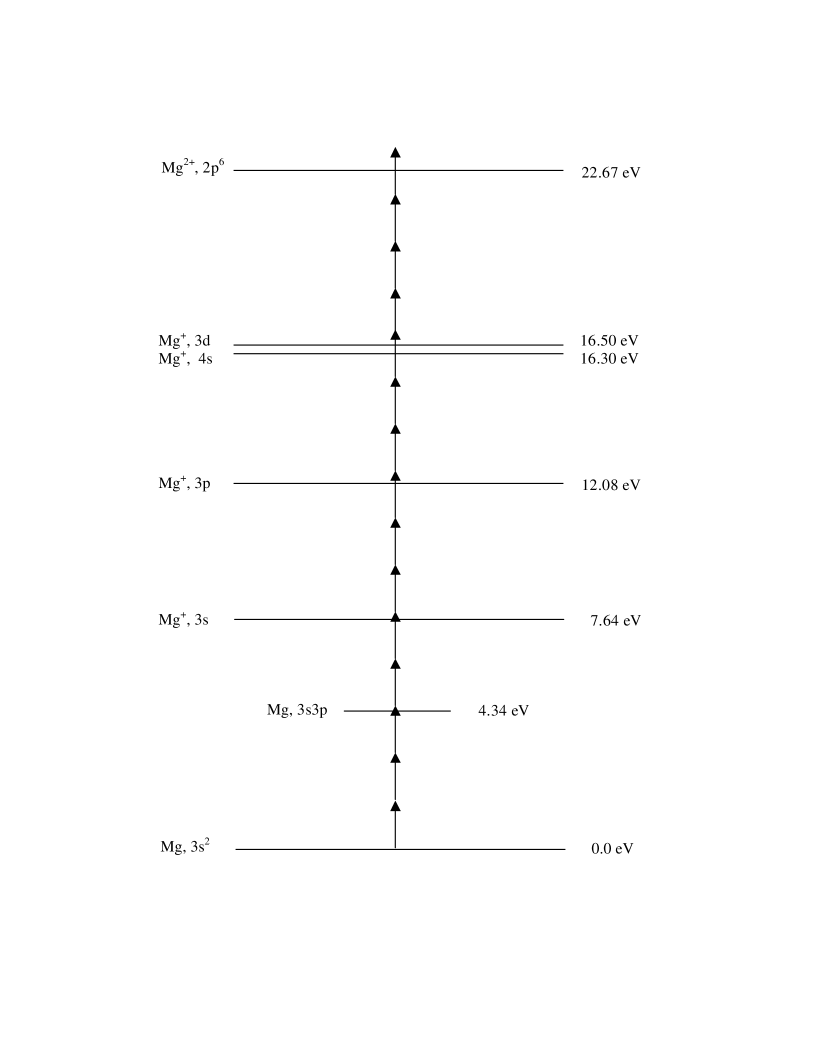
Figure 1:

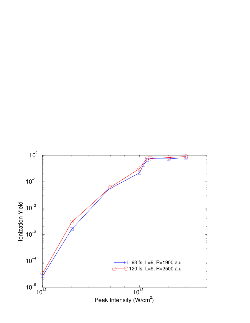
Figure 2:

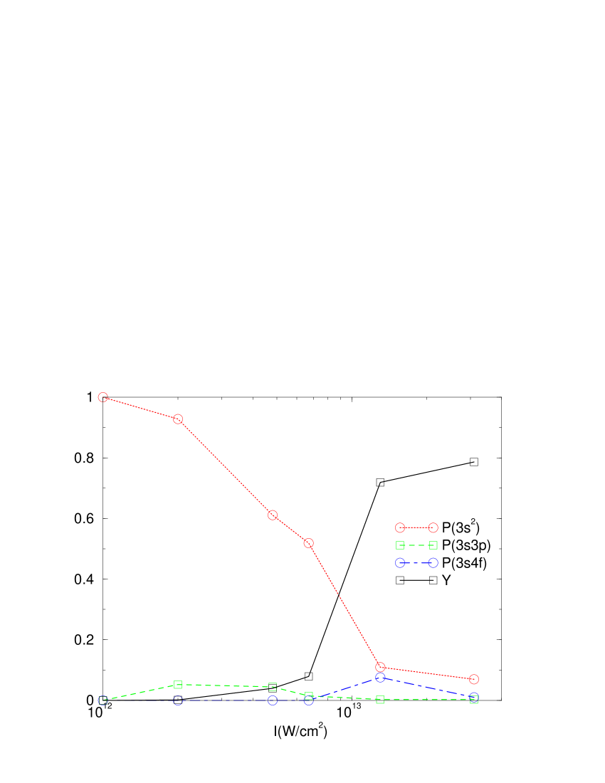
Figure 3:

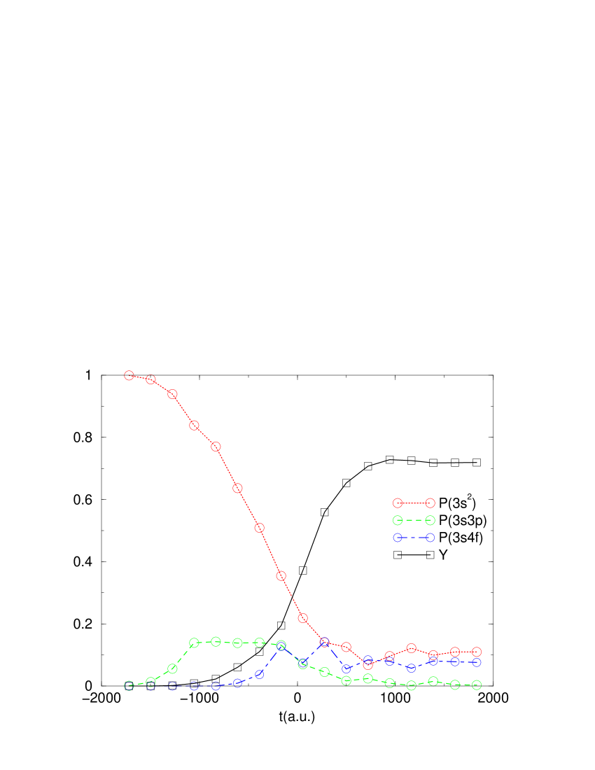
Figure 4:

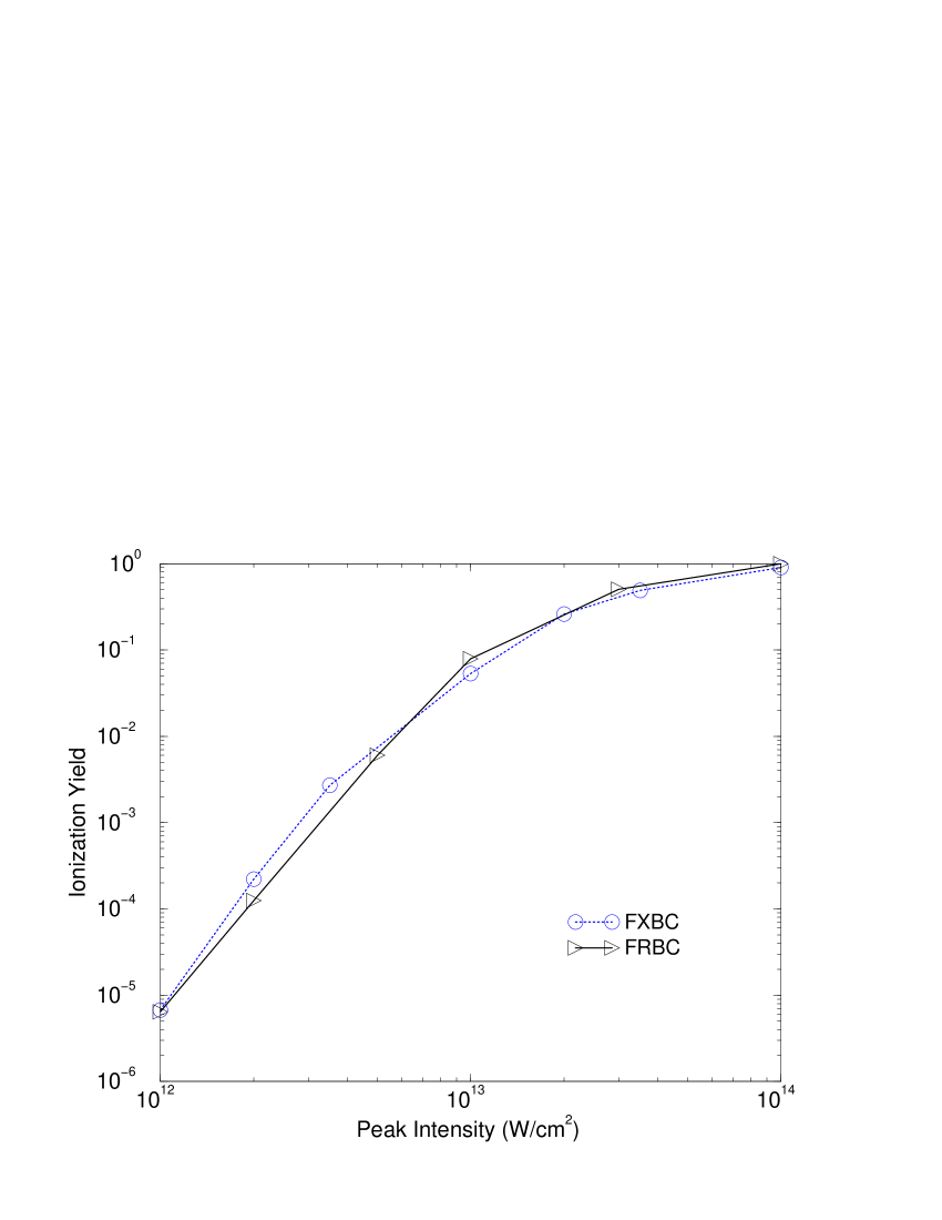
Figure 5:

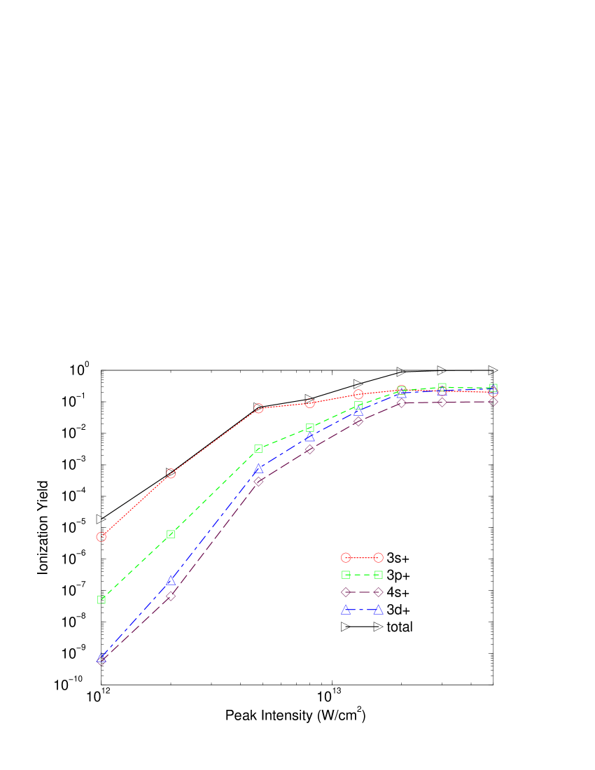
Figure 6:

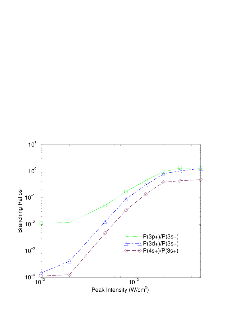
Figure 7:

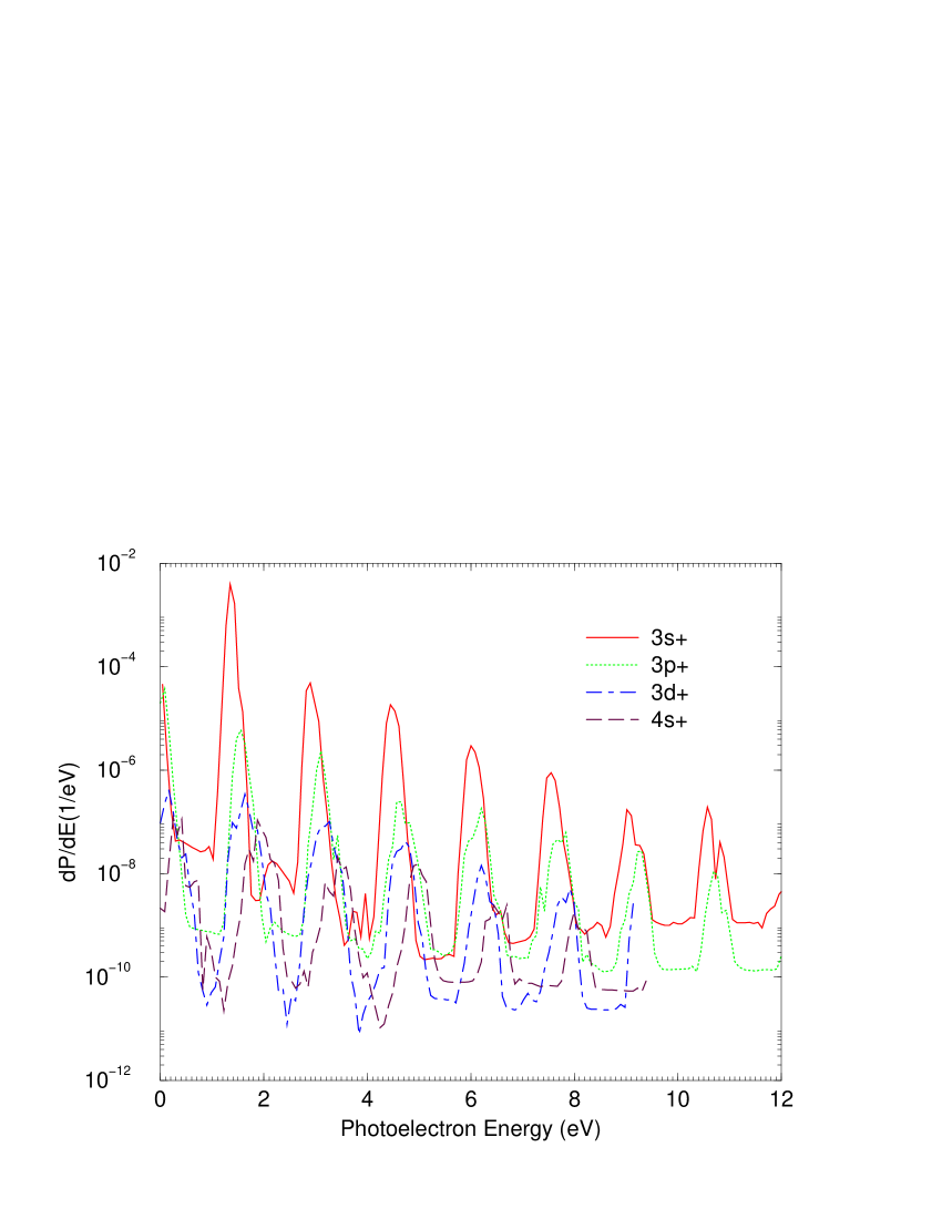
Figure 8: