Using electromagnetic observations to aid gravitational-wave parameter estimation of compact binaries observed with LISA II:

In this follow-up paper, we continue our study of the effect of using knowledge from electromagnetic observations in the gravitational wave (GW) data analysis of Galactic binaries that are predicted to be observed by the new Laser Interferometer Space Antenna in the low-frequency range, $10^{-4}\>\mathrm{Hz}<f<1\>\mathrm{Hz}$. In the first paper, we have shown that the strong correlation between amplitude and inclination can be used for mildly inclined binaries to improve the uncertainty in amplitude, and that this correlation depends on the inclination of the system. In this paper we investigate the overall effect of the other orientation parameters, namely the sky position and the polarisation angle. We find that after the inclination, the ecliptic latitude of the source has the strongest effect in determining the GW parameter uncertainties. We ascertain that the strong correlation we found previously, only depends on the inclination of the source and not on the other orientation parameters. We find that knowing the sky position of the source from electromagnetic data can reduce the GW parameter uncertainty up to a factor of $\sim 2$, depending on the inclination and the ecliptic latitude of the system. Knowing the sky position and inclination can reduce the uncertainty in amplitude by a factor larger than $40$. We also find that unphysical errors in the inclinations, which we found when using the Fisher matrix, can affect the corresponding uncertainties in the amplitudes, which need to be corrected.

1 Introduction

Even though population synthesis studies have predicted $\sim 10^{8}$ galactic white-dwarf binaries (e.g. Nelemans et al. 2001), there are only about $\sim 50$ compact binary sources that have been studied at optical, UV, and X-ray wavelengths (e.g. Roelofs et al. 2010). A space-based gravitational wave (GW) detector, such as the proposed ESA mission eLISA, is expected to observe millions of these predicted compact Galactic binaries with periods shorter than about a few hours (Nelemans 2009; Amaro-Seoane et al. 2012), amongst other astrophysical sources, and resolve several thousands of these binaries (Nissanke et al. 2012). In a recent paper, we investigated the effect of using knowledge from electromagnetic (EM) observations in the gravitational wave data analysis of Galactic binaries by exploring the correlations that might exist between these parameters. We found that for binaries with relatively low inclinations ($\iota\lesssim 45^{\circ}$), an EM constraint on inclination can improve the estimate of the GW amplitude by a significant factor (Shah et al. 2012, Paper I, hereafter). The improvement depends on the signal-to-noise ratio (S/N) of the source and on the EM constraint on inclination itself. We also found that this correlation is a strong function of the inclination of the system, but that it is independent of other angular parameters that describe the binary, in particular, sky position, and polarisation angle. From the initial results we also found that several other correlations that were rather small as a function of inclination (e.g. Figure 4 in Paper I) change drastically when computed as a function of sky position. We address this problem here and also investigate the general dependence of parameter uncertainties on the orientations of the binary. Additionally, we discuss the influence of knowing the sky position from EM data on the parameter uncertainties of the binary sources.

The angular resolution of cLISA for monochromatic binaries has been studied previously (Peterseim et al. 1997; Cutler 1998; Rogan & Bose 2006; Błaut 2011). Peterseim et al. (1997) have shown the uncertainty in ecliptic latitude and ecliptic longitude as a function of both the parameters for a specific case of a cross-polarised source radiating at $f=3\mathrm{mHz}$, which would be observable by cLISA. For a source with $S/N=115$, depending on the values of the ecliptic latitude and longitude, they found the uncertainties in these angles to range from 1 to 8 milliradians. However, they assumed that except for the sky position, all other parameters are known a priori. Their study was also limited by a very simplified detector response and was tailored for a system at an inclination which is favourable in extracting its parameters. Relaxing the assumption of prior knowledge of other parameters, Cutler (1998) has shown that for a binary for a few sets of sky positions, the solid angle uncertainty ($\sigma_{\Omega}$) ranges from 3 to 300 square degrees, depending on the frequency of the source. In subsequent work by Rogan & Bose (2006), sky position uncertainties were estimated for signals modelled for cLISA. They included chirp as an additional parameter, and these signals were not limited to a certain polarisation. Recently, Błaut (2011) has shown sky position uncertainties for various combinations of data channels from cLISA and included detailed detector response for the two distinct cases of low- and high-frequency sources. For a $10^{-3}$ Hz source with an edge-on orientation and an S/N of 10, an observation of one year is predicted to give a solid angle resolution of $\sim 0.1$ steradians which is a result very similar to the study by Rogan & Bose (2006). However, none of these previous authors provided an overall effect of varying multiple angular parameters, which can have a significant effect on parameter uncertainties. In this paper we aim to generalise the uncertainties in all parameters for all possible orientations of the binary and calculate the improvement in these uncertainties that is possible thanks to prior knowledge of the sky position and/or inclination of the system. We show this for eLISA.

A monochromatic binary expected to be observed by eLISA is completely described by seven parameters: dimensionless amplitude ($\mathcal{A}$), frequency ($f$), polarisation angle ($\psi$), initial GW phase ($\phi_{0}$), inclination ($\cos\iota$), ecliptic latitude ($\sin\beta$), and ecliptic longitude ($\lambda$). The inclination of the binary is defined as $\cos\iota=\@vec{n}\cdot\@vec{L}$, where $\@vec{n}$ is the line-of-sight vector from the observer to the source and can be described by the sky position parameters $\beta$ and $\lambda$. $\@vec{L}$ is the orientation of the orbital plane of the binary (or angular momentum vector), which can be specified by $\theta_{L}$ and $\phi_{L}$. One of the main findings of Paper I is that the parameter uncertainties of a monochromatic binary and the three strongest correlations between these parameters (the correlation between amplitude and inclination $c_{\mathcal{A}\>\cos\iota}$, the correlation between phase and polarisation $c_{\phi\psi}$, and the correlation between phase and frequency $c_{f\phi}$) are strong functions of the source’s inclination $\iota$. Furthermore, we found that the parameter uncertainties of such a binary also change as a function of other orientation parameters. These are parameters that describe the relative geometry of the binary in relation to the detector: $\psi$, $\lambda$, and $\beta$. It is natural to then ask the questions, how the possible strong correlations between the parameters due to these four orientation parameters influence these uncertainties, and to which extent knowledge from the EM data can improve the remaining parameter determinations. Of the remaining three parameters, $\mathcal{A}$ (see Eq. 3 in Paper I) is intrinsic to the source and does not depend on its relative orientation to the detector. Since it only scales the S/N of the system, varying the amplitude thus will affect parameter uncertainties as expected, where larger $\mathcal{A}$ will give smaller uncertainties and vice versa. The initial phase $\phi_{0}$, which does not evolve for a monochromatic binary in the eLISA band, has no effect on the signal. On the other hand, the effect of frequency on the parameter accuracies can be significant; the strength of the modulations in the signal (which is caused by the motion of the detector around the Sun and relative to the source) affects low-$f$ sources differently than high-$f$ sources. This has been addressed in detail in previous studies, e.g. Błaut (2011). Hence, here we focus on the effects on the parameter uncertainties of a Galactic binary due to sky position and the orientation parameters.

In this study, we consider low-frequency binaries. We start by briefly summarising the analysis methods and then describe our Monte Carlo (MC) simulations in Section 2. In Section 3, we summarise the important results and our interpretation. In Section 4 we show that uncertainties can be severely overestimated for parameters with clear physical bounds, such as inclination, and thus also for parameters that are tightly correlated with them. We also briefly discuss the S/N limit for which the results are valid in Section 4, and present our conclusions in Section 5.

2 Monte Carlo simulations

Our signal and noise modelling and our data analysis method have been described in Paper I and we briefly summarise them here. The signals from the binaries that are expected to be observed by eLISA are modelled as monochromatic sources characterised by seven parameters, as mentioned above. Most of these sources radiate at low frequencies (milliHertz), including some of the verification binaries like AM CVn, and at these low $f$, the detector response can be derived in the long-wavelength approximation. The noise is composed of instrumental noise described as a Gaussian random process, and a foreground noise mostly arising from the millions of double-detached Galactic white-dwarf binaries. After removing the binaries, which are predicted to be resolved due to their strong signals, the foreground noise is also described by a Gaussian distribution. Given that a signal has a known waveform and the noise is Gaussian, we can use the Fisher matrix to estimate the uncertainties in the parameters that describe the waveform. The inverse of the Fisher information matrix (FIM), known as the variance-covariance matrix (VCM), gives the uncertainties and the correlations between the parameters. Given a number of parameters $n$, one can calculate the $n\times n$ VCM. For details we refer to Paper I.

Uncertainties in parameters are proportional to the inverse of the S/N, but they are also influenced by the correlations between parameters. Generally, a system with higher S/N has smaller parameter uncertainties and vice versa. However, if there is a strong correlation between any two parameters, this (in addition to the S/N) will influence their uncertainties. As mentioned in the previous section, we find that the overall effect of the sky position and the orientation parameters of a binary has not been investigated and this is one of the goals of this study. To do this, we fixed the values of $\mathcal{A}$, $f$, and $\phi_{0}$ to those of AM CVn (see Paper I) and varied its $\psi$, $\iota$, $\beta$, and $\lambda$ within their allowed ranges using a Monte Carlo method. We carried out a number of of MC simulations. Each simulation corresponds to varying a different (sub)set of these four parameters simultaneously. The motivation is to understand how each of the four parameters above influence the GW data analysis individually and in combination with each other. We explain these motivations briefly below, which will become clearer in section 4 where the choice of each MC simulation is explained in more detail.

First of all, we set the distance of the AM CVn system close enough so that the S/Ns are sufficient to believe the Fisher matrix results (see section 4). The first set of simulations we performed for an AM CVn of a fixed $\mathcal{A}$, $f$, and $\phi_{0}$, while its position and orientation parameters $\lambda$, $\beta$, $\psi$, and $\iota$ were all varied simultaneously 4000 times. Thus, from the sample of these 4000 systems with various orientation parameters we first ascertained that the dominant effect on the parameter uncertainties is indeed the inclination of the system (result from Paper I). Next, we can quantify how the other three angles affect the parameter uncertainties globally. We performed another set of calculations where we fixed inclination (to a few choices explained later), frequency, and the phase (like above), and we varied the amplitude (by changing the distance, $d$), the sky position, and the polarisation angle. For each choice of the inclination, MC simulations were performed for 500 systems to quantify the effect of varying the S/N (by changing the distance) and the ecliptic latitude, longitude, and the polarisation angle on the parameter uncertainties. Finally, to quantify the possible improvement in the parameter uncertainties gained by prior (EM) knowledge of the sky location, we carried out 500 MC simulations for an AM CVn at a fixed inclination and varied the rest of the orientation parameters and the distance. However, instead of a full $7\times 7$ VCM, we calculated a $5\times 5$ VCM, where for each system the randomly chosen sky locations were fixed to that value. Similarly, we repeated this exercise to quantify the improvement in the parameter accuracies gained by EM knowledge of inclination in addition to sky position, and thus we calculated a $4\times 4$ VCM for each system. For clarity, we briefly summarise these four sets of MC simulations below:

1. MC1: Fix $\mathcal{A}$ (i.e. $d$, $m_{1}$, and $m_{2}$ where, $m_{i}$ is the mass), $f$, and $\phi_{0}$. Randomly pick the orientation of the binary, $\@vec{L}(\phi_{L},\theta_{L})$, $\lambda$, and $\beta$ over their physical ranges. The parameters $\psi$, and $\iota$ are then given by the following equations (Cornish & Rubbo 2003):

   $$\cos\iota=\cos(\theta_{L})\;\sin(\beta)+\sin(\theta_{L})\;\cos(\beta)+\cos(\phi_{L}-\lambda)\>\;\mathrm{and}$$ (1)

   $$\tan\psi=\frac{\sin\beta\;\cos(\lambda-\phi_{L})-\cos(\theta_{L})\;\sin(\theta_{L})}{\sin(\theta_{L})\;\sin(\lambda-\phi_{L})}.$$ (2)

2. MC2: For each $\iota=30^{\circ},60^{\circ},90^{\circ}$, randomly pick $\lambda$, $\beta$, $\psi$, and $d$.

3. MC3: Like MC2, but fix $\lambda$, and $\beta$ assuming an a priori known sky position [$5\times 5$ FIM].

4. MC4: Like MC2, but fix $\lambda$, $\beta$, and $\iota$ assuming an a priori known sky position and inclination [$4\times 4$ FIM].

Each of the four parameters are randomly picked from their uniform distribution in the following range: $\lambda\in[0,2\pi]$, $\sin\beta\in[-1,1]$, $\phi_{L}\in[0,2\pi]$, $\theta_{L}\in[0,\pi]$, and $d\in[0.01,0.3]$ kpc. The corresponding ranges in $\iota$ and $\psi$ are $[0,\pi]$. We also define the following inclinations for presenting the results below (unless specified): face-on:= $0^{\circ}\leq\iota\leq 45^{\circ}$ or $135^{\circ}\leq\iota\leq 180^{\circ}$, mildly face-on:= $45^{\circ}\leq\iota\leq 60^{\circ}$ or $120^{\circ}\leq\iota\leq 135^{\circ}$, mildly edge-on:= $60^{\circ}\leq\iota\leq 80^{\circ}$ or $100^{\circ}\leq\iota\leq 120^{\circ}$, and edge-on:= $80^{\circ}\leq\iota\leq 100^{\circ}$.

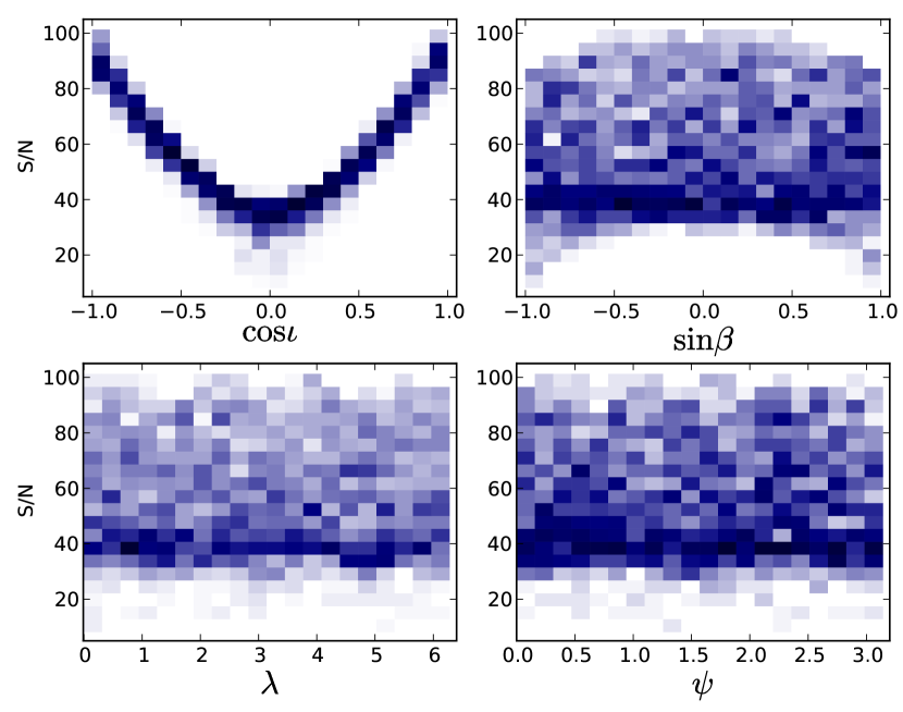
Figure 1: Two-dimensional distributions of signal-to-noise ratio as a function of $\cos\iota$, $\sin\beta$, $\lambda$, and $\psi$. Face-on, mildly face-on, mildly edge-on, and edge-on systems (whose exact bounds are specified in Section 2) can be read off from the top-left panel. In the other panels, the trend from face-on to edge-on systems follows from the top of the distribution to the bottom.

3 Results

3.1 Global dependence of the uncertainties: dominance of inclination (MC1)

We have seen in Paper I that the parameter uncertainties are a strong function of the inclination of the system, which is due to the strong dependence of the signal strength, i.e. S/N, on the inclination and to the strong correlations. In this section, we first discuss the global behaviour of the parameter uncertainties as a result of varying the sky position, inclination, and the polarisation angle at the same time. We verify the result from Paper I that inclination has a dominant effect on the parameter uncertainties. We show that after the inclination, the ecliptic latitude, $\beta$, of the system has the strongest influence on the parameter uncertainties.

Using the results from MC1, we show in Figure 1 the S/N of binary systems as a function of the four angular parameters over which they are randomly picked. As expected, there is a strong dependence of S/N of a system on inclination, as shown in the top-left panel. Due to this dependence on the inclination, in the other panels we find that the face-on systems form a band at the top of these plots, followed by bands of mildly face-on, mildly edge-on, and edge-on systems, in that order. In the top-right panel, there is a mild but noticeable increase in S/N, for the binaries at the ecliptic plane, $\sin\beta=0$, whereas the ecliptic longitude and the polarisation angle have no significant effect on the binaries’ S/N, as shown in the bottom panels. Figure 2 is a plot of parameter uncertainties as a function of $\sin\beta$ taken from MC1. In the top panels, uncertainties in $\mathcal{A}$, $\iota$, $\phi$, and $\psi$ are smallest for edge-on systems (forming a band at the bottom) and progressively increase for the face-on systems (the top of distribution). This is discussed in Paper I and results from the correlations between these parameters. The lower inclination systems $\iota\lesssim 45^{\circ}$ or $\iota\gtrsim 135^{\circ}$ have very similar signal shapes in those ranges, whereas systems with close to edge-on orientations are distinguishable by both the shape and structure for small differences in inclinations. For face-on systems a small change in inclination is indistinguishable from a small change in its intrinsic amplitude, whereas for an edge-on system, a small change in inclination produces a noticeably different signal. Thus even for their lower S/Ns, the inclinations of the edge-on systems are better determined than those of the face-on systems. A similar argument based on the strong correlation between $\phi$ and $\psi$ for face-on systems can explain the huge uncertainties of these parameters despite their strong signals (see Paper I). Since there are no such correlations between $f$, $\lambda$, and $\beta$ (or the solid angle $\Omega$), their uncertainties should be a consequence of the S/N, i.e. from the top panels of Figure 1: a higher S/N implies lower values for the uncertainties and vice versa, which indeed holds for $\sigma_{f}$ and $\sigma_{\lambda}$. From Figures 1 and 2 it is evident that inclination has the strongest effect on the S/N and so to the leading order this parameter affects the parameter uncertainties, which confirms our results in Paper I.

After inclination, the strongest effect on the S/N of the systems is produced by the ecliptic latitude. Thus, we expect the uncertainties in the parameters also to be affected by $\beta$ (see top-right panel in Figure 1); sources at the ecliptic poles should have larger uncertainties than those at the ecliptic plane. In Figure  2 we can see that for a fixed distance to the source $d$, most uncertainties ($\sigma_{\mathcal{A}}$, $\sigma_{\iota}$, $\sigma_{\phi}$, $\sigma_{\psi}$, $\sigma_{f}$, and $\sigma_{\lambda}$) are indeed smaller towards the plane than close to the poles. This is probably largely due to the S/N as a function of $\sin\beta$. The unusual behaviour of $\sigma_{\beta}$, which increases at the plane compared to its value at the poles ($\sin\beta=\pm 1$), has been pointed out in Cornish & Larson (2003) and is caused by the Doppler modulation $\Phi_{\mathrm{D}}$ (Eq. 9 in Paper I). This behaviour is surprising since $\Phi_{\mathrm{D}}$ has the largest magnitude on the plane (since it is proportional to $\cos\beta$), and so we naively expect the sky resolution to be better on the ecliptic plane. However, the resolution in $\beta$ is determined by the rate of change of the Doppler modulation with respect to $\beta$ (i.e. proportional to $\sin\beta$), which is the highest at the pole and lowest at the plane. This is also evident in the solid angle uncertainty $\sigma_{\Omega}$ in the bottom-right panel in Figure 2, where $\sigma_{\Omega}=2\pi(\sigma_{\sin\beta}\sigma_{\lambda}-\mathcal{C}_{\sin\beta\lambda})$, $\mathcal{C}_{\sin\beta\lambda}$ being the unnormalised correlation between $\sin\beta$ and $\lambda$ (Cutler 1998). We also observe that $\sigma_{\lambda}$ has a distinct U shape, becoming very severe at the poles. This is merely because $\lambda$ becomes progressively less well-defined as a source lies closer to the pole. Note that at the pole $\lambda$ is not defined, which means that it can take any value.

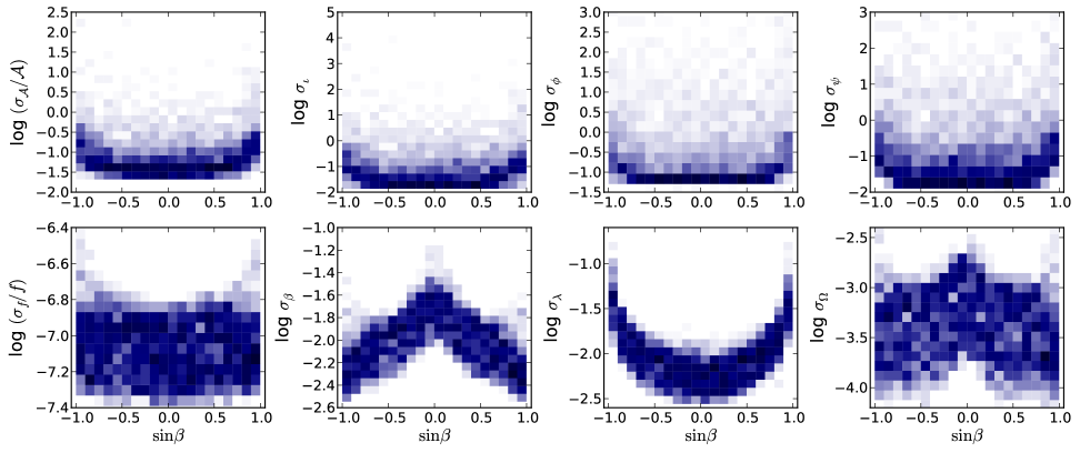
Figure 2: Two-dimensional distributions of the uncertainties in the seven GW parameters of the galactic binary systems as a function of $\sin\beta$ from MC1 as described in the text. Units of the angles are in radians.

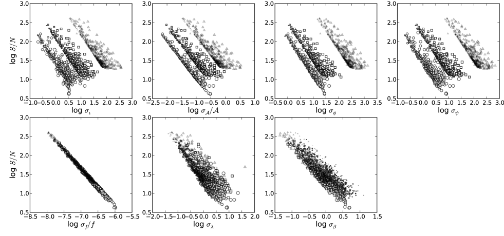
Figure 3: Uncertainties in all seven parameters of the systems as a function of S/N from MC2. Open circles, squares, and filled triangles represent binary systems at fixed inclinations of $90^{\circ},60^{\circ},$ and $30^{\circ}$ respectively. The size of the symbol represents the magnitude of $|\beta|$ for each simulated binary. In the bottom panels the different groups of symbols overlap.

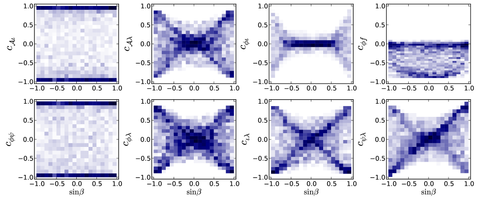
Figure 4: Two-dimensional distributions of the normalised correlations as a function of $\sin\beta$ from MC2. We show here only the strong (normalised) correlations, meaning $|c_{ij}|>0.5$.

3.2 Dependence of the uncertainties on $\beta$: S/N or correlations (MC2)?

The general behaviour of the parameter uncertainties (except $\sigma_{\beta},$ hence $\sigma_{\Omega}$) in Figure 2 shows a minimum at the ecliptic plane that could be attributed to the S/N, since it is the highest for sources in the plane. To investigate this change in the uncertainties as a function of $\sin\beta$, we consider the results from MC2 and the correlations between parameters from MC1. In MC2 we varied S/N (by varying the distance to the binary, $d$), $\lambda$, $\beta$, and $\psi$ for a few fixed inclinations. We fixed the $\iota$ for each of the MC2 simulations because we established its dominant effect through the S/N in the previous section, therefore the goal now is to determine which contributes most to the behaviour observed in Figure 2: the S/N (top-right panel of Figure 1), or the correlations as a function of $\sin\beta$. If the larger uncertainties at the pole compared to the plane are solely due to the corresponding S/Ns, then we should see from the MC2 simulations that uncertainties anti-correlate tightly with the S/N of the sources. In Figure 3 we show three distinct curves in S/N vs. parameter uncertainty that roughly show monotonic functions where all the uncertainties decrease with increasing S/N. However, all uncertainties except $\sigma_{f}$ have a significant horizontal scatter. In the figure, the size of the symbol represents the magnitude of the ecliptic latitude. Higher values of $|\beta|$, which represent regions around both ecliptic poles, concentrate towards the right-hand side of the plots (with the exception of $\sigma_{\beta}$), and the opposite is true for the lower values of $|\beta|$, which roughly represent the ecliptic plane. In the top panels, from left to right, the curves correspond to $\iota=90^{\circ},60^{\circ}$, and $30^{\circ}$ respectively, and these overlap in the bottom panels. As explained above, $\sigma_{\mathcal{A}}$, $\sigma_{\iota}$, $\sigma_{\psi}$, and $\sigma_{\phi}$ are larger for face-on systems ($\iota=0,30^{\circ}$) than for edge-on systems ($\iota=90^{\circ}$), owing to the correlations between these parameters even though face-on systems have higher S/Ns. Since these correlations are very weak for $\lambda$, $\beta$, and $\psi$ for all inclinations (see Paper I), their uncertainties overlap in the bottom panels of Figure 3. This spread across the horizontal axis must be due to changes in their correlations as a function of the ecliptic latitude. This is indeed shown in Figure 4, which is taken from MC1. In the figure we show a 2d histogram to display the global dependency of the correlations on the ecliptic latitude. We notice that the correlations involving $\lambda$, $\iota$, $\psi$, $\phi$, and $\mathcal{A}$ ($c_{\mathcal{A}\lambda}$, $c_{\phi\iota}$, $c_{\phi\lambda}$, $c_{\iota\lambda}$, and $c_{\psi\lambda}$) are generally weaker at the ecliptic plane. However, at the poles these correlations can take any value from 0 to $\pm 1$ and concentrate at $\pm 1$. This is the case for all inclinations. Accordingly, close to the ecliptic poles, there are sets of $\lambda$ and $\psi$ for which the correlations can become very strong, which explains the horizontal spread of uncertainties in Figure 2. Note that in Figure 4, we have shown (only) the normalised correlations $c_{ij}$, whose absolute values can exceed 0.5. A detailed explanation of these correlations can be found in the Appendix.

3.3 Gain from a priori knowledge of sky position and inclination (MC and MC4)

From Figures 2 and 3 we observe that uncertainties in sky location are rather large (which has also been pointed out in previous studies). For the S/Ns in this study ($\sim 8-100$), the uncertainties in $\sigma_{\Omega}$ range from $\sim 0.2$ to $6$ square degree, as shown in Figure 1. If EM data can provide a more accurate sky position and possibly an inclination for AM CVn system, we can use these independent (EM) measurements to improve accuracies in other parameters. To see by which factors the uncertainties improve, we fixed the sky position of each source and calculated the corresponding $5\times 5$ VCM. The ratios of uncertainties from using a $7\times 7$ VCM to using a $5\times 5$ VCM, i.e. the improvement when knowing the sky position (ecliptic latitude and longitude) exactly, are shown in Figure 5, calculated from MC2 and MC3. In the figure, the size of the symbol represents the S/N of that system. The figure shows that the improvement factor depends on the inclination of the source: for edge-on systems (in open circles with $\iota=90^{\circ}$) $\sigma_{\psi}$ can improve by a factor of $\sim 3$, but for systems closer to a face-on configuration in squares and filled triangles the improvement can only be up to a factor of $\sim 2.2$. One useful result from this figure is that $\sigma_{\mathcal{A}}$ and $\sigma_{\iota}$ can improve by a factor of $\sim 2$ for the systems close to the ecliptic poles. This gives a motivation for independent EM observations of the sky location. However, for edge-on systems there is no improvement in $\sigma_{\mathcal{A}}$ even though $\sigma_{\iota}$ improves. This is simply due to the lack of correlation between these two parameters for $\iota=90^{\circ}$.

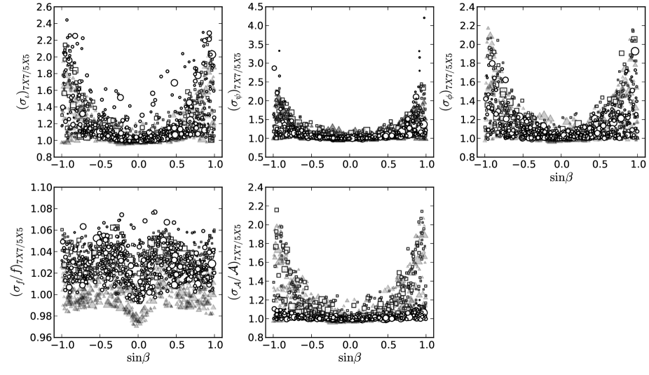
Figure 5: Uncertainty ratios of the parameters between analyses using a $7\times 7$ VCM and a $5\times 5$ VCM, where the sky position is fixed in the latter, as a function of $\sin\beta$ (from the MC2 and MC3 simulations). Filled triangles, squares and open circles represent systems at fixed inclinations of $30^{\circ},60^{\circ}$ and $90^{\circ}$ respectively. The size of the symbol for each binary represents the S/N of the system.

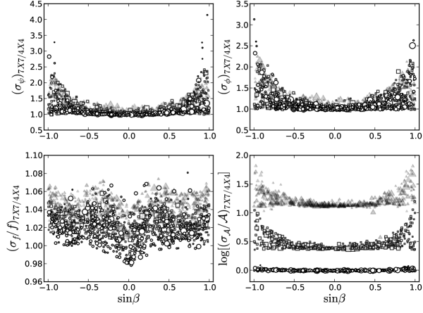
Figure 6: Same as in Figure 5 but now we assume that in addition to sky position we also know the inclination of the binary. The uncertainty ratios of the parameters are between $7\times 7$ VCM (MC2) and $4\times 4$ VCM (MC4). The improvement factors in amplitude include corrections due to overestimated uncertainties in the amplitudes of face-on systems (see Section 4.1) Note that the last panel is plotted in log scale in order to highlight the relatively large improvements for the systems with smaller inclinations.

In Paper I we found that for the HM Cnc system, the improvement of $\sigma_{\mathcal{A}}$ by using the EM constraint in $\iota$ was smaller than for AM CVn, although the two have similar inclinations (thus the same (normalised) correlation between $\mathcal{A}$ and $\iota$). This was due to the relatively high S/N of HM Cnc compared to the latter and thus the individual improvement factors shown in Figures 5 and  6 will also depend on the individual S/N of the systems (see Paper I).

If in addition to sky position the inclination can be constrained, as discussed previously in Paper I, the improvement factor in amplitude can be much larger because of the decoupling of the correlation between amplitude and inclination. We show the ratio of parameter uncertainties from calculating the $7\times 7$ VCM to the uncertainties from a $4\times 4$ VCM (where $\lambda,\>\beta$ and $\iota$ are fixed) in Figure 6. The improvements in $\sigma_{\psi}$ and $\sigma_{\phi}$ are roughly similar to the case in Figure 5. A remarkable difference is seen in the improvement of $\sigma_{\mathcal{A}}$ for binaries with $\iota=30^{\circ}$ represented in filled triangles plotted in the bottom-right panel of Figure 6. This is expected because by fixing $\iota$, the strong correlation between amplitude and inclination is decoupled. Hence for the higher S/Ns of close to face-on systems, the uncertainties in $\mathcal{A}$ is significantly reduce. Note that here we assumed that the inclination is known exactly.

4 Discussion

4.1 Limiting inclinations to their physical range

Some of the uncertainties in $\iota$ in Figure 2 from MC1 are noteworthy in that they exceed their physical bounds, for example $\sigma_{\iota}=7$ radians. The cause for this is that the linearised signal approximation that is internally employed in the Fisher matrix studies is not sensitive to the bounded parameters that describe the model signal, as has been pointed out in Vallisneri (2008). Thus, when an uncertainty in a (cyclicly) bounded parameter like the inclination exceeds its physically allowed range, it means the quantity cannot be determined from GW data analysis alone. For the parameter $\iota$, we can further ask what the unphysical uncertainty in $\iota$ implies for the uncertainty in $\mathcal{A}$ for the mildly inclined systems that has a strong correlation between the two parameters. Since the Fisher matrix estimates $\sigma_{\iota}$ to unphysical values while in reality it is constrained within $[0^{\circ},90^{\circ}]$, does this mean that the uncertainty in the amplitude (due to the correlation with $\iota$) is also overestimated? Or should we not trust the uncertainty in all those parameters where the $\sigma_{\iota}$ becomes unphysical?

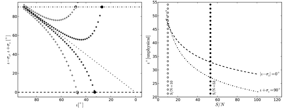
Figure 7: Left: 1-$\sigma$ uncertainty in the inclinations vs. source inclinations for two values of S/N: plusses (outer curves) correspond to S/N=10, stars (inner curves) correspond to S/N=53. The curves above the dotted line correspond to $\iota+\sigma_{\iota}$, and those below to $\iota-\sigma_{\iota}$. The thick horizontal dashed and dashed-dotted lines are the physical limits of $\iota$: below the line of $\iota\pm\sigma_{\iota}=0^{\circ}$ and above the line of $\iota\pm\sigma_{\iota}=90^{\circ}$, $\sigma_{\iota}$ can be truncated, since that value of $\iota$ is bounded between $[0^{\circ},90^{\circ}]$. Right: ‘Unphysical $\iota$’ versus S/N for the systems from MC1. The thick dashed-dotted line calculated from the condition $\iota-\sigma_{\iota}=0^{\circ}$, and the thick dashed line from the condition $\iota+\sigma_{\iota}=90^{\circ}$ demonstrated in the left panel. At an S/N of 10, the in open circles show a lower limit and the filled circles show an upper limit at the intersections with the two curves from the conditions above.

Consider the $\mathcal{A}-\iota$ error ellipse for a given signal $h$, with true signal values $\iota_{0}$ and $\mathcal{A}_{0}$, where the two parameters are strongly correlated and where $\sigma_{\iota}>>\pi$. The corresponding accuracy $\sigma_{\mathcal{A}}$ is then also highly inflated. Now consider a second signal $h(\mathcal{A}_{1},\iota_{1})$, inside the error ellipse, but far from the true values, and such that $\iota_{1}$ = $\iota_{0}+2n\pi$ with $n>1$. From its cyclic behaviour, $h(\mathcal{A}_{1},\iota_{1})=h(\mathcal{A}_{1},\iota_{0})$ should hold. However, this last point would typically lie far outside the error ellipse in the $\mathcal{A}-\iota$ plane, which would indicate that this is actually a signal that is very dissimilar to the true signal. Hence, the fact that the inclination is physically limited to the range $[0,\pi]$ and that this is not taken into account in the FIM method means that we should not only limit the uncertainty in inclination to its physically allowed range, but that we should limit the uncertainty in amplitude accordingly. Specifically, the corrected amplitude uncertainty, $\sigma_{\mathcal{A}}^{\prime}$, is given by,

$$\sigma_{\mathcal{A}}^{\prime}=\sigma_{\mathcal{A}}[\mathrm{VCM}]\times\frac{\sigma_{\iota}^{\prime}}{\sigma_{\iota}[\mathrm{VCM}]},$$ (3)

where $\sigma_{\iota}^{\prime}$ is the corrected inclination uncertainty.

The value of inclination where its uncertainty becomes unphysical can occur at two places, i.e. where $\iota+\sigma_{\iota}>\pi/2$ , and/or $\iota-\sigma_{\iota}<0$, as shown in the left panel of Figure 7. In the panel, the 1-$\sigma$ uncertainty ranges of the inclination are plotted against the sources’ inclination for two cases of constant S/N of 10 and 53. The thick horizontal dashed and dashed-dotted lines indicate the conditions where $\sigma_{\iota}$ becomes unphysical. At a fixed S/N of 10 (in plusses), these values are at $\iota\sim 48^{\circ}$ and $\iota\sim 47^{\circ}$, respectively, as indicated by the open circles, whereas for a higher S/N of 53 (in stars) the above conditions for $\sigma_{\iota}$ occur at $\iota\sim 27^{\circ}$ and $\iota\sim 32^{\circ}$ indicated by filled circles. We calculated the inclinations at which these intersections occur for a range of S/Ns, $10-110$ and show the results in the right panel of Figure 7. These curves can be used to apply corrections to the limits of $\sigma_{\iota}$ in Figure 2 from MC1, which in turn can be used to limit $\sigma_{\mathcal{A}}$ from Eq. 3. In Figure 8 we compare the uncertainties in $\mathcal{A}$ corrected in this way with those from Figure 2. The corrected values for $\sigma_{\mathcal{A}}$ differ for the high S/N systems, as can been seen by comparing the two right-hand panels in Figure 8. In particular, the tail at the large $\sigma_{\mathcal{A}}/\mathcal{A}$ present in the top panel is absent from the bottom panel.

There is a caveat to applying these corrections. In the left panel of Figure 7 we can understand the cut-off at $0^{\circ}$ at the bottom of the figure. However, at the top, the cut-off of $90^{\circ}$ is not so clear. A system with a lower inclination (e.g. $20^{\circ}$) cannot have an error larger than $\sim 50^{\circ}$ because a system with an inclination in the range $\sim 80^{\circ}-90^{\circ}$ is distinguishable from a system with an inclination of $\sim 0-60^{\circ}$, as has been pointed out in Paper I. Thus the cut-off of $\iota+\sigma_{\iota}=\pi/2$ for lower inclinations is a conservative estimate. The estimated posterior probability distribution functions (PDFs) obtained using the FIM do not predict the real PDFs for lower inclinations and lower S/Ns. Thus a full Bayesian analysis that takes into account the limits of the cyclic parameters as priors is needed to fully determine the PDF. This is beyond the scope of this paper, and we used these (probably) over-estimated uncertainties to give the corresponding bounds in the amplitude.

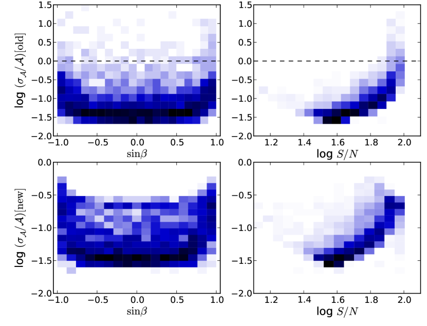
Figure 8: Corrections applied to the uncertainties in amplitude and inclination from Figure 2. The row titled ‘new’ was produced using the curves from the right panel of the Figure 7 on MC1 simulations.

In the same manner that $\sigma_{\mathcal{A}}$ was corrected in Figure 8, we corrected for the MC2 calculations. The predicted improvement factors of the amplitude in the bottom-right panel of Figure 6 already include the corrections mentioned above.

4.2 Use of FIM at S/N $\sim 15$

Another problem regarding the trustworthiness of the Fisher matrix is the limit of the S/N at which one can trust the values from VCM matrix. This has been addressed in Nicholson & Vecchio (1998), where the authors have performed Fisher matrix studies in predicting the uncertainties of the parameters of the coalescing binaries. They have compared these predictions with calculations from Bayesian uncertainties, and their main finding is that above an S/N of 15, the uncertainties from the Bayesian calculations converge to Fisher matrix predictions. At an S/N of 10, the analytic predictions of Fisher matrix deviate by about $6\%$ and at a lower S/N of 7, they increase to about $25\%$. For MC1, the lowest S/N we considered is above $\sim 15$, as indicated in Figure 1, and consequently the results following MC1 are reasonable. However, real observations for eLISA will of course also contain lower S/Ns.

5 Conclusion

We presented a follow-up study of correlations between parameters that characterise Galactic binaries that will be observed by eLISA in the frequency range $10^{-4}\>\mathrm{Hz}<f<1\>\mathrm{Hz}$. In Paper I we investigated the correlations between parameters by considering three of the verification binaries (which are already known optically and are thus guaranteed sources for eLISA), and we explained these correlations and parameter uncertainties as a function of the inclination of the system. In this paper, we addressed the effect of all position and orientation parameters on the uncertainties and the possible strong correlations between them. We found that the overall effect is dominated by sky position and explained that dependence. Our main conclusions are:

1. After inclination, the ecliptic latitude of the source has the strongest influence on its parameter uncertainties, mainly due to its dependence on the signal-to-noise ratio and the correlations that can become very strong at the poles. For a given source distance, the parameter uncertainties (except for $\sigma_{\beta}$) are larger for a source at the ecliptic pole than for a source at the ecliptic plane. This is because a signal received from a source at the plane is stronger than that from a source at the pole.

2. In general, the uncertainty in sky location $\sigma_{\Omega}$ is large, i.e. in the order of square degrees. By constraining $\lambda$ and $\beta$ from optical data, the uncertainties in $\psi$, $\phi$, $\iota$, and $\mathcal{A}$ in the GW analysis can be improved by a factor of $\sim 2$. This factor is dependent on the inclination and the ecliptic latitude of the system.

3. By constraining $\iota$ in addition to the sky location, the improvement in $\sigma_{\mathcal{A}}$ is remarkably large (factors of 10 depending on the S/N of the source). Systems with $\iota=30^{\circ}$ can have improvement factors as high as 60.

4. The remaining angular parameters $\lambda$ and $\psi$ do not influence the correlations or uncertainties significantly.

5. The uncertainties in amplitude for low-inclination systems for which the corresponding uncertainties in the inclinations are unphysical (i.e. beyond their physical bounds) are also exaggerated. Fisher matrix predictions for these uncertainties have to be corrected for such systems.

Appendix A Correlations as a function of $\beta$

We found that several correlations between source parameters become amplified at certain ecliptic latitudes and thus are a strong function of $\beta$, as shown in Figure 4. Several of these correlations do not have preference on the inclination of the system, and therefore we show a 2d histogram to show the dependency on the ecliptic latitude. In the figure we show (only) the correlations that become strong, i.e. where the normalised correlation $|c_{ij}|>0.5$. Some of these correlations have been explained in Paper I and are only dependent on the inclination of the system; we show them here to confirm that claim. The remaining correlations and their dependency on the latitude can be understood by considering the orientation of the binary relative to the detector. We comment on or explain each of them below,

1. $c_{\mathcal{A}\iota}$: Explained in Section 3.1.

2. $c_{\phi\psi}$ and $c_{\phi f}$: Similarly to $c_{\mathcal{A}\iota}$, these are strongly influenced by the source’s inclination. The correlation $c_{\phi\psi}$ in the bottom-left panel has a distribution that looks very similar to the case of $c_{\mathcal{A}\iota}$ and here too, phase and polarisation are strongly correlated for face-on and mildy face-on systems, since these two angles describe similar properties. For edge-on systems, the two angles are defined on two planes that are perpendicular to each other, making them distinct. The correlation $c_{\phi f}$ in the top-right panel is strong for edge-on systems because a small shift in phase is very similar to a small change in frequency. However, for face-on systems, the phase and frequency become degenerate owing to the uncertainty in $\phi$, which is inflated due to the strong correlation with $\psi$. There is a slight dependency of this correlation on $\sin\beta$ for the edge-on orientations since the correlation has a larger spread at the ecliptic poles. This is due to the spread of the $c_{\phi\psi}$ for $\iota>80^{\circ}$ systems where the spread in the phase at the poles also inflates the frequency. However, $\iota<60^{\circ}$, $c_{\phi\psi}$ for has no such spread, and thus the distribution of $c_{\phi\psi}$ vs. $\sin\beta$ for these systems lies in a narrow band throughout.

3. $c_{\psi\lambda}$: This can be understood by considering a binary with $\iota=90^{\circ}$ close to one of the poles; rotating the binary about its line-of-sight is equivalent to changing its $\psi$ and $\lambda$ because they are defined on the same plane (perpendicular to the line-of-sight). This also holds for a face-on binary, and thus if a source is close to the poles, $\psi$ and $\lambda$ can be highly correlated. The spread of this correlation is most likely due to the fact that $\lambda$ is not well defined at the poles and thus the inflated uncertainty in the longitude implies a spread of correlations at the poles.

4. $c_{\phi\lambda}$: This correlation is explained by the combination of $c_{\psi\lambda}$ and $c_{\phi\psi}$, which are explained above. Since $\psi$ and $\lambda$ can be highly correlated at the poles and $\phi$ and $\psi$ are strongly correlated for face-on systems, we found that $\phi$ and $\lambda$ should also be highly correlated at the poles, at least for the systems with (mildly) face-on orientations. For the edge-on systems, this strong correlation can also exist because even though $c_{\phi\psi}$ is not as strong in this case, the values of this correlation (as pointed out above) spread at the poles for $\iota=90^{\circ}$. This spread is responsible for the spread of $c_{\psi\lambda}$ around the poles for edge-on systems.

5. $c_{\iota\lambda}$ and $c_{\mathcal{A}\lambda}$: A strong correlation between inclination and the longitude is intuitively not as clear. However, this correlation combined with $c_{\mathcal{A}\iota}$ for face-on systems would explain the correlation between amplitude and longitude, $c_{\mathcal{A}\lambda}$.

6. $c_{\phi\iota}$: Like above, the correlation between phase and inclination follows from the combination of $c_{\phi\lambda}$ and $c_{\iota\lambda}$, both of which are stronger close to the poles.