Charmless $B_{u,d,s}\to VT$ decays in perturbative QCD approach

Abstract

Motivated by the experimental data, we study charmless $B_{u,d,s}\to VT$ ($V$ and $T$ denote light vector and tensor mesons respectively) decays in the perturbative QCD approach. The predictions of branching ratios, polarization fractions and direct CP violations are given in detail. Specifically, within this approach we have calculated the polarization fractions and the branching ratios of $B\to\phi(K_{2}^{*-},\bar{K}_{2}^{*0})$ which agree well with the observed experimental data, however the branching ratios of $B\to\omega(K_{2}^{*-},\bar{K}_{2}^{*0})$ are hard to be explained, where the polarization fractions are well accommodated. The tree dominated channels with a vector meson emitted have longitudinal polarization fraction of $90\%$, while the penguin dominating ones have subtle polarization fractions. Fortunately, most branching ratios of $B_{u,d}$ decays are of the order $10^{-6}$, which would be straight forward for experimental observations. For the $B_{s}$ decays the branching ratios can reach the order of $10^{-6}$ in tree dominated decays, while in penguin dominated decays those are of order of $10^{-7}$ which require more experimental data to be observed.

1 Introduction

Flavor physics has been being thoroughly investigated for many years with the advent of $B$-factories. As more and more experimental data is accumulated, flavor physics plays an important role in the precision test of the standard model (SM) and beyond the SM as well as studying the properties of many light hadrons. A few $B\to VT$ decay channels have been already reported by the BaBar collaboration Aubert:2009sx ; Aubert:2008bc ; Aubert:2008zza , which makes the $B$ to tensor meson decays gain more and more attention.

Even before the experimental reports there had been already a couple of works LopezCastro:1997im ; Munoz:1998sn , which studied the $B\to VT$ decays involving a charmed tensor meson under the quark model. Here we would like to consider the charmless $B\to VT$ decays instead. As early works, these charmless decays had been also studied in the framework of generalized factorization Kim:2001py and in Isgur-Scora-Grinstein-Wise updated model Kim:BtoVT . Later these decays were again studied in the covariant light-front approach in Ref. JHMunoz:2009aba . Polarizations of $B\to VT$ decays as well are studied in Ref. Datta:2007yk . However, most of the branching ratios in the early works are not predicted precisely, which are usually one or two order smaller than the experimental data. This may indicate that some contributions, such as the nonfactorizable and annihilation contributions, are very important in these decays, which are not included in those early works. It has become very urgent to investigate these contributions by employing proper theoretical models. In Ref. Cheng:2010yd the authors accommodated the experimental data with the QCD factorization (QCDF) approach Beneke:QCDF , which deals with these additional contributions in a very subtle and technical way. Here we want to adopt yet another theoretical approach, the perturbative QCD (pQCD) approach HNLi:pQCD , which calculate the nonfactorizable and annihilation contributions in a theoretically systematical way. These investigations will offer us more detailed knowledge about the dynamics of $B\to VT$ decays, which is one reason why those decays are worthy to be studied again.

Another reason why $B\to VT$ decays are meaningful is the interesting polarization phenomena. In $B\to VV$ decays, the transversely polarized contributions of some penguin dominating channels, such as $B\to(\phi,\rho)K^{*}$, are nearly the same as the longitudinal ones Amsler:2008zzb . This is quite different from the prediction of the naive factorization, in which the longitudinal polarization always dominates. However, in $B\to VT$ decays, such as $B\to\phi K_{2}^{*}$, the experimental data indicate that the longitudinal polarization is much larger, while for $B\to\omega K_{2}^{*}$ the longitudinal polarization takes only about a half contribution. Earlier models such as naive factorization cannot give us any satisfied explanation. Therefore, employing theoretically more complete models, such as the QCDF, the pQCD and the soft collinear effective theory, to understand the phenomena becomes very important.

In a recent paper Cheng:2010hn , the authors studied the light cone distribution amplitudes of the tensor mesons, which make the calculation of $B\to VT$ decays possible for the QCDF and the pQCD approach. In their following paper Cheng:2010yd , by extracting inputs from the experimental data they accommodated $B\to VT$ decays in the frame of the QCDF. However, some subtle dynamical phenomena is not yet fully understood, which inspires us to explore these decays under another approach. The pQCD approach based on the $k_{T}$ factorization has already been used to explore many two body exclusive decays of $B$ meson. The form factors of $B$ to a tensor meson transition has already been calculated under this approach Wang:2010ni . There are already a few investigations on the $B$ to a pseudoscalar and a tensorZou:2012td as well as a charmed meson and a tensor meson decays Zou:2012zk ; Zou:2012sx ; Zou:2012sy . Though there still exist few controversies DescotesGenon:2001hm ; Feng:2008zs on its feasibility, the predictions based on the pQCD can accommodate many experimental data well, for example, see Ref. Li:2004ti . In this work, we will put the controversies aside and adopt this approach to our analysis.

The paper is organized as follows. In Sec. 2, all the details of the theoretical frameworks are listed, including the notation conventions, the Hamiltonian, the kinematics definitions, the wave functions which are used as the inputs in the pQCD approach, and the analytic formulas for the Feynman diagrams in the pQCD approach. The numerical results and discussions are given in Sec. 3, and the last section is for the summary. In appendix A we collect the expressions of common pQCD functions.

2 Theoretical details

2.1 Hamiltonian and kinematics

We start from the common low energy effective hamiltonian used in $B$ physics calculations, which are given Buchalla:1995vs as

$${\cal H}_{eff} = \frac{G_{F}}{\sqrt{2}}\bigg{\{}\sum\limits_{q=u,c}V_{qb}V_{qD}^{*}\big{[}C_{1}({\mu})O^{q}_{1}({\mu})+C_{2}({\mu})O^{q}_{2}({\mu})\Big{]}$$ (1)

$$-V_{tb}V_{tD}^{*}\Big{[}{\sum\limits_{i=3}^{10}}C_{i}({\mu})O_{i}({\mu})\big{]}\bigg{\}}+\mbox{H.c.},$$

where $D=s,d$ stands for a down type light quark, $V_{qb(D)}$ and $V_{tb(D)}$ are Cabibbo-Kobayashi-Maskawa (CKM) matrix elements. Functions $O_{i}$ ($i=1,...,10$) are local four-quark operators or the moment type operators:

• current–current (tree) operators

  $$O^{q}_{1}=({\bar{q}}_{\alpha}b_{\beta})_{V-A}({\bar{D}}_{\beta}q_{\alpha})_{V-A},\ \ \ \ \ \ \ \ \ O^{q}_{2}=({\bar{q}}_{\alpha}b_{\alpha})_{V-A}({\bar{D}}_{\beta}q_{\beta})_{V-A},$$ (2)

• QCD penguin operators

  $$O_{3}=({\bar{D}}_{\alpha}b_{\alpha})_{V-A}\sum\limits_{q^{\prime}}({\bar{q}}^{\prime}_{\beta}q^{\prime}_{\beta})_{V-A},\ \ \ \ \ \ \ \ \ O_{4}=({\bar{D}}_{\beta}b_{\alpha})_{V-A}\sum\limits_{q^{\prime}}({\bar{q}}^{\prime}_{\alpha}q^{\prime}_{\beta})_{V-A},$$ (3)

  $$\!\!\!\!\!\!\!\!\!\!\!\!\!\!\!\!\!\!\!\!\!\!\!\!O_{5}=({\bar{D}}_{\alpha}b_{\alpha})_{V-A}\sum\limits_{q^{\prime}}({\bar{q}}^{\prime}_{\beta}q^{\prime}_{\beta})_{V+A},\ \ \ \ \ \ \ \ \ O_{6}=({\bar{D}}_{\beta}b_{\alpha})_{V-A}\sum\limits_{q^{\prime}}({\bar{q}}^{\prime}_{\alpha}q^{\prime}_{\beta})_{V+A},$$ (4)

• electro-weak penguin operators

  $$O_{7}=\frac{3}{2}({\bar{D}}_{\alpha}b_{\alpha})_{V-A}\sum\limits_{q^{\prime}}e_{q^{\prime}}({\bar{q}}^{\prime}_{\beta}q^{\prime}_{\beta})_{V+A},\ \ \ \ O_{8}=\frac{3}{2}({\bar{D}}_{\beta}b_{\alpha})_{V-A}\sum\limits_{q^{\prime}}e_{q^{\prime}}({\bar{q}}^{\prime}_{\alpha}q^{\prime}_{\beta})_{V+A},$$ (5)

  $$O_{9}=\frac{3}{2}({\bar{D}}_{\alpha}b_{\alpha})_{V-A}\sum\limits_{q^{\prime}}e_{q^{\prime}}({\bar{q}}^{\prime}_{\beta}q^{\prime}_{\beta})_{V-A},\ \ \ \ O_{10}=\frac{3}{2}({\bar{D}}_{\beta}b_{\alpha})_{V-A}\sum\limits_{q^{\prime}}e_{q^{\prime}}({\bar{q}}^{\prime}_{\alpha}q^{\prime}_{\beta})_{V-A},$$ (6)

where $\alpha$ and $\beta$ are color indices and $q^{\prime}$ are the active quarks at the scale $m_{b}$, i.e. $q^{\prime}=(u,d,s,c,b)$. At the tree level, the operators $O_{7\gamma}$ and $O_{8g}$ do not contribute, thus they are not listed here. The left handed current is defined as $({\bar{q}}^{\prime}_{\alpha}q^{\prime}_{\beta})_{V-A}={\bar{q}}^{\prime}_{\alpha}\gamma_{\nu}(1-\gamma_{5})q^{\prime}_{\beta}$ and the right handed current $({\bar{q}}^{\prime}_{\alpha}q^{\prime}_{\beta})_{V+A}={\bar{q}}^{\prime}_{\alpha}\gamma_{\nu}(1+\gamma_{5})q^{\prime}_{\beta}$. The projection operators are defined as $P_{L}=(1-\gamma_{5})/2$ and $P_{R}=(1+\gamma_{5})/2$. The combinations $a_{i}$ of Wilson coefficients are defined as usual Ali:1998eb :

$$a_{1}=C_{2}+C_{1}/3, ~{}a_{2}=C_{1}+C_{2}/3, ~{}a_{3}=C_{3}+C_{4}/3,~{}a_{4}=C_{4}+C_{3}/3,~{}a_{5}=C_{5}+C_{6}/3,$$

$$a_{6}=C_{6}+C_{5}/3, ~{}a_{7}=C_{7}+C_{8}/3, ~{}a_{8}=C_{8}+C_{7}/3,~{}a_{9}=C_{9}+C_{10}/3,~{}a_{10}=C_{10}+C_{9}/3.$$ (7)

The calculation is carried out in the rest frame of $B$ meson, the momenta of $B$ meson ($p_{B}$), tensor meson ($p_{2}$) and vector meson ($p_{3}$) are defined in the light cone coordinates as

$$p_{B}=\frac{m_{B}}{\sqrt{2}}(1,1,{\bf 0_{T}})\;,\;p_{2}=\frac{m_{B}}{\sqrt{2}}(1,r_{2}^{2},{\bf 0_{T}})\;,\;p_{3}=\frac{m_{B}}{\sqrt{2}}(r_{3}^{2},1,{\bf 0_{T}})\;$$ (8)

with $r_{2}=m_{T}/m_{B}$ and $r_{3}=m_{V}/m_{B}$. In the calculation of the pQCD, the momenta of the quarks are also related, and they are defined as follows:

$$k_{1}=(0,x_{1}\frac{m_{B}}{\sqrt{2}},{\bf k_{1T}})\;,\;k_{2}=(x_{2}\frac{m_{B}}{\sqrt{2}},0,{\bf k_{2T}})\;,\;k_{3}=(0,x_{3}\frac{m_{B}}{\sqrt{2}},{\bf k_{3T}})\;,\;$$ (9)

where $k_{1,2,3}$ are the momenta of the light anti-quark in $B$ meson, quarks in tensor and vector mesons, respectively.

2.2 Wave functions

2.2.1 $B$ meson

The $B_{(s)}$ meson wave functions are decomposed into the following Lorentz structures:

$$\int\frac{d^{4}z}{(2\pi)^{4}}e^{ik_{1}\cdot z}\langle 0|\bar{b}_{\alpha}(0)d_{\beta}(z)|B_{(s)}(P_{1})\rangle$$ (10)

$$= \frac{i}{\sqrt{2N_{c}}}\left\{(\not P_{1}+m_{B_{(s)}})\gamma_{5}[\phi_{B_{(s)}}(k_{1})-\frac{\not n-\not v}{\sqrt{2}}\bar{\phi}_{B_{(s)}}(k_{1})]\right\}_{\beta\alpha},$$

where $\phi_{B_{(s)}}(k_{1})$ and $\bar{\phi}_{B_{(s)}}(k_{1})$ are the leading twist distribution amplitudes. After neglecting the numerically small contribution term $\bar{\phi}_{B_{(s)}}(k_{1})$  Lu:2002ny , the expression for $\Phi_{B_{(s)}}$ in the momentum space becomes

$$\Phi_{B_{(s)}}=\frac{i}{\sqrt{2N_{c}}}{(\not{P_{1}}+m_{B_{(s)}})\gamma_{5}\phi_{B_{(s)}}(k_{1})}.$$ (11)

The calculation of the pQCD is always carried out in the $b$-space, in which we adopt the following model function

$$\phi_{B_{(s)}}(x,b) = N_{B_{(s)}}x^{2}(1-x)^{2}\exp\left[-\frac{1}{2}(\frac{xm_{B_{(s)}}}{\omega_{b}})^{2}-\frac{\omega_{b}^{2}b^{2}}{2}\right],$$ (12)

where $b$ is the conjugate space coordinate of $\textbf{k}_{1T}$. $N_{B_{(s)}}$ is the normalization constant, which is determined by the normalization condition

$$\int^{1}_{0}dx\phi_{B_{(s)}}(x,b=0)=\frac{f_{B_{(s)}}}{2\sqrt{2N_{c}}}.$$ (13)

For $B^{\pm}$ and $B_{d}^{0}$ decays, we adopt the value $\omega_{b}=0.40~{}\rm{GeV}$ Bauer:1988fx , which is supported by intensive pQCD studies pqcd . For $B_{s}$ meson, we will follow the authors in Ref. Ali:2007ff and adopt the value $\omega_{b_{s}}=(0.50\pm 0.05)~{}\rm{GeV}$.

2.2.2 Vector meson

Table 1: The decay constants of vector mesons (in MeV)

$f_{\rho}$	$f_{K^{*}}$	$f_{\omega}$	$f_{\phi}$	$f_{\rho}^{T}$	$f_{K^{*}}^{T}$	$f_{\omega}^{T}$	$f_{\phi}^{T}$
$209\pm 2$	$217\pm 5$	$195\pm 3$	$231\pm 4$	$165\pm 9$	$185\pm 10$	$151\pm 9$	$186\pm 9$

The decay constants of the vector mesons are defined by

$$\langle 0|\bar{q}_{1}\gamma_{\mu}q_{2}|V(p_{3},\epsilon)\rangle=f_{V}m_{V}\epsilon_{\mu},\;\;\;\langle 0|\bar{q}_{1}\sigma_{\mu\nu}q_{2}|V(p_{3},\epsilon)\rangle=if^{T}_{V}(\epsilon_{\mu}P_{3\nu}-\epsilon_{\nu}P_{3\mu}).$$ (14)

The longitudinal decay constants of the charged mesons can be extracted experimentally from $\tau^{-}$ decays and those of the neutral ones can be extracted from their $e^{+}e^{-}$ decays Ball:2006eu , whereas, the transverse decay constants can be calculated by the QCD sum rules Ball:2005vx . All the constants for the vector mesons in this paper are collected in Table 1.

Up to twist-3 the distribution amplitudes of the light vector mesons are summarized as

$$\langle V(p_{3},\epsilon^{*}_{L})|q_{1\alpha}(0)\bar{q}_{2\beta}(z)|0\rangle = -\frac{1}{\sqrt{2N_{C}}}\int_{0}^{1}dxe^{ixp_{3}\cdot z}\left[m_{V}\not\epsilon^{*}_{L}\phi_{V}(x)+\not\epsilon^{*}_{L}\not p_{3}\phi_{V}^{t}(x)+m_{V}\phi_{V}^{s}(x)\right]_{\alpha\beta},$$

$$\langle V(p_{3},\epsilon^{*}_{T})|q_{1\alpha}(0)\bar{q}_{2\beta}(z)|0\rangle = -\frac{1}{\sqrt{2N_{C}}}\int_{0}^{1}dxe^{ixp_{3}\cdot z}\left[m_{V}\not\epsilon^{*}_{T}\phi_{V}^{v}(x)+\not\epsilon^{*}_{T}\not p_{3}\phi_{V}^{T}(x)\right.$$ (15)

$$\left.+m_{V}i\epsilon_{\mu\nu\rho\sigma}\gamma_{5}\gamma^{\mu}\epsilon^{*\nu}_{T}n^{\rho}v^{\sigma}\phi_{V}^{a}(x)\right]_{\alpha\beta},$$

where $x$ is the momentum fraction of the $q_{2}$ quark. Here $n$ is the light cone direction along which the meson moves and $v$ is the opposite direction. With $t=2x-1$ the expression for the twist-2 distribution amplitudes are given by

$$\phi_{V}(x)=\frac{3f_{V}}{\sqrt{2N_{C}}}x(1-x)\left[1+a^{\parallel}_{1}C_{1}^{3/2}(t)+a^{\parallel}_{2}C_{2}^{3/2}(t)\right],$$

$$\phi_{V}^{T}(x)=\frac{3f_{V}}{\sqrt{2N_{C}}}x(1-x)\left[1+a^{\perp}_{1}C_{1}^{3/2}(t)+a^{\perp}_{2}C_{2}^{3/2}(t)\right].$$ (16)

and the corresponding values of the Gegenbauer moments are vdas :

$$a_{2\rho}^{\parallel}=a_{2\omega}^{\parallel}=0.15\pm 0.07\;,\;a_{1K^{*}}^{\parallel}=0.03\pm 0.02\;,\;a_{2K^{*}}^{\parallel}=0.11\pm 0.09\;,\;a_{2\phi}^{\parallel}=0.18\pm 0.08\;,\;$$

$$a_{2\rho}^{\perp}=a_{2\omega}^{\perp}=0.14\pm 0.06\;,\;a_{1K^{*}}^{\perp}=0.04\pm 0.03\;,\;a_{2K^{*}}^{\perp}=0.10\pm 0.08\;,\;a_{2\phi}^{\perp}=0.14\pm 0.07\;.\;$$ (17)

We adopt the asymptotic form for the twist-3 distribution amplitudes:

$$\phi_{V}^{t}(x)=\frac{3f_{V}^{T}}{2\sqrt{6}}t^{2}\;,\; \phi_{V}^{s}(x)=\frac{3f_{V}^{T}}{2\sqrt{6}}(-t)\;,$$ (18)

$$\phi_{V}^{v}(x)=\frac{3f_{V}}{8\sqrt{6}}(1+t^{2})\;,\; \phi_{V}^{a}(x)=\frac{3f_{V}}{4\sqrt{6}}(-t)\;.\;$$

2.2.3 Tensor meson

In the quark model, the tensor meson with $J^{PC}=2^{++}$ has the angular momentum $L=1$ and spin $S=1$. The ground $SU(3)$ nonet states are consist of $a_{2}(1320)$, $f_{2}(1270)$, $f_{2}^{\prime}(1525)$, and $K_{2}^{*}(1430)$. Mixing exists for the $f_{2}(1270)$ and $f_{2}^{\prime}(1525)$, just as the $\eta$ and $\eta^{\prime}$ mixing, and their wave functions can be expressed as

$$f_{2} = f^{q}\cos\theta_{f_{2}}+f^{s}\sin\theta_{f_{2}},$$

$$f_{2}^{\prime} = f^{q}\cos\theta_{f_{2}}-f^{s}\sin\theta_{f_{2}},$$ (19)

where $f^{q}=\frac{1}{\sqrt{2}}(u\bar{u}+d\bar{d})$ and $f^{s}=s\bar{s}$. The mixing angle $\theta_{f_{2}}$ is found to be very small, $\theta_{f_{2}}=7.8^{\circ}$ Amsler:2008zzb and $\theta_{f_{2}}=(9\pm 1)^{\circ}$ mixing2 . Therefore, $f_{2}$ is nearly an $f^{q}$ state and $f_{2}^{\prime}$ is mainly $f^{s}$.

The spin-2 polarization tensor, which is symmetric and traceless, satisfies $\epsilon^{\mu\nu}p_{2\nu}=0$ and can be constructed by spin-1 polarization vectors $\epsilon$ by

$$\epsilon_{\mu\nu}(\pm 2) = \epsilon_{\mu}(\pm)\epsilon_{\nu}(\pm),\;\;\;\;$$

$$\epsilon_{\mu\nu}(\pm 1) = \frac{1}{\sqrt{2}}[\epsilon_{\mu}(\pm)\epsilon_{\nu}(0)+\epsilon_{\nu}(\pm)\epsilon_{\mu}(0)],$$

$$\epsilon_{\mu\nu}(0) = \frac{1}{\sqrt{6}}[\epsilon_{\mu}(+)\epsilon_{\nu}(-)+\epsilon_{\nu}(+)\epsilon_{\mu}(-)]+\sqrt{\frac{2}{3}}\epsilon_{\mu}(0)\epsilon_{\nu}(0).$$ (20)

In the case that the tensor meson is moving along the $z$-axis, the polarizations $\epsilon$ can be defined as

$$\epsilon(0)=(|p_{2}|,0,0,E_{2})/m_{T}\;\;,\;\;\epsilon(\pm 1)=(0,\mp 1,i,0)/\sqrt{2},$$ (21)

with $E_{2}$ as the energy of the tensor meson. Associating with the tensor momentum defined in Eq. (8), the polarization vectors are given in the light cone coordinates by

$$\epsilon(0)=(1,-r_{2}^{2},{\bf{0_{T}}})/(\sqrt{2}r_{2})\;\;,\;\;\epsilon(\pm 1)=(0,0,\mp 1,i,0)/\sqrt{2}.$$ (22)

The decay constants of the tensor mesons are defined as

$$\langle T(p_{2})|j_{\mu\nu}(0)|0\rangle = f_{T}m_{T}^{2}\epsilon^{*}_{\mu\nu},$$

$$\langle T(p_{2})|j_{\mu\nu\rho}(0)|0\rangle = -if_{T}^{T}m_{T}\left(\epsilon^{*}_{\mu\delta}p_{2\nu}-\epsilon^{*}_{\nu\delta}p_{2\mu}\right),$$ (23)

where the currents are defined as

$$j_{\mu\nu}(0) = \frac{1}{2}[\bar{q}_{1}(0)\gamma_{\mu}i{\buildrel\leftrightarrow\over{D}}_{\nu}q_{2}(0)+\bar{q}_{1}(0)\gamma_{\nu}i{\buildrel\leftrightarrow\over{D}}_{\mu}q_{2}(0)],$$

$$j_{\mu\nu\rho}^{\dagger}(0) = \bar{q}_{2}(0)\sigma_{\mu\nu}i{\buildrel\leftrightarrow\over{D}}_{\rho}q_{1}(0)$$ (24)

with ${\buildrel\leftrightarrow\over{D}}_{\mu}={\buildrel\rightarrow\over{D}}_{\mu}-{\buildrel\leftarrow\over{D}}_{\mu}$, ${\buildrel\rightarrow\over{D}}_{\mu}={\buildrel\rightarrow\over{\partial}}_{\mu}+ig_{s}A_{\mu}^{a}\lambda^{a}/2$ and ${\buildrel\leftarrow\over{D}}_{\mu}={\buildrel\leftarrow\over{\partial}}_{\mu}-ig_{s}A_{\mu}^{a}\lambda^{a}/2$, respectively. These decay constants have already been studied Aliev:1981ju ; Aliev:1982ab ; Aliev:2009nn and we use the recently updated ones with the QCD sum rules Cheng:2010hn , which are summarized in Table 2.

Table 2: Decay constants (in unit of MeV) of tensor mesons from Ref. Cheng:2010hn .

$f_{a_{2}}$	$f_{a_{2}}^{T}$	$f_{K_{2}^{*}}$	$f_{K_{2}^{*}}^{T}$	$f_{f_{2}(1270)}$	$f_{f_{2}(1270)}^{T}$	$f_{f_{2}^{\prime}(1525)}$	$f_{f_{2}^{\prime}(1525)}^{T}$
$107\pm 6$	$105\pm 21$	$118\pm 5$	$77\pm 14$	$102\pm 6$	$117\pm 25$	$126\pm 4$	$65\pm 12$

The light cone distribution amplitudes (LCDAs) of the tensor mesons are also recently studied by Ref. Cheng:2010hn and we follow the notations in Ref. Wang:2010ni to summarize them up to twist-3 as

$$\langle T(p_{2},\epsilon)|q_{1\alpha}(0)\bar{q}_{2\beta}(z)|0\rangle = \frac{1}{\sqrt{2N_{c}}}\int_{0}^{1}dxe^{ixp_{2}\cdot z}\left[m_{T}\not\!\epsilon^{*}_{\bullet L}\phi_{T}(x)+\not\!\epsilon^{*}_{\bullet L}\not\!p_{2}\phi_{T}^{t}(x)+m_{T}^{2}\frac{\epsilon_{\bullet}\cdot v}{p_{2}\cdot v}\phi_{T}^{s}(x)\right]_{\alpha\beta},$$ (25)

$$\langle T(p_{2},\epsilon)|q_{1\alpha}(0)\bar{q}_{2\beta}(z)|0\rangle = \frac{1}{\sqrt{2N_{c}}}\int_{0}^{1}dxe^{ixp_{2}\cdot z}\left[m_{T}\not\!\epsilon^{*}_{\bullet T}\phi_{T}^{v}(x)+\not\!\epsilon^{*}_{\bullet T}\not\!p_{2}\phi_{T}^{T}(x)+m_{T}i\epsilon_{\mu\nu\rho\sigma}\gamma_{5}\gamma^{\mu}\right.$$ (26)

$$\left.\times\epsilon_{\bullet T}^{*\nu}n^{\rho}v^{\sigma}\phi_{T}^{a}(x)\right]_{\alpha\beta}\;,$$

with $\epsilon^{0123}=1$ adopted. Eq. (25) is for the longitudinal polarized mesons ($h=0$) and Eq. (26) for the transverse polarized ones ($h=\pm 1$). $x$ is the momentum fraction associated with the $q_{2}$ quark. $n$ is the light cone direction along with tensor meson moves and $v$ is the opposite direction. $\epsilon_{\bullet}$ is defined by

$$\epsilon_{\bullet\mu}\equiv\frac{\epsilon_{\mu\nu}v^{\nu}}{p_{2}\cdot v}m_{T}.$$ (27)

With the momenta and polarizations defined in the above paragraphs, Eq. (27) can be reexpressed by

$$\epsilon_{\bullet\mu}=\frac{2m_{T}}{m_{B}^{2}}\epsilon_{\mu\nu}p_{B}^{\nu}$$ (28)

up to the leading power of $r_{2}$. We follow the symbols in Ref. Wang:2010ni , and list the expressions of LCDAs as

$$\phi_{T}(x)=\frac{f_{T}}{2\sqrt{2N_{c}}}\phi_{||}(x),\;\;\;\phi_{T}^{t}(x)=\frac{f_{T}^{T}}{2\sqrt{2N_{c}}}h_{||}^{(t)}(x),$$

$$\phi_{T}^{s}(x)=\frac{f_{T}^{T}}{4\sqrt{2N_{c}}}\frac{d}{dx}h_{||}^{(s)}(x),\hskip 8.53581pt\phi_{T}^{T}(x)=\frac{f_{T}^{T}}{2\sqrt{2N_{c}}}\phi_{\perp}(x),$$

$$\phi_{T}^{v}(x)=\frac{f_{T}}{2\sqrt{2N_{c}}}g_{\perp}^{(v)}(x),\hskip 8.53581pt\phi_{T}^{a}(x)=\frac{f_{T}}{8\sqrt{2N_{c}}}\frac{d}{dx}g_{\perp}^{(a)}(x).$$ (29)

The twist-2 LCDAs can be expanded in terms of the Gegenbauer polynomials, and their asymptotic form are given by

$$\phi_{\parallel,\perp}(x)=30x(1-x)(2x-1)$$ (30)

with the normalization conditions

$$\int_{0}^{1}dx(2x-1)\phi_{\parallel,\perp}(x)=1.$$ (31)

By using the QCD equations of motion, the twist-3 two partons distribution amplitudes (DAs) can be related to the twist-2 ones and the tree partons DAs Ball:1998ff ; Ball:1998sk . Their expressions for the asymptotic forms are given by Cheng:2010hn

$$h_{\parallel}^{(t)}(x) = \frac{15}{2}(2x-1)(1-6x+6x^{2}),\;\;\;h_{||}^{(s)}(x)=15x(1-x)(2x-1),$$ (32)

$$g_{\perp}^{(a)}(x) = 20x(1-x)(2x-1),\;\;\;g_{\perp}^{(v)}(x)=5(2x-1)^{3}.$$ (33)

2.3 Analytic formulae

In this subsection, we list the pQCD formulas for all the possible Feynman diagrams. In the diagrams we use $M_{2,3}$ to denote the tensor and vector mesons, respectively. At the tree level, the Feynman diagrams in the pQCD can be divided into two types according to their typological structures: the emission diagrams, in which the light quark in $B$ meson enter one of the light mesons as a spectator, and the annihilation diagrams, in which both of the two quarks in $B$ mesons are absorbed by the electro-weak operator. According to the polarizations, we can list the formulas in two parts, the longitudinal polarizations and the transverse ones. For simplicity we only list the amplitude functions for the longitudinal ones. The transverse polarized ones can be calculated in the same way with the corresponding wave functions.

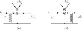
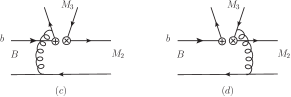
Figure 1: The emission diagrams with a vector meson emitted.

The factorizable emission diagrams are shown as the first two diagrams in Fig. 1. Since the tensor meson can not be generated from the vector or axial vector current, only the vector meson can be emitted. The expressions for all possible Lorentz structures are given as follows.

• (V-A)(V-A) factorizable emission diagrams:

  $$F_{vef}^{LL}(a_{i}) = 8\sqrt{\frac{2}{3}}\pi m_{B}^{4}f_{V}C_{F}\int_{0}^{1}dx_{1}dx_{2}\int_{0}^{1/\Lambda_{QCD}}b_{1}db_{1}b_{2}db_{2}\phi_{B}(x_{1})$$ (34)

  $$\left\{\left(r_{2}(2x_{2}-1)(\phi_{T}^{t}(x_{2})-\phi_{T}^{s}(x_{2}))+(2-x_{2})\phi_{T}(x_{2})\right)a_{i}(t_{vef}^{1})E_{e}(t_{vef}^{1})\right.$$

  $$\left.\times h_{e}(\sqrt{|\alpha_{ef1}^{2}|},\sqrt{|\beta_{ef1}^{2}|},b_{2},b_{1})S_{t}(x_{2})-2r_{2}\phi_{T}^{s}(x_{2})a_{i}(t_{vef}^{2})E_{e}(t_{vef}^{2})\right.$$

  $$\left.\times h_{e}(\sqrt{|\alpha_{ef2}^{2}|},\sqrt{|\beta_{ef2}^{2}|},b_{1},b_{2})S_{t}(x_{1})\right\}\;,$$

  where the explicit expressions of scales $t_{vef}^{1,2}$, the production of coupling $\alpha_{s}$ and Sudakov factor $E_{e}(t_{vef}^{1,2})$, the function of hard kernel $h_{e}$, the parameters $\alpha_{(ef1,ef2)}^{2}$ and $\beta_{(ef1,ef2)}^{2}$, and the jet function $S_{t}(x)$ are all collected in Appendix A. In the following analytic formulas, the expressions of all the additional functions can also be found in the same appendix.

• (V-A)(V+A) factorizable emission diagrams:

  $$F_{vef}^{LR}(a_{i})=F_{vef}^{LL}(a_{i})\;,$$ (35)

• (S-P)(S+P) factorizable emission diagrams:

  $$F_{vef}^{SP}(a_{i})=0\;.$$ (36)

Figure 2: The nonfactorizable emission diagrams with a tensor meson emitted.

There are two possible types of nonfactorizable emission diagrams, one has the vector meson emitted and the other has the tensor meson emitted. They are depicted by the last two diagrams of Fig. 1 and Fig. 2 respectively. We use the index $ten$ to represent the tensor meson emission and $ven$ for vector meson emission. The expressions are given by:

• (V-A)(V-A) nonfactorizable emission diagrams with vector meson emission:

  $$F_{ven}^{LL}(a_{i}) = \frac{32}{3}\pi m_{B}^{4}C_{F}\int_{0}^{1}dx_{1}dx_{2}dx_{3}\int_{0}^{1/\Lambda_{QCD}}b_{1}db_{1}b_{3}db_{3}\phi_{B}(x_{1})\phi_{V}(x_{3})$$ (37)

  $$\left\{\left(r_{2}(1-x_{2})(\phi_{T}^{s}(x_{2})+\phi_{T}^{t}(x_{2}))+x_{3}\phi_{T}(x_{2})\right)a_{i}(t_{ven}^{1})E_{en}(t_{ven}^{1},1,2)\right.$$

  $$\left.\times h_{en}(\sqrt{|\alpha_{en1}^{2}|},\sqrt{|\beta_{en1}^{2}|},b_{1},b_{3})+\left(r_{2}(x_{2}-1)(\phi_{T}^{s}(x_{2})-\phi_{T}^{t}(x_{2}))+(x_{2}+x_{3}-2)\phi_{T}(x_{2}))\right)\right.$$

  $$\left.\times a_{i}(t_{ven}^{2})E_{en}(t_{ven}^{2},1,2)h_{en}(\sqrt{|\alpha_{en2}^{2}|},\sqrt{|\beta_{en2}^{2}|},b_{1},b_{3})\right\}\;,$$

• (V-A)(V+A) nonfactorizable emission diagrams with vector meson emission:

  $$F_{ven}^{LR}(a_{i}) = \frac{32}{3}\pi m_{B}^{4}C_{F}r_{3}\int_{0}^{1}dx_{1}dx_{2}dx_{3}\int_{0}^{1/\Lambda_{QCD}}b_{1}db_{1}b_{3}db_{3}\phi_{B}(x_{1})$$ (38)

  $$\left\{\left(r_{2}((x_{2}-1)(\phi_{T}^{s}(x_{2})-\phi_{T}^{t}(x_{2}))(\phi_{V}^{s}(x_{3})+\phi_{V}^{t}(x_{3}))-x_{3}(\phi_{T}^{s}(x_{2})+\phi_{T}^{t}(x_{2}))(\phi_{V}^{s}(x_{3})-\phi_{V}^{t}(x_{3})))\right.\right.$$

  $$\left.\left.+x_{3}\phi_{T}(x_{2})(\phi_{V}^{s}(x_{3})-\phi_{V}^{t}(x_{3}))\right)a_{i}(t_{ven}^{1})E_{en}(t_{ven}^{1},1,2)h_{en}(\sqrt{|\alpha_{en1}^{2}|},\sqrt{|\beta_{en1}^{2}|},b_{1},b_{3})\right.$$

  $$\left.-\left(r_{2}(x_{2}(\phi_{V}^{s}(x_{3})-\phi_{V}^{t}(x_{3}))(\phi_{T}^{s}(x_{2})-\phi_{T}^{t}(x_{2}))+x_{3}(\phi_{V}^{s}(x_{3})+\phi_{V}^{t}(x_{3}))(\phi_{T}^{s}(x_{2})+\phi_{T}^{t}(x_{2}))\right.\right.$$

  $$\left.\left.-2(\phi_{V}^{s}(x_{3})\phi_{T}^{s}(x_{2})+\phi_{V}^{t}(x_{3})\phi_{T}^{t}(x_{2})))-(x_{3}-1)\phi_{T}(x_{2})(\phi_{V}^{s}(x_{3})+\phi_{V}^{t}(x_{3}))\right)\right.$$

  $$\left.\times a_{i}(t_{ven}^{2})E_{en}(t_{ven}^{2},1,2)h_{en}(\sqrt{|\alpha_{en2}^{2}|},\sqrt{|\beta_{en2}^{2}|},b_{1},b_{3})\right\}\;,$$

• (S-P)(S+P) nonfactorizable emission diagrams with vector meson emission:

  $$F_{ven}^{SP}(a_{i}) = \frac{32}{3}\pi m_{B}^{4}C_{F}\int_{0}^{1}dx_{1}dx_{2}dx_{3}\int_{0}^{1/\Lambda_{QCD}}b_{1}db_{1}b_{3}db_{3}\phi_{B}(x_{1})\phi_{V}(x_{3})$$ (39)

  $$\left\{\left(r_{2}(1-x_{2})(\phi_{T}^{s}(x_{2})-\phi_{T}^{t}(x_{2}))+\phi_{T}(x_{2})(-x_{2}+x_{3}+1)\right)a_{i}(t_{ven}^{1})E_{en}(t_{ven}^{1},1,2)\right.$$

  $$\left.\times h_{en}(\sqrt{|\alpha_{en1}^{2}|},\sqrt{|\beta_{en1}^{2}|},b_{1},b_{3})+\left(r_{2}(x_{2}-1)(\phi_{T}^{t}(x_{2})+\phi_{T}^{s}(x_{2}))+\phi_{T}(x_{2})(x_{3}-1)\right)a_{i}(t_{ven}^{2})\right.$$

  $$\left.\times E_{en}(t_{ven}^{2},1,2)h_{en}(\sqrt{|\alpha_{en2}^{2}|},\sqrt{|\beta_{en2}^{2}|},b_{1},b_{3})\right\}\;.$$

• (V-A)(V-A) nonfactorizable emission diagrams with tensor meson emission:

  $$F_{ten}^{LL}(a_{i}) = \frac{32}{3}\pi m_{B}^{4}C_{F}\int_{0}^{1}dx_{1}dx_{2}dx_{3}\int_{0}^{1/\Lambda_{QCD}}b_{1}db_{1}b_{2}db_{2}\phi_{B}(x_{1})\phi_{T}(x_{2})$$ (40)

  $$\left\{\left(x_{2}\phi_{V}(x_{3})-r_{3}(x_{3}-1)(\phi_{V}^{s}(x_{3})+\phi_{V}^{t}(x_{3}))\right)a_{i}(t_{ten}^{1})E_{en}(t_{ten}^{1},1,3)h_{en}(\sqrt{|\alpha_{en1}^{\prime 2}|},\sqrt{|\beta_{en1}^{\prime 2}|},b_{1},b_{2})\right.$$

  $$\left.+\left(r_{3}(x_{3}-1)(\phi_{V}^{s}(x_{3})-\phi_{V}^{t}(x_{3}))+\phi_{V}(x_{3})(x_{2}+x_{3}-2)\right)a_{i}(t_{ten}^{2})E_{en}(t_{ten}^{2},1,3)\right.$$

  $$\left.\times h_{en}(\sqrt{|\alpha_{en2}^{\prime 2}|},\sqrt{|\beta_{en2}^{\prime 2}|},b_{1},b_{2})\right\}\;,$$

• (V-A)(V+A) nonfactorizable emission diagrams with tensor meson emission:

  $$F_{ten}^{LR}(a_{i}) = \frac{32}{3}\pi m_{B}^{4}C_{F}r_{2}\int_{0}^{1}dx_{1}dx_{2}dx_{3}\int_{0}^{1/\Lambda_{QCD}}b_{1}db_{1}b_{2}db_{2}\phi_{B}(x_{1})$$ (41)

  $$\left\{\left(r_{3}(x_{2}(\phi_{V}^{s}(x_{3})+\phi_{V}^{t}(x_{3}))(\phi_{T}^{t}(x_{2})-\phi_{T}^{s}(x_{2}))+(1-x_{3})(\phi_{T}^{s}(x_{2})+\phi_{T}^{t}(x_{2}))(\phi_{V}^{t}(x_{3})-\phi_{V}^{s}(x_{3})))\right.\right.$$

  $$\left.\left.+x_{2}\phi_{V}(x_{3})(\phi_{T}^{s}(x_{2})-\phi_{T}^{t}(x_{2}))\right)a_{i}(t_{ten}^{1})E_{en}(t_{ten}^{1},1,3)h_{en}(\sqrt{|\alpha_{en1}^{\prime 2}|},\sqrt{|\beta_{en1}^{\prime 2}|},b_{1},b_{2})\right.$$

  $$\left.+\left(r_{3}(-x_{2}(\phi_{V}^{s}(x_{3})+\phi_{V}^{t}(x_{3}))(\phi_{T}^{s}(x_{2})+\phi_{T}^{t}(x_{2}))+x_{3}(\phi_{V}^{s}(x_{3})-\phi_{V}^{t}(x_{3}))(\phi_{T}^{t}(x_{2})-\phi_{T}^{s}(x_{2}))\right.\right.$$

  $$\left.\left.+2(\phi_{V}^{t}(x_{3})\phi_{T}^{t}(x_{2})+\phi_{V}^{s}(x_{3})\phi_{T}^{s}(x_{2})))+(x_{2}-1)\phi_{V}(x_{3})(\phi_{T}^{s}(x_{2})+\phi_{T}^{t}(x_{2}))\right)\right.$$

  $$\left.\times a_{i}(t_{ten}^{2})E_{en}(t_{ten}^{2},1,3)h_{en}(\sqrt{|\alpha_{en2}^{\prime 2}|},\sqrt{|\beta_{en2}^{\prime 2}|},b_{1},b_{2})\right\}\;,$$

• (S-P)(S+P) nonfactorizable emission diagrams with tensor meson emission:

  $$F_{ten}^{SP}(a_{i}) = \frac{32}{3}\pi m_{B}^{4}C_{F}\int_{0}^{1}dx_{1}dx_{2}dx_{3}\int_{0}^{1/\Lambda_{QCD}}b_{1}db_{1}b_{2}db_{2}\phi_{B}(x_{1})\phi_{T}(x_{2})$$ (42)

  $$\left\{\left(\phi_{V}(x_{3})(x_{2}-x_{3}+1)-r_{3}(x_{3}-1)(\phi_{V}^{s}(x_{3})-\phi_{V}^{t}(x_{3}))\right)a_{i}(t_{ten}^{1})E_{en}(t_{ten}^{1},1,3)\right.$$

  $$\left.\times h_{en}(\sqrt{|\alpha_{ef1}^{\prime 2}|},\sqrt{|\beta_{ef1}^{\prime 2}|},b_{1},b_{2})+\left(r_{3}(x_{3}-1)(\phi_{V}^{s}(x_{3})+\phi_{V}^{t}(x_{3}))+(x_{2}-1)\phi_{V}(x_{3})\right)a_{i}(t_{ten}^{2})\right.$$

  $$\left.\times E_{en}(t_{ten}^{2},1,3)h_{en}(\sqrt{|\alpha_{en2}^{\prime 2}|},\sqrt{|\beta_{en2}^{\prime 2}|},b_{1},b_{2})\right\}\;.$$

According to which meson has the anti-quark generated from the weak vertex, the annihilation diagrams are also divided into two types, as depicted in Figs. 3 and 4. We use the first letter of the index “$v$” to denote the case that the quark enters the vector meson and “$t$” to denote that the quark enters the tensor meson.

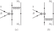
Figure 3: The annihilation diagrams with the electro-weak generated anti-quark entering the tensor meson.

Figure 4: The annihilation diagrams with the electro-weak generated anti-quark entering the vector meson.

For the factorizable annihilation diagrams, which are the first two diagrams in Figs. 3 and 4, the corresponding functions are given as follows.

• (V-A)(V-A) factorizable annihilation diagrams with the quark entering the vector meson:

  $$F_{vaf}^{LL}(a_{i}) = 8\sqrt{\frac{2}{3}}\pi m_{B}^{4}f_{B}C_{F}\int_{0}^{1}dx_{2}dx_{3}\int_{0}^{1/\Lambda_{QCD}}b_{2}db_{2}b_{3}db_{3}$$ (43)

  $$\left\{\left(-2r_{2}r_{3}\phi_{V}^{s}(x_{3})(-\phi_{T}^{s}(x_{2})(x_{2}+1)+\phi_{T}^{t}(x_{2})(1-x_{2}))-x_{2}\phi_{T}(x_{2})\phi_{V}(x_{3})\right)a_{i}(t_{vaf}^{1})\right.$$

  $$\left.\times E_{a}(t_{vaf}^{1})h_{a}(\sqrt{|\alpha_{af1}^{2}|},\sqrt{|\beta_{af1}^{2}|},b_{2},b_{3})S_{t}(x_{2})\right.$$

  $$\left.+\left(-2r_{2}r_{3}\phi_{T}^{s}(x_{2})((2-x_{3})\phi_{V}^{s}(x_{3})+x_{3}\phi_{V}^{t}(x_{3}))+(1-x_{3})\phi_{T}(x_{2})\phi_{V}(x_{3})\right)a_{i}(t_{vaf}^{2})\right.$$

  $$\left.\times E_{a}(t_{vaf}^{2})h_{a}(\sqrt{|\alpha_{af2}^{2}|},\sqrt{|\beta_{af2}^{2}|},b_{3},b_{2})S_{t}(x_{3})\right\}\;,$$

• (V-A)(V+A) factorizable annihilation diagrams with the quark entering the vector meson:

  $$F_{vaf}^{LR}(a_{i})=F_{vaf}^{LL}(a_{i})\;,$$ (44)

• (S-P)(S+P) factorizable annihilation diagrams with the quark entering the vector meson:

  $$F_{vaf}^{SP}(a_{i}) = 16\sqrt{\frac{2}{3}}\pi m_{B}^{4}f_{B}C_{F}\int_{0}^{1}dx_{2}dx_{3}\int_{0}^{1/\Lambda_{QCD}}b_{2}db_{2}b_{3}db_{3}$$ (45)

  $$\left\{\left(r_{2}x_{2}\phi_{V}(x_{3})(\phi_{T}^{t}(x_{2})-\phi_{T}^{s}(x_{2}))+2r_{3}\phi_{T}(x_{2})\phi_{V}^{s}(x_{3})\right)a_{i}(t_{vaf}^{1})E_{a}(t_{vaf}^{1})\right.$$

  $$\left.\times h_{a}(\sqrt{|\alpha_{af1}^{2}|},\sqrt{|\beta_{af1}^{2}|},b_{2},b_{3})S_{t}(x_{2})+\left(r_{3}(1-x_{3})\phi_{T}(x_{2})(\phi_{V}^{s}(x_{3})+\phi_{V}^{t}(x_{3}))-2r_{2}\phi_{T}^{s}(x_{2})\phi_{V}(x_{3})\right)\right.$$

  $$\left.\times a_{i}(t_{vaf}^{2})E_{a}(t_{vaf}^{2})h_{a}(\sqrt{|\alpha_{af2}^{2}|},\sqrt{|\beta_{af2}^{2}|},b_{3},b_{2})S_{t}(x_{3})\right\}\;.$$

• (V-A)(V-A) factorizable annihilation diagrams with the quark entering the tensor meson:

  $$F_{taf}^{LL}(a_{i}) = 8\sqrt{\frac{2}{3}}\pi m_{B}^{4}f_{B}C_{F}\int_{0}^{1}dx_{2}dx_{3}\int_{0}^{1/\Lambda_{QCD}}b_{2}db_{2}b_{3}db_{3}$$ (46)

  $$\left\{\left(2r_{2}r_{3}\phi_{T}^{s}(x_{2})((x_{3}+1)\phi_{V}^{s}(x_{3})+(x_{3}-1)\phi_{V}^{t}(x_{3}))-x_{3}\phi_{T}(x_{2})\phi_{V}(x_{3})\right)a_{i}(t_{taf}^{1})\right.$$

  $$\left.\times E_{a}(t_{taf}^{1})h_{a}(\sqrt{|\alpha_{af1}^{\prime 2}|},\sqrt{|\beta_{af1}^{\prime 2}|},b_{3},b_{2})S_{t}(x_{3})\right.$$

  $$\left.+\left(2r_{2}r_{3}\phi_{V}^{s}(x_{3})((x_{2}-2)\phi_{T}^{s}(x_{2})-x_{2}\phi_{T}^{t}(x_{2}))+(1-x_{2})\phi_{T}(x_{2})\phi_{V}(x_{3})\right)a_{i}(t_{taf}^{2})\right.$$

  $$\left.\times E_{a}(t_{taf}^{2})h_{a}(\sqrt{|\alpha_{af2}^{\prime 2}|},\sqrt{|\beta_{af2}^{\prime 2}|},b_{2},b_{3})S_{t}(x_{2})\right\}\;,$$

• (V-A)(V+A) factorizable annihilation diagrams with the quark entering the tensor meson:

  $$F_{taf}^{LR}(a_{i})=F_{taf}^{LL}(a_{i})\;,$$ (47)

• (S-P)(S+P) factorizable annihilation diagrams with the quark entering the tensor meson:

  $$F_{taf}^{SP}(a_{i}) = 16\sqrt{\frac{2}{3}}\pi m_{B}^{4}f_{B}C_{F}\int_{0}^{1}dx_{2}dx_{3}\int_{0}^{1/\Lambda_{QCD}}b_{2}db_{2}b_{3}db_{3}$$ (48)

  $$\left\{\left(r_{3}x_{3}\phi_{T}(x_{2})(\phi_{V}^{t}(x_{3})-\phi_{V}^{s}(x_{3}))+2r_{2}\phi_{T}^{s}(x_{2})\phi_{V}(x_{3})\right)a_{i}(t_{taf}^{1})E_{a}(t_{taf}^{1})\right.$$

  $$\left.\times h_{a}(\sqrt{|\alpha_{af1}^{\prime 2}|},\sqrt{|\beta_{af1}^{\prime 2}|},b_{3},b_{2})S_{t}(x_{3})+\left(r_{2}\phi_{V}(x_{3})(1-x_{2})(\phi_{T}^{s}(x_{2})+\phi_{T}^{t}(x_{2}))-2r_{3}\phi_{T}(x_{2})\phi_{V}^{s}(x_{3})\right)\right.$$

  $$\left.\times a_{i}(t_{taf}^{2})E_{a}(t_{taf}^{2})h_{a}(\sqrt{|\alpha_{af2}^{\prime 2}|},\sqrt{|\beta_{af2}^{\prime 2}|},b_{2},b_{3})S_{t}(x_{2})\right\}\;.$$

The nonfactorizable annihilation diagrams are depicted by the last two diagrams in Figs. 3 and 4, and their corresponding functions are given in the following.

• (V-A)(V-A) nonfactorizable annihilation diagrams with the quark entering the vector meson:

  $$F_{van}^{LL}(a_{i}) = \frac{32}{3}\pi m_{B}^{4}C_{F}\int_{0}^{1}dx_{1}dx_{2}dx_{3}\int_{0}^{1/\Lambda_{QCD}}b_{1}db_{1}b_{3}db_{3}\phi_{B}(x_{1})$$ (49)

  $$\left\{\left(r_{2}r_{3}\phi_{T}^{s}(x_{2})(\phi_{V}^{s}(x_{3})(x_{2}-x_{3}+3)+\phi_{V}^{t}(x_{3})(x_{2}+x_{3}-1))\right.\right.$$

  $$\left.\left.-r_{2}r_{3}\phi_{T}^{t}(x_{2})(\phi_{V}^{s}(x_{3})(x_{2}+x_{3}-1)+\phi_{V}^{t}(x_{3})(x_{2}-x_{3}-1))\right.\right.$$

  $$\left.\left.+(x_{3}-1)\phi_{T}(x_{2})\phi_{V}(x_{3})\right)a_{i}(t_{van}^{1})E_{an}(t_{van}^{1})h_{an}(\sqrt{|\alpha_{an1}^{2}|},\sqrt{|\beta_{an1}^{2}|},b_{2},b_{1})\right.$$

  $$\left.+\left(r_{2}r_{3}\phi_{T}^{s}(x_{2})(\phi_{V}^{s}(x_{3})(-x_{2}+x_{3}-1)+\phi_{V}^{t}(x_{3})(x_{2}+x_{3}-1))\right.\right.$$

  $$\left.\left.-r_{2}r_{3}\phi_{T}^{t}(x_{2})(\phi_{V}^{s}(x_{3})(x_{2}+x_{3}-1)+\phi_{V}^{t}(x_{3})(-x_{2}+x_{3}-1))\right.\right.$$

  $$\left.\left.+x_{2}\phi_{T}(x_{2})\phi_{V}(x_{3})\right)a_{i}(t_{van}^{2})E_{an}(t_{van}^{2})h_{an}(\sqrt{|\alpha_{an2}^{2}|},\sqrt{|\beta_{an2}^{2}|},b_{2},b_{1})\right\}\;,$$

• (V-A)(V+A) nonfactorizable annihilation diagrams with the quark entering the vector meson:

  $$F_{van}^{LR}(a_{i}) = \frac{32}{3}\pi m_{B}^{4}C_{F}\int_{0}^{1}dx_{1}dx_{2}dx_{3}\int_{0}^{1/\Lambda_{QCD}}b_{1}db_{1}b_{3}db_{3}\phi_{B}(x_{1})$$ (50)

  $$\left\{\left(r_{2}\phi_{V}(x_{3})(2-x_{2})(\phi_{T}^{s}(x_{2})+\phi_{T}^{t}(x_{2}))+r_{3}(x_{3}+1)\phi_{T}(x_{2})(\phi_{V}^{s}(x_{3})-\phi_{V}^{t}(x_{3}))\right)a_{i}(t_{van}^{1})\right.$$

  $$\left.\times E_{an}(t_{van}^{1})h_{an}(\sqrt{|\alpha_{an1}^{2}|},\sqrt{|\beta_{an1}^{2}|},b_{2},b_{1})\right.$$

  $$\left.+\left(r_{2}x_{2}\phi_{V}(x_{3})(\phi_{T}^{s}(x_{2})+\phi_{T}^{t}(x_{2}))+r_{3}(1-x_{3})\phi_{T}(x_{2})(\phi_{V}^{s}(x_{3})-\phi_{V}^{t}(x_{3}))\right)a_{i}(t_{van}^{2})\right.$$

  $$\left.\times E_{an}(t_{van}^{2})h_{an}(\sqrt{|\alpha_{an2}^{2}|},\sqrt{|\beta_{an2}^{2}|},b_{2},b_{1})\right\}\;,$$

• (S-P)(S+P) nonfactorizable annihilation diagrams with the quark entering the vector meson:

  $$F_{van}^{SP}(a_{i}) = \frac{32}{3}\pi m_{B}^{4}C_{F}\int_{0}^{1}dx_{1}dx_{2}dx_{3}\int_{0}^{1/\Lambda_{QCD}}b_{1}db_{1}b_{3}db_{3}\phi_{B}(x_{1})$$ (51)

  $$\left\{\left(r_{2}r_{3}\phi_{T}^{s}(x_{2})(\phi_{V}^{s}(x_{3})(x_{2}-x_{3}+3)-\phi_{V}^{t}(x_{3})(x_{2}+x_{3}-1))\right.\right.$$

  $$\left.\left.-r_{2}r_{3}\phi_{T}^{t}(x_{2})(\phi_{V}^{t}(x_{3})(x_{2}-x_{3}-1)-\phi_{V}^{s}(x_{3})(x_{2}+x_{3}-1))\right.\right.$$

  $$\left.\left.-x_{2}\phi_{T}(x_{2})\phi_{V}(x_{3})\right)a_{i}(t_{van}^{1})E_{an}(t_{van}^{1})h_{an}(\sqrt{|\alpha_{an1}^{2}|},\sqrt{|\beta_{an1}^{2}|},b_{2},b_{1})\right.$$

  $$\left.+\left(r_{2}r_{3}(-\phi_{T}^{s}(x_{2})(\phi_{V}^{s}(x_{3})(x_{2}-x_{3}+1)+\phi_{V}^{t}(x_{3})(x_{2}+x_{3}-1))\right.\right.$$

  $$\left.\left.+r_{2}r_{3}\phi_{T}^{t}(x_{2})(\phi_{V}^{t}(x_{3})(x_{2}-x_{3}+1)+\phi_{V}^{s}(x_{3})(x_{2}+x_{3}-1))\right.\right.$$

  $$\left.\left.-(x_{3}-1)\phi_{T}(x_{2})\phi_{V}(x_{3})\right)a_{i}(t_{van}^{2})E_{an}(t_{van}^{2})h_{an}(\sqrt{|\alpha_{an2}^{2}|},\sqrt{|\beta_{an2}^{2}|},b_{2},b_{1})\right\}\;.$$

• (V-A)(V-A) nonfactorizable annihilation diagrams with the quark entering the tensor meson:

  $$F_{tan}^{LL}(a_{i}) = \frac{32}{3}\pi m_{B}^{4}C_{F}\int_{0}^{1}dx_{1}dx_{2}dx_{3}\int_{0}^{1/\Lambda_{QCD}}b_{1}db_{1}b_{3}db_{3}\phi_{B}(x_{1})$$ (52)

  $$\left\{\left(r_{2}r_{3}\phi_{T}^{s}(x_{2})(\phi_{V}^{s}(x_{3})(-x_{2}+x_{3}+3)-\phi_{V}^{t}(x_{3})(x_{2}+x_{3}-1))\right.\right.$$

  $$\left.\left.+r_{2}r_{3}\phi_{T}^{t}(x_{2})(\phi_{V}^{s}(x_{3})(x_{2}+x_{3}-1)-\phi_{V}^{t}(x_{3})(-x_{2}+x_{3}-1))\right.\right.$$

  $$\left.\left.-(1-x_{2})\phi_{T}(x_{2})\phi_{V}(x_{3})\right)a_{i}(t_{van}^{1})E_{an}(t_{tan}^{1})h_{an}(\sqrt{|\alpha_{an1}^{\prime 2}|},\sqrt{|\beta_{an1}^{\prime 2}|},b_{2},b_{1})\right.$$

  $$\left.+\left(-r_{2}r_{3}\phi_{T}^{s}(x_{2})(\phi_{V}^{s}(x_{3})(-x_{2}+x_{3}+1)+\phi_{V}^{t}(x_{3})(x_{2}+x_{3}-1))\right.\right.$$

  $$\left.\left.+r_{2}r_{3}\phi_{T}^{t}(x_{2})(\phi_{V}^{s}(x_{3})(x_{2}+x_{3}-1)+\phi_{V}^{t}(x_{3})(-x_{2}+x_{3}+1))\right.\right.$$

  $$\left.\left.+x_{3}\phi_{T}(x_{2})\phi_{V}(x_{3})\right)a_{i}(t_{van}^{2})E_{an}(t_{tan}^{2})h_{an}(\sqrt{|\alpha_{an2}^{\prime 2}|},\sqrt{|\beta_{an2}^{\prime 2}|},b_{2},b_{1})\right\}\;,$$

• (V-A)(V+A) nonfactorizable annihilation diagrams with the quark entering the tensor meson:

  $$F_{tan}^{LR}(a_{i}) = \frac{32}{3}\pi m_{B}^{4}C_{F}\int_{0}^{1}dx_{1}dx_{2}dx_{3}\int_{0}^{1/\Lambda_{QCD}}b_{1}db_{1}b_{3}db_{3}\phi_{B}(x_{1})$$ (53)

  $$\left\{-\left(r_{2}\phi_{V}(x_{3})(x_{2}+1)(\phi_{T}^{t}(x_{2})-\phi_{T}^{s}(x_{2}))+r_{3}\phi_{T}(x_{2})(x_{3}-2)(\phi_{V}^{s}(x_{3})+\phi_{V}^{t}(x_{3}))\right)a_{i}(t_{van}^{1})\right.$$

  $$\left.\times E_{an}(t_{tan}^{1})h_{an}(\sqrt{|\alpha_{an1}^{\prime 2}|},\sqrt{|\beta_{an1}^{\prime 2}|},b_{2},b_{1})\right.$$

  $$\left.+\left(r_{3}x_{3}\phi_{T}(x_{2})(\phi_{V}^{s}(x_{3})+\phi_{V}^{t}(x_{3}))-r_{2}(1-x_{2})\phi_{V}(x_{3})(\phi_{T}^{t}(x_{2})-\phi_{T}^{s}(x_{2}))\right)a_{i}(t_{van}^{2})\right.$$

  $$\left.\times E_{an}(t_{tan}^{2})h_{an}(\sqrt{|\alpha_{an2}^{\prime 2}|},\sqrt{|\beta_{an2}^{\prime 2}|},b_{2},b_{1})\right\}\;,$$

• (S-P)(S+P) nonfactorizable annihilation diagrams with the quark entering the tensor meson:

  $$F_{tan}^{SP}(a_{i}) = \frac{32}{3}\pi m_{B}^{4}C_{F}\int_{0}^{1}dx_{1}dx_{2}dx_{3}\int_{0}^{1/\Lambda_{QCD}}b_{1}db_{1}b_{3}db_{3}\phi_{B}(x_{1})$$ (54)

  $$\left\{\left(r_{2}r_{3}\phi_{T}^{s}(x_{2})(\phi_{V}^{s}(x_{3})(-x_{2}+x_{3}+3)+\phi_{V}^{t}(x_{3})(x_{2}+x_{3}-1))\right.\right.$$

  $$\left.\left.-r_{2}r_{3}\phi_{T}^{t}(x_{2})(\phi_{V}^{s}(x_{3})(x_{2}+x_{3}-1)+\phi_{V}^{t}(x_{3})(-x_{2}+x_{3}-1))\right.\right.$$

  $$\left.\left.-x_{3}\phi_{T}(x_{2})\phi_{V}(x_{3})\right)a_{i}(t_{van}^{1})E_{an}(t_{tan}^{1})h_{an}(\sqrt{|\alpha_{an1}^{\prime 2}|},\sqrt{|\beta_{an1}^{\prime 2}|},b_{2},b_{1})\right.$$

  $$\left.+\left(-r_{2}r_{3}\phi_{T}^{s}(x_{2})(\phi_{V}^{s}(x_{3})(-x_{2}+x_{3}+1)-\phi_{V}^{t}(x_{3})(x_{2}+x_{3}-1))\right.\right.$$

  $$\left.\left.+r_{2}r_{3}\phi_{T}^{t}(x_{2})(\phi_{V}^{t}(x_{3})(-x_{2}+x_{3}+1)-\phi_{V}^{s}(x_{3})(x_{2}+x_{3}-1))\right.\right.$$

  $$\left.\left.-(x_{2}-1)\phi_{T}(x_{2})\phi_{V}(x_{3})\right)a_{i}(t_{van}^{2})E_{an}(t_{tan}^{2})h_{an}(\sqrt{|\alpha_{an2}^{\prime 2}|},\sqrt{|\beta_{an2}^{\prime 2}|},b_{2},b_{1})\right\}\;.$$

Similar to the $B\to VV$ decays, the amplitude of $B\to VT$ can be decomposed as

$${\cal A}(\epsilon_{2},\epsilon_{3}) = i{\cal A}^{N}+i(\epsilon^{*}_{T}\cdot\epsilon^{*}_{\bullet T}){\cal A}^{s}+(\epsilon_{\mu\nu\alpha\beta}n^{\mu}\bar{n}^{\nu}\epsilon^{*\alpha}_{T}\epsilon^{*\beta}_{\bullet T}){\cal A}^{p},$$ (55)

where ${\cal A}^{N}$ contains the contribution from the longitudinal polarizations, ${\cal A}^{s}$ and ${\cal A}^{p}$ represent the transversely polarized contributions. With the amplitude functions obtained in this section, the amplitude for the decay channels can be expressed. Considering the length of the paper, we will not list all the expressions of the amplitudes, but give one of the $B$ decay amplitude as an example:

$${\cal M}(B^{-}\to\rho^{-}a_{2}^{0})=\frac{G_{F}}{\sqrt{2}} \bigg{\{} V_{ub}V^{*}_{ud}[F^{LL}_{vef}(\frac{1}{\sqrt{2}}a_{1})+F^{LL}_{ven}(\frac{1}{\sqrt{2}}C_{1})+F^{LL}_{ten}(\frac{1}{\sqrt{2}}C_{2})+F^{LL}_{vaf}(\frac{1}{\sqrt{2}}a_{1})$$ (56)

$$+F^{LL}_{taf}(-\frac{1}{\sqrt{2}}a_{1})+F^{LL}_{van}(\frac{1}{\sqrt{2}}C_{1})+F^{LL}_{tan}(-\frac{1}{\sqrt{2}}C_{1})]-V_{tb}V^{*}_{td}[F^{LL}_{vef}(\frac{1}{\sqrt{2}}a_{4}+\frac{1}{\sqrt{2}}a_{10})$$

$$+F^{LL}_{ven}(\frac{1}{\sqrt{2}}C_{3}+\frac{1}{\sqrt{2}}C_{9})+F^{LL}_{ten}(-\frac{1}{\sqrt{2}}C_{3}+\frac{1}{2\sqrt{2}}C_{9}+\frac{3}{2\sqrt{2}}C_{10})$$

$$+F^{LR}_{ven}(\frac{1}{\sqrt{2}}C_{5}+\frac{1}{\sqrt{2}}C_{7})+F^{LR}_{ten}(-\frac{1}{\sqrt{2}}C_{5}+\frac{1}{2\sqrt{2}}C_{7})+F^{SP}_{vef}(\frac{1}{\sqrt{2}}a_{6}+\frac{1}{\sqrt{2}}a_{8})$$

$$+F^{SP}_{ten}(\frac{3}{2\sqrt{2}}C_{8})+F^{LL}_{vaf}(\frac{1}{\sqrt{2}}a_{4}+\frac{1}{\sqrt{2}}a_{10})+F^{LL}_{taf}(-\frac{1}{\sqrt{2}}a_{4}-\frac{1}{\sqrt{2}}a_{10})$$

$$+F^{LL}_{van}(\frac{1}{\sqrt{2}}C_{3}+\frac{1}{\sqrt{2}}C_{9})+F^{LL}_{tan}(-\frac{1}{\sqrt{2}}C_{3}-\frac{1}{\sqrt{2}}C_{9})+F^{LR}_{van}(\frac{1}{\sqrt{2}}C_{5}+\frac{1}{\sqrt{2}}C_{7})$$

$$+F^{LR}_{tan}(-\frac{1}{\sqrt{2}}C_{5}-\frac{1}{\sqrt{2}}C_{7})+F^{SP}_{vaf}(\frac{1}{\sqrt{2}}a_{6}+\frac{1}{\sqrt{2}}a_{8})+F^{SP}_{taf}(-\frac{1}{\sqrt{2}}a_{6}-\frac{1}{\sqrt{2}}a_{8})]\bigg{\}}.$$

3 Numerical results and discussions

With the amplitudes calculated in Sec. 2.3, the decay width is given as

$$\Gamma = \frac{[(1-(r_{2}+r_{3})^{2})(1-(r_{2}-r_{3})^{2})]^{1/2}}{16\pi m_{B}}\sum_{i}|A_{i}|^{2},$$ (57)

where $i$ represents all the polarization states, and the branching ratio is obtained through ${\cal BR}=\Gamma\tau_{B}$. The key observables of the decays related in this paper are the CP averaged branching ratios, polarization fractions, as well as direct CP asymmetries ($A_{\rm{CP}}^{\rm{dir}}$). Readers are referred to Ref. forcp for reviews on CP violation. First, we define four amplitudes as follows:

$$A_{f} = \langle f|{\cal H}|B\rangle,\;\;\;\bar{A}_{f}=\langle f|{\cal H}|\bar{B}\rangle,$$

$$A_{\bar{f}} = \langle\bar{f}|{\cal H}|B\rangle,\;\;\;\bar{A}_{\bar{f}}=\langle\bar{f}|{\cal H}|\bar{B}\rangle,$$ (58)

where $\bar{B}$ meson has a $b$ quark in it and $\bar{f}$ is the CP conjugate state of $f$. The direct CP asymmetry $A_{\rm{CP}}^{\rm{dir}}$ is defined by

$$A_{\rm{CP}}^{\rm{dir}} = \frac{|\bar{A}_{\bar{f}}|^{2}-|A_{f}|^{2}}{|\bar{A}_{\bar{f}}|^{2}+|A_{f}|^{2}}\;.$$ (59)

Our results for CP averaged branching ratios and CP asymmetries are listed in Tables 5, 6 and 7. In these tables, we also list the results of the longitudinal polarization fractions ${\cal R}_{L}$, which is defined by

$${\cal R}_{L} = \frac{|A_{0}|^{2}}{\sum_{i}|A_{i}|^{2}}\;,$$ (60)

where $A_{0}$ is the amplitude of the longitudinal polarization. The first error entries of our results are from the parameters in the wave functions, the decay constant $f_{B}$ and the shape parameter $\omega_{b}$. The second ones are from $\Lambda_{\rm{QCD}}$, which varies $20\%$ for error estimates, and from the scale $t$, which are listed in appendix A.

Table 3: The pQCD results for $B\to VT$ decays which have experimental data, where the experimental data is from the BaBar collaboration Amsler:2008zzb ; Aubert:2009sx ; Aubert:2008bc . Unit $10^{-6}$ for branching ratios, and $\%$ for the ${\cal R}_{L}$.

	$\cal BR$		${\cal R}_{L}$
Decay	This Work	Experiments	This Work	Experiments
$B^{-}\to K_{2}^{*}(1430)^{-}\omega$	$0.81^{+0.62+1.10}_{-0.54-0.62}$	$21.5\pm 4.3$	$47.0^{+0.8+0.3}_{-4.2-5.2}$	$56\pm 11$
$\bar{B}^{0}\to\bar{K}_{2}^{*}(1430)^{0}\omega$	$0.93^{+0.71+1.04}_{-0.51-0.73}$	$10.1\pm 2.3$	$55.6^{+3.1+3.0}_{-1.5-3.2}$	$45\pm 12$
$B^{-}\to K_{2}^{*}(1430)^{-}\phi$	$9.1^{+3.4+2.9}_{-2.6-2.0}$	$8.4\pm 2.1$	$82.1^{+6.2+8.7}_{-6.6-9.2}$	$80\pm 10$
$\bar{B}^{0}\to\bar{K}_{2}^{*}(1430)^{0}\phi$	$8.7^{+3.1+2.7}_{-2.5-1.9}$	$7.5\pm 1.0$	$82.0^{+6.5+8.1}_{-6.2-9.7}$	$90.1^{+5.9}_{-6.9}$

Table 4: The experimental branching ratios of $B\to K_{2}^{*}(1430)(\omega,\phi)$ decays Amsler:2008zzb ; Aubert:2009sx ; Aubert:2008bc and their corresponding $B\to VV$ decays Aubert:2008zza . The unit is $10^{-6}$.

Decays	$\cal BR$	Decays	$\cal BR$
$B^{-}\to K_{2}^{*}(1430)^{-}\omega$	$21.5\pm 4.3$	$B^{-}\to K^{*-}\omega$	$2.4\pm 1.0\pm 0.2$
$\bar{B}^{0}\to\bar{K}_{2}^{*}(1430)^{0}\omega$	$10.1\pm 2.3$	$\bar{B}^{0}\to\bar{K}^{*0}\omega$	$2.0\pm 0.5$
$B^{-}\to K_{2}^{*}(1430)^{-}\phi$	$8.4\pm 2.1$	$B^{-}\to K^{*-}\phi$	$10.0\pm 2.0$
$\bar{B}^{0}\to\bar{K}_{2}^{*}(1430)^{0}\phi$	$7.5\pm 1.0$	$\bar{B}^{0}\to\bar{K}^{*0}\phi$	$9.8\pm 0.6$

Before we go to the numerical discussions of Tables 5, 6 and 7, we note a few comments on the present experimental status. Only four channels, $B^{-}\to K_{2}^{*-}(\phi,\omega)$ and $\bar{B}^{0}\to K_{2}^{*0}(\phi,\omega)$, are reported by BaBar Amsler:2008zzb ; Aubert:2009sx ; Aubert:2008bc , which are shown in Tables 3 and 4. We also collect the corresponding decays in $B\to VV$ mode Aubert:2008zza for comparison. For the helicity structures of $B\to VT$ decays are very similar to the $B\to VV$ ones, a comparison between $B\to VT$ and $B\to VV$ would be very enlightening.

Comparing with the experimental data, one can see that the pQCD can give good predictions for the $B\to\phi(K_{2}^{*-},\bar{K}_{2}^{*0})$ decays. For the $B\to\omega(K_{2}^{*-},\bar{K}_{2}^{*0})$ decays, only the polarization fractions can be accommodated well, and large deviations exist in the branching ratios. Comparing our predictions with the experimental data, here we would like to make a few comments:

1. ${\cal BR}(B\to\phi(K_{2}^{*-},\bar{K}_{2}^{*0}))$ is very similar to ${\cal BR}(B\to\phi(K^{*-},\bar{K}^{*0}))$, but a little smaller, which might be understood easily by the effect of a heavier tensor mass on the phase space. It also indicates that only small effects are brought in the branching ratios when $K^{*}$ is substituted for $K_{2}^{*}$.

2. However, the experimental data shows totally opposite behavior for the $B\to\omega(K_{2}^{*-},\bar{K}_{2}^{*0},K^{*-},\bar{K}^{*0})$ decays, where ${\cal BR}(B\to\omega(K_{2}^{*-},\bar{K}_{2}^{*0}))$ is much larger than ${\cal BR}(B\to\omega(K^{*-},\bar{K}^{*0}))$. In the $B\to VV$ case, ${\cal BR}(B\to\phi(K^{*-},\bar{K}^{*0}))$ is about five times larger than ${\cal BR}(B\to\omega(K^{*-},\bar{K}^{*0}))$, while in the $B\to VT$ case ${\cal BR}(B\to\phi(K_{2}^{*-},\bar{K}_{2}^{*0}))$ is even smaller than ${\cal BR}(B\to\omega(K^{*-},\bar{K}^{*0}))$.

3. The pQCD predictions for the branching ratios of the $B\to VT$ decays are very similar to but a little smaller than the experimental data of $B\to VV$. Taking the errors into consideration, the similar numerical relationship between ${\cal BR}(B\to\phi(K^{*-},\bar{K}^{*0}))$ and ${\cal BR}(B\to\omega(K^{*-},\bar{K}^{*0}))$ mentioned above can also be accommodated in $B\to VT$ decays. As is well known, the $B\to VT$ decay is very similar to the $B\to VV$ decay mode theoretically, therefore the branching ratios in these two decay modes are expected to have the similar behavior. Based on such prejudice, the present experimental data is a little difficult to be understood.

4. However, only BaBar collaboration reported the results for $B\to\omega(K_{2}^{*-},\bar{K}_{2}^{*0})$ up to now, thus the experimental data need to be confirmed later. On the theoretical side, the tensor meson may bring forth new mechanism, which needs further investigations. In Ref. Cheng:2010yd the authors approached those channels in a different way. They used the experimental data of those channels to extract the penguin-annihilation parameters of the QCDF and predicted the other channels. By adopting the way, the experimental data could also be accommodated. However, we note more investigations are in need to understand the underlying dynamics totally.

Table 5: The branching ratios ($\cal{BR}$ in unit of $10^{-6}$), polarization fractions (${\cal R}_{L}$ in unit of $\%$) and direct CP violation ($A_{\rm{CP}}^{\rm{dir}}$ in unit of $\%$) of $B^{-}\to VT$ decays.

	$\cal{BR}$				${\cal{R}}_{L}$	$A_{\rm{CP}}^{\rm{dir}}$
	This Work	QCDFCheng:2010yd	ISGW2Kim:BtoVT	CLFJHMunoz:2009aba	This Work	This Work
$B^{-}\to\omega K_{2}^{*-}$	$0.81^{+0.62+1.10}_{-0.54-0.62}$	$7.5^{+19.7}_{-7.0}$	$0.112$	$0.06$	$47.0^{+0.8+0.3}_{-4.2-5.2}$	$-4.4_{-0.0-2.2}^{+0.4+3.7}$
$B^{-}\to\phi K_{2}^{*-}$	$9.1^{+3.4+2.9}_{-2.6-2.0}$	$7.4^{+25.8}_{-5.2}$	$2.180$	$9.24$	$82.1^{+6.2+8.7}_{-6.6-9.2}$	$1.5_{-0.1-0.3}^{+0.2+0.1}$
$B^{-}\to\rho^{-}a_{2}^{0}$	$12.8^{+7.1+2.4}_{-5.1-2.4}$	$8.4^{+4.7}_{-2.9}$	$7.432$	$19.34$	$93.4^{+0.8+1.2}_{-0.9-1.5}$	$6.5^{+1.4+1.6}_{-1.6-1.5}$
$B^{-}\to\rho^{-}\bar{K}_{2}^{*0}$	$3.9^{+1.2+1.8}_{-0.9-1.0}$	$18.6^{+50.1}_{-17.2}$			$57.6^{+1.6+1.8}_{-0.8-1.8}$	$0.43^{+0.50+0.56}_{-0.39-0.07}$
$B^{-}\to\rho^{0}a_{2}^{-}$	$0.67^{+0.30+0.37}_{-0.20-0.20}$	$0.82^{+2.30}_{-0.95}$	$0.007$	$0.071$	$50.8^{+5.1+9.5}_{-2.4-8.1}$	$-6.5^{+0.8+11.2}_{-0.4-7.9}$
$B^{-}\to\rho^{0}K_{2}^{*-}$	$2.3^{+0.6+0.8}_{-0.6-0.5}$	$10.4^{+18.8}_{-9.2}$	$0.253$	$0.74$	$67.6^{+2.2+1.9}_{-2.9-4.0}$	$-4.8^{+1.2+1.0}_{-1.8-0.9}$
$B^{-}\to\omega a_{2}^{-}$	$0.41^{+0.14+0.07}_{-0.14-0.06}$	$0.38^{+1.84}_{-0.36}$	$0.010$	$0.14$	$64.5^{+0.5+2.4}_{-2.8-5.1}$	$5.91^{+2.4+4.2}_{-6.9-7.0}$
$B^{-}\to\phi a_{2}^{-}$	$0.01^{+0.01+0.01}_{-0.00-0.00}$	$0.0003^{+0.013}_{-0.001}$	$0.004$	$0.019$	$67.4^{+0.8+4.3}_{-0.2-0.4}$	$--$
$B^{-}\to K^{*-}a_{2}^{0}$	$3.2^{+1.4+1.1}_{-0.9-0.6}$	$2.9^{+11.7}_{-2.5}$	$1.852$	$2.80$	$59.4^{+8.1+9.9}_{-7.9-10.7}$	$-4.1^{+2.9+5.8}_{-3.7-5.2}$
$B^{-}\to K^{*-}K_{2}^{*0}$	$0.39^{+0.09+0.15}_{-0.10-0.07}$	$2.1^{+4.2}_{-1.8}$			$68.1^{+0.0+5.3}_{-2.1-2.9}$	$-3.4^{+0.9+0.9}_{-1.6-5.1}$
$B^{-}\to K^{*0}K_{2}^{*-}$	$0.19^{+0.08+0.07}_{-0.06-0.05}$	$0.56^{+1.09}_{-0.38}$	$0.014$	$0.59$	$60.7^{+8.2+6.9}_{-8.8-9.8}$	$22.1^{+7.5+1.4}_{-7.7-5.2}$
$B^{-}\to\bar{K}^{*0}a_{2}^{-}$	$7.6^{+3.4+2.3}_{-2.7-1.9}$	$6.1^{+23.8}_{-5.4}$	$4.495$	$8.62$	$61.8^{7.3+8.9}_{-8.1-10.7}$	$-0.82^{+0.01+0.32}_{-0.25-0.27}$
$B^{-}\to\rho^{-}f_{2}$	$15.6^{+8.2+1.8}_{-6.1-2.2}$	$7.7^{+4.8}_{-2.9}$	$8.061$		$96.9^{+0.0+0.0}_{-0.0-0.0}$	$7.2^{+0.3+1.2}_{-0.6-1.3}$
$B^{-}\to\rho^{-}f_{2}^{\prime}$	$0.11^{+0.04+0.02}_{-0.03-0.02}$	$0.07^{+0.11}_{-0.04}$	$0.103$		$99.3^{+0.1+0.5}_{-0.0-0.8}$	$--$
$B^{-}\to K^{*-}f_{2}$	$7.3^{+2.8+2.4}_{-2.2-1.5}$	$8.3^{+17.3}_{-6.7}$	$2.032$		$76.3^{+4.1+1.2}_{-3.6-1.5}$	$-38.6^{+1.7+3.5}_{-0.7-2.7}$
$B^{-}\to K^{*-}f_{2}^{\prime}$	$1.7^{+0.5+1.0}_{-0.3-0.5}$	$12.6^{+24.0}_{-11.1}$	$0.025$		$15.1^{+4.2+5.1}_{-3.6-5.6}$	$-1.6^{+0.6+0.8}_{-1.0-1.2}$

Table 6: The branching ratios ($\cal{BR}$ in unit of $10^{-6}$), polarization fractions (${\cal R}_{L}$ in unit of $\%$) and direct CP violation ($A_{\rm{CP}}^{\rm{dir}}$ in unit of $\%$) of $\bar{B}_{d}^{0}\to VT$ decays.

	$\cal{BR}$				${\cal{R}}_{L}$	$A_{\rm{CP}}^{\rm{dir}}$
	This Work	QCDFCheng:2010yd	ISGW2Kim:BtoVT	CLFJHMunoz:2009aba	This Work	This Work
$\bar{B}_{d}^{0}\to\omega\bar{K}_{2}^{*0}$	$0.93^{+0.71+1.04}_{-0.51-0.73}$	$8.1^{+21.7}_{-7.6}$	$0.104$	$0.053$	$55.6^{+3.1+3.0}_{-1.5-3.2}$	$5.4_{-1.7-3.3}^{+1.9+3.5}$
$\bar{B}_{d}^{0}\to\phi\bar{K}_{2}^{*0}$	$8.7^{+3.1+2.7}_{-2.5-1.9}$	$7.7^{+26.9}_{-5.5}$	$2.024$	$8.51$	$82.0^{+6.5+8.1}_{-6.2-9.7}$	$--$
$\bar{B}_{d}^{0}\to\rho^{-}a_{2}^{+}$	$26.7^{+13.6+3.5}_{-10.2-3.9}$	$11.3^{+5.3}_{-4.6}$	$14.686$	$36.18$	$94.8^{+0.3+0.5}_{-0.3-0.6}$	$1.3^{+0.5+1.0}_{-0.4-0.9}$
$\bar{B}_{d}^{0}\to\rho^{+}a_{2}^{-}$	$0.74^{+0.19+0.16}_{-0.20-0.13}$	$1.2^{+2.6}_{-1.0}$			$88.7^{+0.8+1.3}_{-1.6-2.6}$	$7.7^{+3.2+0.6}_{-4.3-4.4}$
$\bar{B}_{d}^{0}\to\rho^{+}K_{2}^{*-}$	$3.4^{+1.1+1.6}_{-0.8-0.9}$	$19.8^{+52.0}_{-18.2}$			$53.9^{+1.0+1.3}_{-0.0-1.4}$	$-2.2^{+0.7+0.8}_{-0.9-0.8}$
$\bar{B}_{d}^{0}\to\rho^{0}a_{2}^{0}$	$0.68^{+0.30+0.22}_{-0.21-0.12}$	$0.39^{+1.35}_{-0.20}$	$0.003$	$0.03$	$90.7^{+1.0+1.5}_{-0.0-0.6}$	$13.6^{+2.1+5.3}_{-0.4-3.1}$
$\bar{B}_{d}^{0}\to\rho^{0}\bar{K}_{2}^{*0}$	$1.7^{+0.5+0.7}_{-0.4-0.4}$	$9.5^{+33.4}_{-9.5}$	$0.235$	$0.68$	$47.0^{+0.5+2.7}_{-0.8-1.7}$	$3.3^{+1.6+1.3}_{-1.1-1.9}$
$\bar{B}_{d}^{0}\to\omega a_{2}^{0}$	$0.37^{+0.11+0.0}_{-0.12-0.03}$	$0.25^{+1.14}_{-0.19}$	$0.005$	$0.07$	$89.5^{+0.3+1.2}_{-1.6-2.5}$	$5.7^{+8.9+11.1}_{-7.0-9.9}$
$\bar{B}_{d}^{0}\to\phi a_{2}^{0}$	$\sim 10^{-3}$	$0.001^{+0.006}_{-0.001}$	$0.002$	$0.009$	$45.0^{+1.5+4.8}_{-1.1-3.5}$	$--$
$\bar{B}_{d}^{0}\to K^{*-}a_{2}^{+}$	$6.1^{+2.8+2.1}_{-1.7-1.1}$	$6.1^{+24.3}_{-5.3}$	$3.477$	$7.25$	$59.3^{+8.3+9.1}_{-5.8-9.6}$	$-17.9^{+1.6+2.6}_{-4.4-4.9}$
$\bar{B}_{d}^{0}\to K^{*-}K_{2}^{*+}$	$3.0^{+0.7+1.4}_{-0.7-0.8}$	$0.43^{+0.54}_{-0.31}$			$49.8^{+0.3+0.3}_{-1.0-0.8}$	$5.9^{+3.7+4.3}_{-1.0-0.3}$
$\bar{B}_{d}^{0}\to K^{*+}K_{2}^{*-}$	$3.5^{+0.9+1.7}_{-0.8-0.9}$	$0.06^{+0.09}_{-0.03}$			$49.4^{+0.3+1.2}_{-0.6-0.4}$	$-1.2^{+0.4+1.6}_{-0.6-1.2}$
$\bar{B}_{d}^{0}\to K^{*0}\bar{K}_{2}^{*0}$	$4.5^{+1.3+2.2}_{-1.1-1.2}$	$0.44^{+0.88}_{-0.30}$	$0.026$	$0.55$	$40.6^{+1.9+2.7}_{-1.5-2.1}$	$6.1^{+1.4+1.3}_{-0.9-1.9}$
$\bar{B}_{d}^{0}\to\bar{K}^{*0}a_{2}^{0}$	$3.5^{+1.7+1.4}_{-1.2-0.8}$	$3.4^{+12.4}_{-2.8}$	$2.109$	$4.03$	$60.3^{+7.9+9.7}_{-7.7-9.9}$	$-11.1^{+0.2+2.2}_{-0.1-2.0}$
$\bar{B}_{d}^{0}\to\bar{K}^{*0}K_{2}^{*0}$	$5.1^{+1.4+2.3}_{-1.2-1.5}$	$1.1^{+2.9}_{-1.0}$			$55.1^{+0.7+0.0}_{-0.2-1.9}$	$0.41^{+0.22+0.31}_{-0.19-0.93}$
$\bar{B}_{d}^{0}\to\rho^{0}f_{2}$	$0.41^{+0.26+0.15}_{-0.16-0.07}$	$0.42^{+1.90}_{-0.44}$	$0.004$	$0.019$	$85.3^{+1.7+3.1}_{-1.1-2.0}$	$-1.9^{+0.0+5.2}_{-2.4-9.4}$
$\bar{B}_{d}^{0}\to\rho^{0}f_{2}^{\prime}$	$0.05^{+0.02+0.01}_{-0.01-0.01}$	$0.03^{+0.06}_{-0.02}$	$5\times 10^{-5}$		$99.3^{+0.0+0.4}_{-0.0-0.8}$	$--$
$\bar{B}_{d}^{0}\to\omega f_{2}$	$0.56^{+0.19+0.12}_{-0.16-0.11}$	$0.69^{+0.97}_{-0.36}$	$0.005$		$95.5^{+0.5+0.6}_{-0.5-0.9}$	$-5.7^{+5.9+7.5}_{-8.3-7.3}$
$\bar{B}_{d}^{0}\to\omega f_{2}^{\prime}$	$0.04^{+0.01+0.01}_{-0.01-0.01}$	$0.03^{+0.04}_{-0.01}$	$6\times 10^{-5}$		$99.2^{+0.0+0.0}_{-0.0-0.0}$	$--$
$\bar{B}_{d}^{0}\to\phi f_{2}$	$\sim 10^{-3}$	$0.001^{+0.007}_{-0.000}$	$0.002$		$73.0^{+1.12+5.53}_{-0.00-0.00}$	$--$
$\bar{B}_{d}^{0}\to\phi f_{2}^{\prime}$	$0.06^{+0.03+0.02}_{-0.01-0.05}$	$0.006^{+0.034}_{-0.005}$	$2\times 10^{-5}$		$10.0^{+33.1+24.6}_{-0.0-0.3}$	$0.67^{+0.0+0.59}_{-4.98-6.03}$
$\bar{B}_{d}^{0}\to\bar{K}^{*0}f_{2}$	$7.1^{+3.2+2.5}_{-2.1-1.3}$	$9.1^{+8.8}_{-7.3}$	$2.314$		$73.8^{+5.4+4.3}_{-3.3-1.4}$	$6.1^{+0.1+1.1}_{-0.4-1.2}$
$\bar{B}_{d}^{0}\to\bar{K}^{*0}f_{2}^{\prime}$	$1.8^{+0.6+1.1}_{-0.4-0.6}$	13.5${}^{+25.4}_{-11.9}$	$0.029$		$17.4^{+6.7+6.0}_{-1.5-2.5}$	$--$

We collect our results for $B_{u,d}\to VT$ decays in the Table 5 and 6, as well as the results of branching ratios under the QCDF and from the other two models. Most results of the pQCD and the QCDF agree with each other very well. For those channels, where the pQCD and the QCDF have obviously different central values, such as $B^{-}\to\rho^{-}\bar{K}_{2}^{*0}$ and $\bar{B}_{d}^{0}\to\rho^{+}\bar{K}_{2}^{*-}$, the penguin-annihilation parameters of the QCDF contribute the differences. The penguin-annihilation parameters are the key point of the QCDF to enhance the branching ratios of $B^{-}\to\omega\bar{K}_{2}^{*-}$ and $\bar{B}_{d}^{0}\to\omega\bar{K}_{2}^{*0}$ to accommodate the experimental data. We presume those parameters are the main factors for the large differences between the central values of these channels. However, taking the errors into consideration, the two different theoretical approaches can still agree with each other. On the other hand, future experimental observation of these channels may offer an opportunity to test the dynamics of the pQCD and the QCDF.

For the channels dominated by the $W$-emission diagrams, especially with a vector meson emitted, such as $\bar{B}_{d}^{0}\to a_{2}^{+}\rho^{-}$, the longitudinal contribution is dominating, and the polarization fraction ${\cal R}_{L}$ is around $90\%$. The polarization fractions of those decays dominated by the penguin diagrams are very profound. The polarization fractions of some penguin-dominating decays of $B\to VV$ decay mode like $B\to\phi K^{*0}$ are reported to be around $50\%$ Amsler:2008zzb , which are out of expectation of the SM. This is so-called the polarization puzzle in $B$ physics. However, one can find that the polarization fraction of $B\to\phi K_{2}^{*0}$ in the $B\to VT$ behaves as the SM expectation, while the $B\to\omega K_{2}^{*0}$ gives about $90\%$. In our calculation, we find that the polarization of $B\to VT$ for these channels are near to the $B\to VV$ ones. However, after we consider $r^{2}=(m_{T}/m_{B})^{2}$ contributions carefully, the polarizations can be accomodated to the experimental data, although the branching fractions cannot be accomodated.

From Eq. (59) one can see that the generation of the direct CP violation requires that the amplitude $A_{f}$ consists of at least two parts with different weak phases. Usually they are the tree contribution and penguin contributions in the SM. Readers are referred to Ref. Amsler:2008zzb for the related formulas and reviews. The interference of these parts will bring the direct CP violation. The magnitude of the direct CP violation is proportional to the ratio of the penguin and tree contributions. Therefore, the direct CP violation in the SM is very small, since the penguin contribution is almost always sub-dominating, which can be seen in previous section. However, there are a few very special channels in which the penguin contributions may be comparable to the tree one, as a result, sizeable direct CP violation appears. Take $B^{-}\to K^{*-}K_{2}^{*0}$ as an example. In this channel, the CKM matrix elements for the tree ($V_{ub}V^{*}_{ud}$) and penguin contributions ($V_{tb}V^{*}_{td}$) are at the same order. Although the Wilson coefficients for the tree contributions are much larger, the tree operator only appears in the annihilation diagrams, not in the emission ones. Therefore the tree contributions are suppressed, and the penguin ones become comparable, which brings to a relatively large direct CP violation for this channel.

Table 7: The branching ratios ($\cal{BR}$ in unit of $10^{-6}$), polarization fractions (${\cal R}_{L}$ in unit of $\%$) and direct CP violation ($A_{\rm{CP}}^{\rm{dir}}$ in unit of $\%$) of $\bar{B}_{s}^{0}\to VT$ decays.

	$\cal{BR}$	${\cal{R}}_{L}$	$A_{\rm{CP}}^{\rm{dir}}$
$\bar{B}_{s}^{0}\to\rho^{-}a_{2}^{+}$	$0.35^{+0.08+0.12}_{-0.11-0.08}$	$75.6^{+0.1+2.9}_{-1.5-3.4}$	$-11.0^{+3.7+4.9}_{-2.2-2.9}$
$\bar{B}_{s}^{0}\to\rho^{-}K_{2}^{*+}$	$17.1^{+7.7+1.2}_{-6.0-1.2}$	$93.5^{+0.2+0.5}_{-0.3-0.6}$	$4.2^{+0.7+0.8}_{-0.6-1.2}$
$\bar{B}_{s}^{0}\to\rho^{+}a_{2}^{-}$	$0.15^{+0.04+0.08}_{-0.04-0.05}$	$35.7^{+0.4+6.0}_{-1.2-3.3}$	$9.2^{+1.1+8.2}_{-1.3-7.6}$
$\bar{B}_{s}^{0}\to\rho^{0}a_{2}^{0}$	$0.03^{+0.01+0.02}_{-0.01-0.01}$	$99.1^{+0.3+0.6}_{-0.1-1.2}$	$-18.1^{+3.8+2.5}_{-1.3-5.2}$
$\bar{B}_{s}^{0}\to\rho^{0}K_{2}^{*0}$	$0.30^{+0.13+0.14}_{-0.10-0.08}$	$42.6^{+6.2+8.0}_{-5.9-8.5}$	$7.0^{+1.4+3.3}_{-2.0-4.7}$
$\bar{B}_{s}^{0}\to\omega a_{2}^{0}$	$\sim 10^{-3}$	$59.8^{+12.0+16.7}_{-5.6-13.3}$	$-18.8^{+1.7+12.7}_{-5.3-3.3}$
$\bar{B}_{s}^{0}\to\omega K_{2}^{*0}$	$0.13^{+0.05+0.07}_{-0.04-0.03}$	$49.6^{+2.6+6.3}_{-2.1-3.8}$	$-19.2^{+4.2+6.2}_{-4.8-4.2}$
$\bar{B}_{s}^{0}\to\phi a_{2}^{0}$	$0.04^{+0.01+0.005}_{-0.01-0.006}$	$99.2^{+0.1+0.3}_{-0.1-0.6}$	$-1.1^{+0.1+0.4}_{-1.1-2.2}$
$\bar{B}_{s}^{0}\to\phi K_{2}^{*0}$	$0.36^{+0.10+0.18}_{-0.09-0.10}$	$62.2^{+3.1+2.3}_{-0.9-0.9}$	$--$
$\bar{B}_{s}^{0}\to K^{*-}K_{2}^{*+}$	$4.5^{+1.6+1.7}_{-1.1-0.8}$	$39.9^{+7.8+11.3}_{-4.5-8.3}$	$-12.5^{+1.2+6.0}_{-0.6-4.3}$
$\bar{B}_{s}^{0}\to K^{*+}a_{2}^{-}$	$0.66^{+0.18+0.24}_{-0.17-0.15}$	$77.8^{+1.6+2.6}_{-0.7-3.2}$	$7.1^{+3.3+3.1}_{-3.0-3.0}$
$\bar{B}_{s}^{0}\to K^{*+}K_{2}^{*-}$	$6.1^{+1.5+2.5}_{-1.6-1.6}$	$59.9^{+0.3+0.7}_{-1.4-1.9}$	$-0.9^{+0.7+0.5}_{-0.6-0.4}$
$\bar{B}_{s}^{0}\to K^{*0}a_{2}^{0}$	$0.88^{+0.25+0.15}_{-0.23-0.13}$	$90.5^{+0.6+2.3}_{-0.6-3.1}$	$5.1^{+1.6+2.5}_{-2.6-3.5}$
$\bar{B}_{s}^{0}\to K^{*0}\bar{K}_{2}^{*0}$	$8.9^{+2.6+3.7}_{-2.2-2.1}$	$62.9^{+0.4+1.4}_{-1.6-2.9}$	$--$
$\bar{B}_{s}^{0}\to\bar{K}^{*0}K_{2}^{*0}$	$6.2^{+1.9+2.2}_{-1.7-1.5}$	$34.1^{+6.3+11.8}_{-5.2-12.2}$	$-4.2^{+0.2+0.8}_{-0.3-0.6}$
$\bar{B}_{s}^{0}\to\rho^{0}f_{2}$	$\sim 10^{-3}$	$69.5^{+1.8+8.1}_{-7.1-9.9}$	$-23.8^{+3.1+5.6}_{-1.6-3.8}$
$\bar{B}_{s}^{0}\to\rho^{0}f_{2}^{\prime}$	$0.12^{+0.05+0.01}_{-0.04-0.01}$	$89.8^{+0.0+0.4}_{-0.0-0.4}$	$14.2^{+0.8+2.1}_{-0.7-1.9}$
$\bar{B}_{s}^{0}\to\omega f_{2}$	$0.02^{+0.004+0.008}_{-0.003-0.009}$	$99.2^{+0.1+0.2}_{-0.3-1.0}$	$-13.9^{+2.6+2.4}_{-6.4-8.1}$
$\bar{B}_{s}^{0}\to\omega f_{2}^{\prime}$	$0.28^{+0.13+0.09}_{-0.10-0.06}$	$26.4^{+1.7+10.3}_{-0.4-7.4}$	$-1.3^{+0.5+1.6}_{-0.0-0.5}$
$\bar{B}_{s}^{0}\to\phi f_{2}$	$2.9^{+1.0+0.7}_{-0.9-0.7}$	$98.7^{+0.1+0.6}_{-0.0-1.1}$	$0.84^{+0.07+0.19}_{-0.35-0.41}$
$\bar{B}_{s}^{0}\to\phi f_{2}^{\prime}$	$3.1^{+1.8+0.6}_{-1.4-0.6}$	$75.3^{+3.0+3.5}_{-3.2-1.7}$	$--$
$\bar{B}_{s}^{0}\to K^{*0}f_{2}$	$0.51^{+0.17+0.11}_{-0.16-0.13}$	$92.2^{+1.6+2.4}_{-2.7-5.1}$	$-11.9^{+4.3+5.9}_{-2.5-2.4}$
$\bar{B}_{s}^{0}\to K^{*0}f_{2}^{\prime}$	$0.39^{+0.13+0.14}_{-0.09-0.08}$	$59.7^{+3.2+3.3}_{-2.2-3.1}$	$--$

For most of the $B\to VT$ decays, the pQCD predicts the branching ratios at the order of $10^{-6}$, which would be easy for the experimental observation. We also calculate the branching ratios, polarization fractions and the direct CP violations of $\bar{B}_{s}\to VT$ decays, which are collected in Table 7. Most of the $\bar{B}_{s}$ decays are penguin-dominated, whose branching ratios are mainly at the order of $10^{-7}$, therefore, whose observation requires more accumulation of experimental data. However, it would be easy for the forth-coming future flavor physics experiments. If a vector meson, generated by the tree operator whose decay constant is nonzero, is emitted in a $\bar{B}_{s}$ decay, then such channels have a large possibility to gain a relatively large branching ratios with the order of $10^{-6}$.

4 Summary

One of the valuable topics in flavor physics is studying the hadrons in the $B$ meson decays. In recent years, inspired by the interesting experimental data, more and more studies on the $B$ to tensor meson decays are carried on. The pQCD approach, which has been being developed for years and predicts many $B$ meson decays successfully, is a powerful tool in the study of two body non-leptonic $B$ meson decays. In this paper, we investigated the $B\to VT$ decays under the frame of the pQCD. We calculated all the tree level diagrams in the approach and collected all the necessary expressions in our paper, with which we can study the $39$ $B\to VT$ and $23$ $B_{s}\to VT$ decays. The branching ratios, polarization fractions, and direct CP violations are predicted.

Four channels in $B\to VT$ are reported by the experiments: $B\to\phi(K_{2}^{*-},\bar{K}_{2}^{*0})$ and $B\to\omega(K_{2}^{*-},\bar{K}_{2}^{*0})$. Comparing with their similar decays in the $B\to VV$ mode, these four channels have very interesting phenomena. On the experimental side, unlike the polarization puzzle in $B\to VV$ decays, the longitudinal polarization fractions of $B\to\phi(K_{2}^{*-},\bar{K}_{2}^{*0})$ decays are around $90\%$, while those of the $B\to\omega(K_{2}^{*-},\bar{K}_{2}^{*0})$ decays are around $50\%$. The branching ratios of $B\to\omega(K_{2}^{*-},\bar{K}_{2}^{*0})$ are much larger than those of $B\to\phi(K_{2}^{*-},\bar{K}_{2}^{*0})$. This is quite different from the $B\to VV$ case, where the branching ratio of $B\to\omega(K^{*-},\bar{K}^{*0})$ are about $5$ times larger than the ones of $B\to\phi(K^{*-},\bar{K}^{*0})$. By considering the $r^{2}=(m_{T}/m_{B})^{2}$ corrections, although the polarization fractions can be accommodated, the branching ratios are not predicted well. This may need further experimental confirmation and theoretical investigation.

Most of the branching ratios for $B^{-}$ and $\bar{B}^{0}$ decays are predicted to be at the order of $10^{-6}$. Most of our results agree with the the ones of the QCDF. Some channels do not agree so well by the central values, which may be caused by the different dynamics, since the QCDF introduce the penguin-annihilation parameters to accommodate the experimental data and their behavior seems different from the pQCD approach. However, taking the errors into consideration, they can still agree. For the decays which contributed by the $W$-emission diagram, especially when the vector meson is emitted, the polarization fraction is about $90\%$, which is just as the expectation of SM. The polarization fractions for the penguin dominated decays are complicated. Some are around $90\%$ and some are $50\%$, just like the cases of the four channels observed by the experiments. Fortunately, the main order of the $B^{-}$ and $\bar{B}^{0}$ decays is $10^{-6}$, which would be easy for the experimental observation.

In the $\bar{B}_{s}^{0}$ decays, the branching ratios are smaller. Such tree-dominated decays as $\bar{B}^{0}_{s}\to\rho^{-}K_{2}^{*+}$, when a vector meson is emitted, have the mechanism to gain a relatively large branching ratio at the order of $10^{-6}$. Most of the others are at the order of $10^{-7}$, whose observation need more accumulation of experimental data.

5 Acknowledgement

The work was supported by the National Research Foundation of Korea (NRF) grant funded by Korea government of the Ministry of Education, Science and Technology (MEST) (Grant No. 2011-0017430) and (Grant No. 2011-0020333). The work of Z.T.Z. was supported by the National Science Foundation of China under the Grant No.11075168, 11228512, and 11235005.

Appendix A Functions for hard kernel, Sudakov factors and scales

The parameters in the hard part is given as follows.

$$\beta^{2}_{ef1} = x_{1}(1-x_{2})m_{B}^{2}\,,\,\beta^{2}_{ef2}=\beta^{2}_{ef1}\,,$$

$$\alpha^{2}_{ef1} = (1-x_{2})m_{B}^{2}\,,\,\alpha_{ef2}^{2}=x_{1}m_{B}^{2}\,,$$

$$\beta^{2}_{en1} = (1-x_{2})(x_{1}-x_{3})m_{B}^{2}\,,\,\beta_{en2}^{2}=(1-x_{2})(x_{3}+x_{1}-1)m_{B}^{2}\,,$$

$$\alpha^{2}_{en1} = (1-x_{2})x_{1}m_{B}^{2}\,,\,\alpha_{en2}^{2}=\alpha^{2}_{en1}\,,$$

$$\beta^{2}_{af1} = -x_{2}(1-x_{3})m_{B}^{2}\,,\,\beta^{2}_{af2}=\beta^{2}_{af1}\,,$$

$$\alpha^{2}_{af1} = -x_{2}m_{B}^{2}\,,\,\alpha^{2}_{af2}=(x_{3}-1)m_{B}^{2}\,,$$

$$\beta^{2}_{an1} = [1-(x_{3}-x_{1})(1-x_{2})]m_{B}^{2}\,,\,\beta^{2}_{an2}=(x_{3}+x_{1}-1)x_{2}m_{B}^{2}\,,$$

$$\alpha^{2}_{an1} = -x_{2}(1-x_{3})m_{B}^{2}\,,\,\alpha^{2}_{an2}=\alpha^{2}_{an1}\,,$$

$$\beta^{\prime 2}_{i} = \beta^{2}_{i}(x_{2}\leftrightarrow x_{3})\,,\,\alpha^{\prime 2}_{i}=\alpha^{2}_{i}(x_{2}\leftrightarrow x_{3})\,,$$ (61)

where $i$ represents any indices.

The functions for the hard parts are given by

$$h_{e}(\alpha,\beta,b_{1},b_{2}) = K_{0}(\beta b_{2})[\theta(b_{2}-b_{1})I_{0}(b_{1}\alpha)K_{0}(b_{2}\alpha)+\theta(b_{1}-b_{2})I_{0}(b_{2}\alpha)K_{0}(b_{1}\alpha)],$$

$$h_{en}(\alpha,\beta,b_{1},b_{2}) = [\theta(b_{2}-b_{1})I_{0}(b_{1}\alpha)K_{0}(b_{2}\alpha)+\theta(b_{1}-b_{2})I_{0}(b_{2}\alpha)K_{0}(b_{1}\alpha)]\times\left\{\begin{array}[]{l}K_{0}(\beta b_{2})\,\,\,\,\,\,\mbox{for }\beta^{2}>0\\ \frac{i\pi}{2}H^{(1)}_{0}(\beta b_{2})\,\,\,\mbox{for }\beta^{2}<0\end{array}\right\},$$ (64)

$$h_{a}(\alpha,\beta,b_{1},b_{2}) = \left(\frac{i\pi}{2}\right)^{2}H_{0}^{(1)}(\beta b_{2})[\theta(b_{2}-b_{1})J_{0}(b_{1}\alpha)H^{(1)}_{0}(b_{2}\alpha)+\theta(b_{1}-b_{2})J_{0}(b_{2}\alpha)H^{(1)}_{0}(b_{1}\alpha)],$$

$$h_{an}(\alpha,\beta,b_{1},b_{2}) = \frac{i\pi}{2}[\theta(b_{2}-b_{1})J_{0}(b_{1}\alpha)H^{(1)}_{0}(b_{2}\alpha)$$ (67)

$$+\theta(b_{1}-b_{2})J_{0}(b_{2}\alpha)H^{(1)}_{0}(b_{1}\alpha)]\times\left\{\begin{array}[]{l}K_{0}(\beta b_{2})\,\,\,\,\,\,\mbox{for }\beta^{2}>0\\ \frac{i\pi}{2}H^{(1)}_{0}(\beta b_{2})\,\,\,\mbox{for }\beta^{2}<0\end{array}\right\},$$

where the $K_{0}$, $I_{0}$, $J_{0}$ and $H_{0}^{(1)}$ are all Bessel functions, and $H_{0}^{(1)}(z)=J_{0}(z)+iY_{0}(z)$.

The scales are defined as

$$t_{v..}^{l}=\max\left[c\sqrt{|\alpha_{..l}^{2}|},c\sqrt{|\beta_{..l}^{2}|},1/b_{k},1/b_{l}\right],\;t_{t..}^{l}=\max\left[c\sqrt{|\alpha_{..l}^{\prime 2}|},c\sqrt{|\beta_{..l}^{\prime 2}|},1/b_{k},1/b_{l}\right],$$ (68)

where $l=1,2$, the ”$..$” represents $ef$, $en$, $af$ or $an$, and $b_{k,l}$ represent the two corresponding $b$ coordinates in the measurement of the integration. The parameter $c=1$, and in our error estimation, we choose $c=0.75$ and $1.25$ for a rough estimation.

The expressions for the Sudakov factors and coupling constants are given as

$$E_{e}(t) = \alpha_{s}(t)\exp[-S_{B}(t)-S_{V}(t)]\;,$$

$$E_{a}(t) = \alpha_{s}(t)\exp[-S_{T}(t)-S_{V}(t)]\;,$$

$$E_{en}(t) = \left\{\begin{array}[]{l}\alpha_{s}(t)\exp[-S_{B}(t)-S_{T}(t)-S_{V}(t)|_{b_{2}=b_{1}}],\,\,\mbox{if vector meson emits}\\ \alpha_{s}(t)\exp[-S_{B}(t)-S_{T}(t)-S_{V}(t)|_{b_{3}=b_{1}}],\,\,\mbox{if tensor meson emits}\end{array}\right\}\;,$$ (71)

$$E_{an}(t) = \alpha_{s}(t)\exp[-S_{B}(t)-S_{T}(t)-S_{V}(t)|_{b_{3}=b_{2}}]\;,$$ (72)

where

$$S_{B}(t) = s(x_{1}\frac{m_{B}}{\sqrt{2}},b_{1})+\frac{5}{3}\int^{t}_{1/b_{1}}\frac{d\bar{\mu}}{\bar{\mu}}\gamma_{q}(\alpha_{s}(\bar{\mu})),$$

$$S_{T}(t) = s(x_{2}\frac{m_{B}}{\sqrt{2}},b_{2})+s((1-x_{2})\frac{m_{B}}{\sqrt{2}},b_{2})+2\int^{t}_{1/b_{2}}\frac{d\bar{\mu}}{\bar{\mu}}\gamma_{q}(\alpha_{s}(\bar{\mu})),$$

$$S_{V}(t) = s(x_{3}\frac{m_{B}}{\sqrt{2}},b_{3})+s((1-x_{3})\frac{m_{B}}{\sqrt{2}},b_{3})+2\int^{t}_{1/b_{3}}\frac{d\bar{\mu}}{\bar{\mu}}\gamma_{q}(\alpha_{s}(\bar{\mu})),$$ (73)

with the quark anomalous dimension $\gamma_{q}=-\alpha_{s}/\pi$. The explicit form for the function $s(Q,b)$ is:

$$s(Q,b) = ~{}~{}\frac{A^{(1)}}{2\beta_{1}}\hat{q}\ln\left(\frac{\hat{q}}{\hat{b}}\right)-\frac{A^{(1)}}{2\beta_{1}}\left(\hat{q}-\hat{b}\right)+\frac{A^{(2)}}{4\beta_{1}^{2}}\left(\frac{\hat{q}}{\hat{b}}-1\right)-\left[\frac{A^{(2)}}{4\beta_{1}^{2}}-\frac{A^{(1)}}{4\beta_{1}}\ln\left(\frac{e^{2\gamma_{E}-1}}{2}\right)\right]\ln\left(\frac{\hat{q}}{\hat{b}}\right)$$ (74)

$$+\frac{A^{(1)}\beta_{2}}{4\beta_{1}^{3}}\hat{q}\left[\frac{\ln(2\hat{q})+1}{\hat{q}}-\frac{\ln(2\hat{b})+1}{\hat{b}}\right]+\frac{A^{(1)}\beta_{2}}{8\beta_{1}^{3}}\left[\ln^{2}(2\hat{q})-\ln^{2}(2\hat{b})\right],$$

where the variables are defined by

$$\hat{q}\equiv\mbox{ln}[Q/(\sqrt{2}\Lambda)],~{}~{}~{}\hat{b}\equiv\mbox{ln}[1/(b\Lambda)],$$ (75)

and the coefficients $A^{(i)}$ and $\beta_{i}$ are

$$\beta_{1}=\frac{33-2n_{f}}{12},~{}~{}\beta_{2}=\frac{153-19n_{f}}{24},$$

$$A^{(1)}=\frac{4}{3},~{}~{}A^{(2)}=\frac{67}{9}-\frac{\pi^{2}}{3}-\frac{10}{27}n_{f}+\frac{8}{3}\beta_{1}\mbox{ln}(\frac{1}{2}e^{\gamma_{E}}),$$ (76)

$n_{f}$ is the number of the quark flavors and $\gamma_{E}$ is the Euler constant. We will use the one-loop running coupling constant, i.e. we pick up the four terms in the first line of the expression for the function $s(Q,b)$.

References

- (1) B. Aubert et al. [BABAR Collaboration], Phys. Rev. D 79, 052005 (2009) [arXiv:0901.3703 [hep-ex]].
- (2) B. Aubert et al. [BABAR Collaboration], Phys. Rev. Lett. 101, 161801 (2008) [arXiv:0806.4419 [hep-ex]].
- (3) B. Aubert et al. [BABAR Collaboration], Phys. Rev. D 78, 092008 (2008) [arXiv:0808.3586 [hep-ex]].
- (4) G. Lopez Castro and J. H. Munoz, Phys. Rev. D 55, 5581 (1997) [hep-ph/9702238].
- (5) J. H. Munoz, A. A. Rojas and G. Lopez Castro, Phys. Rev. D 59, 077504 (1999) [hep-ph/9812274].
- (6) C. S. Kim, B. H. Lim and S. Oh, Eur. Phys. J. C 22, 695 (2002) [Erratum-ibid. C 24, 665 (2002)] [hep-ph/0108054].
- (7) C.S. Kim, J.P. Lee, and S. Oh, Phys. Rev. D 67,014002(2003).
- (8) J H Munoz and N Quintero 2009 J. Phys. G: Nucl. Part. Phys. 36 095004.
- (9) A. Datta, Y. Gao, A. V. Gritsan, D. London, M. Nagashima and A. Szynkman, Phys. Rev. D 77, 114025 (2008) [arXiv:0711.2107 [hep-ph]].
- (10) H. -Y. Cheng and K. -C. Yang, Phys. Rev. D 83, 034001 (2011) [arXiv:1010.3309 [hep-ph]].
- (11) M. Beneke, G. Buchallla, M. Neubert, and C.T. Sachrajda, Phys. Rev. Lett. 83,1914 (1999); Nucl. Phys. B 591, 313 (2000); B 606, 245 (2001).
- (12) Y.Y. Keum, H.-n. Li, and A.I. Sanda, Phys. Rev. D 63, 054008 (2001).
- (13) C. Amsler et al. [Particle Data Group Collaboration], Phys. Lett. B 667, 1 (2008).
- (14) D.M. Li, H. Yu, and Q.X. Shen, J. Phys. G 27,807(2001).
- (15) H. -Y. Cheng, Y. Koike and K. -C. Yang, Phys. Rev. D 82, 054019 (2010) [arXiv:1007.3541 [hep-ph]].
- (16) W. Wang, Phys. Rev. D 83, 014008 (2011) [arXiv:1008.5326 [hep-ph]].
- (17) Z. -T. Zou, X. Yu and C. -D. Lu, arXiv:1203.4120 [hep-ph].
- (18) Z. -T. Zou, Z. Rui and C. -D. Lu, arXiv:1204.3144 [hep-ph].
- (19) Z. -T. Zou, X. Yu and C. -D. Lu, arXiv:1205.2971 [hep-ph].
- (20) Z. -T. Zou, X. Yu and C. -D. Lu, arXiv:1208.4252 [hep-ph].
- (21) S. Descotes-Genon and C. T. Sachrajda, Nucl. Phys. B 625, 239 (2002) [arXiv:hep-ph/0109260].
-
(22)
F. Feng, J. P. Ma and Q. Wang,
Phys. Lett. B 674, 176 (2009)
[arXiv:0807.0296 [hep-ph]];
H. n. Li and S. Mishima, Phys. Lett. B 674, 182 (2009) [arXiv:0808.1526 [hep-ph]];
F. Feng, J. P. Ma and Q. Wang, Phys. Lett. B 677, 121 (2009) [arXiv:0808.4017 [hep-ph]]. -
(23)
H. n. Li and S. Mishima,
Phys. Rev. D 71, 054025 (2005)
[arXiv:hep-ph/0411146];
H. n. Li, S. Mishima and A. I. Sanda, Phys. Rev. D 72, 114005 (2005) [arXiv:hep-ph/0508041];
H. n. Li and S. Mishima, Phys. Rev. D 74, 094020 (2006) [arXiv:hep-ph/0608277]. - (24) G. Buchalla, A. J. Buras and M. E. Lautenbacher, Rev. Mod. Phys. 68, 1125 (1996) [arXiv:hep-ph/9512380].
- (25) A. Ali, G. Kramer and C. D. Lu, Phys. Rev. D 58, 094009 (1998) [arXiv:hep-ph/9804363].
- (26) C. D. Lu and M. Z. Yang, Eur. Phys. J. C 28, 515 (2003) [arXiv:hep-ph/0212373].
- (27) M. Bauer and M. Wirbel, Z. Phys. C 42, 671 (1989).
- (28) Y.-Y. Keum, H.-n. Li and A. I. Sanda, Phys. Lett. B504, 6 (2001); Phys. Rev. D63, 054008 (2001); C.-D. Lü, K. Ukai and M.-Z. Yang, Phys. Rev. D63, 074009 (2001); C.-D. Lü and M.-Z. Yang, Eur. Phys. J. C23, 275-287 (2002);R. H. Li, C. D. Lu and H. Zou, Phys. Rev. D 78, 014018 (2008) [arXiv:0803.1073 [hep-ph]]; R. H. Li, X. X. Wang, A. I. Sanda and C. D. Lu, Phys. Rev. D 81, 034006 (2010) [arXiv:0910.1424 [hep-ph]].
- (29) A. Ali, G. Kramer, Y. Li, C. D. Lu, Y. L. Shen, W. Wang and Y. M. Wang, Phys. Rev. D 76, 074018 (2007) [arXiv:hep-ph/0703162].
- (30) P. Ball, G. W. Jones and R. Zwicky, Phys. Rev. D 75 (2007) 054004 [arXiv:hep-ph/0612081].
- (31) P. Ball and R. Zwicky, Phys. Lett. B 633, 289 (2006) [arXiv:hep-ph/0510338].
- (32) P. Ball and R. Zwicky, Phys. Rev. D 71, 014029 (2005); P. Ball and R. Zwicky, JHEP 0604, 046 (2006); P. Ball and G. W. Jones, JHEP 0703, 069 (2007).
- (33) T. M. Aliev and M. A. Shifman, Phys. Lett. B 112, 401 (1982).
- (34) T. M. Aliev and M. A. Shifman, Sov. J. Nucl. Phys. 36 (1982) 891 [Yad. Fiz. 36 (1982) 1532].
- (35) T. M. Aliev, K. Azizi and V. Bashiry, J. Phys. G 37, 025001 (2010) [arXiv:0909.2412 [hep-ph]].
- (36) P. Ball and V. M. Braun, Nucl. Phys. B 543, 201 (1999) [arXiv:hep-ph/9810475].
- (37) P. Ball, V. M. Braun, Y. Koike and K. Tanaka, Nucl. Phys. B 529, 323 (1998) [arXiv:hep-ph/9802299].
- (38) I.I.Y. Bigi and A.I. Sanda, Cambridge Monogr. Part. Phys., Nucl. Phys., Cosmol. 9, 1(2000); G.C. Branco, L. Lavoura, and J.P. Silva, CP Violation (Oxford University Press, Oxford, 1999).