Exact Classical Simulation
of the GHZ Distribution 

Abstract

John Bell has shown that the correlations entailed by quantum mechanics cannot be reproduced by a classical process involving non-communicating parties. But can they be simulated with the help of bounded communication? This problem has been studied for more than two decades and it is now well understood in the case of bipartite entanglement. However, the issue was still widely open for multipartite entanglement, even for the simplest case, which is the tripartite Greenberger–Horne–Zeilinger (GHZ) state. We give an exact simulation of arbitrary independent von Neumann measurements on general $n$-partite GHZ states. Our protocol requires $O(n^{2})$ bits of expected communication between the parties, and $O(n\log n)$ expected time is sufficient to carry it out in parallel. Furthermore, we need only an expectation of $O(n)$ independent unbiased random bits, with no need for the generation of continuous real random variables nor prior shared random variables. In the case of equatorial measurements, we improve on the prior art with a protocol that needs only $O(n\log n)$ bits of communication and $O(\log^{2}\!n)$ parallel time. At the cost of a slight increase in the number of bits communicated, these tasks can be accomplished with a constant expected number of rounds.

Keywords

Entanglement simulation, Greenberger–Horne–Zeilinger (GHZ) state, Multipartite entanglement, von Neumann’s rejection algorithm, Universal method of inversion, Knuth-Yao’s sampling algorithm.

1 Introduction

The issue of non-locality in quantum physics was raised in 1935 by Einstein, Podolsky and Rosen when they introduced the notion of entanglement [12]. Thirty years later, Bell proved that the correlations entailed by entanglement cannot be reproduced by classical local hidden variable theories between noncommunicating (e.g. space-like separated) parties [2]. This momentous discovery led to the question of quantifying quantum non-locality.

A natural quantitative approach to the non-locality inherent in a given entangled quantum state is to study the amount of resources that would be required in a purely classical theory to reproduce exactly the probabilities corresponding to measuring it. More formally, we consider the problem of sampling the joint discrete probability distribution of the outcomes obtained by people sharing this quantum state, on which each party applies locally some measurement on his share. Each party is given a description of his own measurement but not informed of the measurements assigned to the other parties. This task would be easy (for a theoretician!) if the parties were indeed given their share of the quantum state, but they are not. Instead, they must simulate the outcome of these measurements without any quantum resources, using as little classical communication as possible.

This conundrum was introduced by Maudlin [20] in 1992 in the simplest case of linear polarization measurements at arbitrary angles on the two photons that form a Bell state such as $|\Phi^{+}\rangle=\raisebox{0.17218pt}[0.0pt][0.0pt]{\small$\textstyle\frac{1}{\sqrt{2}}$}|00\rangle+\raisebox{0.17218pt}[0.0pt][0.0pt]{\small$\textstyle\frac{1}{\sqrt{2}}$}|11\rangle$. Maudlin claimed that this required “the capacity to send messages of unbounded length”, but he showed nevertheless that the task could be achieved with a bounded amount of expected communication. Similar concepts were reinvented independently years later by other researchers [5, 23]. This led to a series of results, culminating with the protocol of Toner and Bacon to simulate arbitrary von Neumann measurements on a Bell state with a single bit of communication in the worst case [24], thus contradicting Maudlin’s claim. Later, Regev and Toner extended this result by giving a simulation of the correlation (but not the marginals) entailed by arbitrary binary von Neumann measurements (meaning that the outcome for each party can take only two values) on arbitrary bipartite states of any dimension using only two bits of communication, also in the worst case [22]. Inspired by Steiner’s work [23], Cerf, Gisin and Massar showed that the effect of an arbitrary pair of positive-operator-valued measurements (POVMs) on a Bell state can also be simulated with a bounded amount of expected communication [9]. A more detailed early history of the simulation of quantum entanglement can be found in Ref. [4, Sect. 6].

All this prior work is concerned strictly with the simulation of bipartite entanglement. Much less is known when it comes to simulating multipartite entanglement with classical communication, a topic that was still teeming with major open problems. Consider the simplest case, which is the simulation of independent arbitrary von Neumann measurements on the tripartite GHZ state, named after Greenberger, Horne and Zeilinger [16], which we shall denote $|\Psi_{3}\rangle=\raisebox{0.17218pt}[0.0pt][0.0pt]{\small$\textstyle\frac{1}{\sqrt{2}}$}|000\rangle+\raisebox{0.17218pt}[0.0pt][0.0pt]{\small$\textstyle\frac{1}{\sqrt{2}}$}|111\rangle$, or more generally on its $n$-partite generalization $|\Psi_{n}\rangle=\raisebox{0.17218pt}[0.0pt][0.0pt]{\small$\textstyle\frac{1}{\sqrt{2}}$}|0^{n}\rangle+\raisebox{0.17218pt}[0.0pt][0.0pt]{\small$\textstyle\frac{1}{\sqrt{2}}$}|1^{n}\rangle$.

The easiest situation arises in the special case of equatorial measurements (defined in Section 2) on the GHZ state because all the marginal probability distributions obtained by tracing out one or more of the parties are uniform. Hence, it suffices in this case to simulate the $n$-partite correlation. Once this has been achieved, all the marginals can easily be made uniform [13]. Making the best of this observation, Bancal, Branciard and Gisin have given a protocol to simulate equatorial measurements on the tripartite and fourpartite GHZ states at an expected cost of 10 and 20 bits of communication, respectively [1]. Later on, Branciard and Gisin improved this in the tripartite case with a protocol using 3 bits of communication in the worst case [3]. The simulation of equatorial measurements on $|\Psi_{n}\rangle$ for $n\geq 5$ was handled subsequently by Brassard and Kaplan, with an expected cost of $O(n^{2})$ bits of communication [7]. This was the best result obtained until now on this line of work.

Despite substantial effort, the case of arbitrary von Neumann measurements, even on the original tripartite GHZ state $|\Psi_{3}\rangle$, was still wide open. Here, we solve this problem in the general case of the simulation of the $n$-partite GHZ state $|\Psi_{n}\rangle$, for any $n$, under the random bit model introduced in 1976 by Knuth and Yao [18], in which the only source of randomness comes from the availability of independently distributed unbiased random bits. Furthermore, we have no needs for prior shared random variables between the parties.  Our simulation proceeds with $O(n)$ expected perfect random bits and its expected communication cost is $O(n^{2})$ bits, but only $O(n\log n)$ time if we count one step for sending bits in parallel according to a realistic scenario in which no party has to send or receive more than one bit in any given step. Furthermore, in the case of equatorial measurements, we improve the earlier best result [7] with an expected communication cost of only $O(n\log n)$ bits and $O(\log^{2}\!n)$ parallel time. At the cost of a slight increase in the number of bits communicated and the number of required random bits, these tasks can be accomplished with a constant expected number of rounds.

More formally, the quantum task that we want to simulate is as follows. Each party $j$ holds one qubit (quantum bit) from state $|\Psi_{n}\rangle=\raisebox{0.17218pt}[0.0pt][0.0pt]{\small$\textstyle\frac{1}{\sqrt{2}}$}|0^{n}\rangle+\raisebox{0.17218pt}[0.0pt][0.0pt]{\small$\textstyle\frac{1}{\sqrt{2}}$}|1^{n}\rangle$ and is given the description of a von Neumann measurement $M_{j}$. By local operations, they collectively perform $\otimes_{j=1}^{n}M_{j}$ on $|\Psi_{n}\rangle$, thus obtaining one outcome each, say $b_{j}\in\{-1,+1\}$, which is their output. The joint probability distribution $p(b)$ of the $b_{j}$’s is defined by the joint set of measurements. Our purpose is to sample exactly this joint probability distribution by a purely classical process that involves no prior shared random variables and as little communication as possible. As mentioned above, previous solutions [1, 3, 7] required each individual measurement to be equatorial. In order to overcome this limitation, our complete solution builds on four ingredients: (1) Gravel’s decomposition of $p(b)$ as a convex combination of two sub-distributions [14, 15]; (2) Knuth and Yao’s algorithm [18] to sample exactly discrete probability distributions assuming only a source of unbiased identically independently distributed bits, rather than a source of continuous uniform random variables on the interval $[0,1]$; (3) the universal method of inversion [10, for instance]; and (4) our own distributed version of the classic von Neumann’s rejection algorithm [21].

We define precisely our problem in Section 2 and we formulate our convex decomposition of the GHZ distribution, which is the key to its simulation. Then, we explain how to sample according to a Bernoulli distribution even when only approximations of the distribution’s parameter are available. We also explain how the classic von Neumann rejection algorithm can be used to sample in the sub-distributions defined by our convex decomposition. However, little attention is paid in Section 2 to the fact that the various parameters that define the joint distribution are not available in a single place. Section 3 is concerned with the communication complexity issues. This paves the way to Section 4, in which we provide a complete protocol to solve our problem, as well as its detailed analysis. Section 5 discusses variations on the theme, in which we consider a parallel model of communication, an expected bounded-round solution, improvements on the prior art for the simulation of equatorial measurements, and a remark to the effect that only one party needs access to a source of randomness. We conclude in Section 6 with a discussion, open problems, and the announcement of a forthcoming generalization of our results to all multiparty entangled states in which each party is given a single qubit. For completeness, the appendices derive from first principles our convex decomposition of the GHZ distribution, as well as elementary approximation and truncation formulas useful in the analysis of the parallel model.

2 Sampling exactly the GHZ distribution in the random bit model

Any von Neumann measurement on a single qubit can be conveniently represented by a point on the surface of a three-dimensional sphere, known as the Bloch sphere, whose spherical coordinates can be specified by an azimuthal angle $\theta\in[0,2\pi)$ and an elevation angle $\varphi\in[-\pi/2,\pi/2]$. These parameters define operator

$$M=x\,\sigma_{1}+y\,\sigma_{2}+z\,\sigma_{3}=\left(\begin{array}[]{cc}\sin\varphi&e^{-\imath\theta}\,\cos\varphi\\ e^{\imath\theta}\,\cos\varphi&-\sin\varphi\end{array}\right)\,,$$

where $x=\cos\theta\cos\varphi$, $y=\sin\theta\cos\varphi$, $z=\sin\varphi$, and $\sigma_{1}$, $\sigma_{2}$ and $\sigma_{3}$ are the Pauli operators. In turn, this operator defines a measurement in the usual way, which we shall also call $M$ for convenience, whose outcome is one of its eigenvalues $+1$ or $-1$. The azimuthal angle $\theta$ represents the equatorial part of the measurement and the elevation angle $\varphi$ represents its real part. A von Neumann measurement is said to be equatorial when its elevation angle $\varphi=0$ vanishes and it is said to be in the computational basis when $\varphi=\pm\pi/2$.

Consider a set of $n$ von Neumann single-qubit measurements $M_{j}$, represented by their parameters $(\theta_{j},\varphi_{j})$, $1\leq j\leq n$. This set of operators defines a joint measurement $M=\otimes_{j=1}^{n}M_{j}$. In turn, this measurement defines a probability distribution $p$, which we shall call the GHZ distribution, on the set $\{-1,+1\}^{n}$. This distribution corresponds to the probability of all possible outcomes when the $n$-partite GHZ state $|\Psi_{n}\rangle=\raisebox{0.17218pt}[0.0pt][0.0pt]{\small$\textstyle\frac{1}{\sqrt{2}}$}|0^{n}\rangle+\raisebox{0.17218pt}[0.0pt][0.0pt]{\small$\textstyle\frac{1}{\sqrt{2}}$}|1^{n}\rangle$ is measured according to $M$.

Following Refs. [14, 15], we show in Appendix A that the probability $p(b)$ of obtaining $b=(b_{1},\ldots,b_{n})$ in $\{-1,+1\}^{n}$ can be decomposed as

$$\textstyle p(b)=\cos^{2}\!\big{(}\frac{\theta}{2}\big{)}\,p_{1}(b)+\sin^{2}\!\big{(}\frac{\theta}{2}\big{)}\,p_{2}(b)\,,\mbox{~{}where~{}}\mbox{$\theta=\sum_{j=1}^{n}\theta_{j}$}\mbox{~{}and}$$ (1)

$$p_{1}(b) =\frac{1}{2}\big{(}\mathrm{a}_{1}(b)+\mathrm{a}_{2}(b)\big{)}^{2}, p_{2}(b) =\frac{1}{2}\big{(}\mathrm{a}_{1}(b)-\mathrm{a}_{2}(b)\big{)}^{2},$$ (2)

$$\mathrm{a}_{1}(b) =\prod_{j=1}^{n}\textstyle{\cos\big{(}\frac{1}{2}\big{(}\varphi_{j}-\frac{\pi}{2}b_{j}\big{)}\big{)}}, \mathrm{a}_{2}(b) =\prod_{j=1}^{n}\textstyle{-\sin\big{(}\frac{1}{2}\big{(}\varphi_{j}-\frac{\pi}{2}b_{j}\big{)}\big{)}}\,.$$ (3)

Hence, we see that distribution $p$ is a convex combination of sub-distributions $p_{1}$ and $p_{2}$, in which the coefficients $\cos^{2}(\theta/2)$ and $\sin^{2}(\theta/2)$ depend only on the equatorial part of the measurements, whereas the sub-distributions depend only on their real part. Furthermore, it is easy to see that the squares of $\mathrm{a}_{1}$ and $\mathrm{a}_{2}$ are themselves discrete probability distributions.

Sampling $p$ is therefore a matter of sampling a Bernoulli distribution with defining parameter $\cos^{2}(\theta/2)$ before sampling either $p_{1}$ or $p_{2}$, whichever is the case. Notice that sampling $p_{2}$ reduces to sampling $p_{1}$ if, say, we replace $\varphi_{1}$ by $\varphi_{1}+2\pi$. As we shall see, full knowledge of the parameters is not required to sample $p$ exactly. We shall see in Section 2.1 how to sample a Bernoulli distribution with an arbitrary $p\in[0,1]$ as parameter (not the same $p$ as our probability distribution for GHZ) using a sequence of approximants converging to $p$ and using an expected number of only five unbiased identically independently distributed (i.i.d.) random bits. Subsequently, we shall see in Section 2.2 how to sample $p_{1}$ by modifying von Neumann’s rejection algorithm in a way that it uses sequences of approximants and unbiased i.i.d. random bits. For simulating exactly the GHZ distribution, an expected number of $6n+17$ perfect random bits is sufficient.

2.1 Sampling a Bernoulli distribution

Assume that only a random bit generator is available to sample a given probability distribution and that the parameters that specify this distribution are only accessible as follows: we can ask for any number of bits of each parameter, but will be charged one unit of cost per bit that is revealed. We shall also be charged for each random bit requested from the generator

To warm up to this conundrum, consider the problem of generating a Bernoulli random variable $Y$ with parameter $p\in[0,1]$. If $U=0.U_{1}U_{2}\ldots$ is the binary expansion of a uniform $[0,1]$ random variable, i.e. $U_{1},U_{2},\ldots$ is our source of unbiased independent random bits, and if $p=0.p_{1}p_{2}\ldots$ is the binary expansion of $p$ (in case $p=1$, we can proceed as if it were $0.p_{1}p_{2}\ldots$ with each $p_{i}=1$, and similarly for the probability $0$ event that $U=1$), we compare bits $U_{i}$ and $p_{i}$ for $i=1,2,\ldots$ until for the first time $U_{i}\not=p_{i}$. Then, if $U_{i}=0<p_{i}=1$, we return $Y=1$, and if $U_{i}=1>p_{i}=0$, we return $Y=0$. If we disregard the case $U=p$, which would result in an infinite loop but occurs with probability 0, it is clear that $Y=1$ if and only if $U<p$. Therefore, $Y$ is indeed Bernoulli$(p)$ since $U<p$ happens with probability $p$. The expected number of bits required from $p$ is precisely 2. The expected number of bits needed from our random bit source is also 2.

Now, suppose that the parameter $p$ defining our Bernoulli distribution is given by $p=\cos^{2}(\theta/2)$, as in the case of our decomposition of the GHZ distribution. None of the parties can know $\theta$ precisely since it is distributed as a sum of $\theta_{j}$’s, each of which is known only by one individual party. If we could obtain as many physical bits of $p$ as needed (although the expected number of required bits is as little as 2), we would use the idea given above in order to sample according to this Bernoulli distribution. However, it is not possible in general to know even the first bit of $p$ given any fixed number of bits of the $\theta_{j}$’s. (For instance, if $\theta$ is arbitrarily close to $\pi/2$, we need arbitrarily many bits of precision about it before we can tell if the first bit in the binary expansion of $\cos^{2}(\theta/2)$ is $0$ or $1$). Nevertheless, we can use approximations of $p$, rather than truncations, which in turn can come from approximations (in particular truncations) of the $\theta_{j}$’s.

Definition 1.

A $k$-bit approximation of a real number $x$ is any $\hat{x}$ such that $|x-\hat{x}|\leq 2^{-k}$. A special case of $k$-bit approximation is the $k$-bit truncation $\hat{x}=\mathrm{sign}(x)\lfloor|x|2^{k}\rfloor/2^{k}$, where $\mathrm{sign}(x)$ is equal to $+1$, $0$ or $-1$ depending on the sign of $x$. Note that the value of $k$ corresponds to the number of bits in the fractional part, without limitation on the size of the integer part, and that it does not take account of the sign in case it has to be transmitted too.

Algorithm 1 Sampling a Bernoulli random variable with approximate defining parameter

1:  Set $k\leftarrow 1$

2:  Set $U[0]\leftarrow 0$

3:  loop

4:     Generate an i.i.d. unbiased bit $U_{k}$

5:     Compute $U[k]\leftarrow U[k-1]+U_{k}/2^{k}$ {hence $U[k]=0.U_{1}\ldots U_{k}$}

6:     Obtain $p[k]$ so that $|p[k]-p|\leq 1/2^{k}$

7:     if $U[k]\leq p[k]-2/2^{k}$ then

8:        return $Y=1$

9:     else if $U[k]\geq p[k]+1/2^{k}$ then

10:        return $Y=0$

11:     else

12:        $k\leftarrow k+1$

13:     end if

14:  end loop

We postpone to Section 3.2 the detail of how these approximations can be obtained in a distributed setting. For the moment, assume that we can obtain $p[k]$ so that $|p[k]-p|\leq 1/2^{k}$ for any $k$. Then, setting $U[k]=0.U_{1}\ldots U_{k}$, we have that $U\leq p$ if $U[k]\leq p[k]-2/2^{k}$ whereas $U\geq p$ if $U[k]\geq p[k]+1/2^{k}$. Thus, one can check if $U<p$ (again disregarding the probability $0$ event that $U=p$) by generating only as many bits of $U$ and increasingly good approximations of $p$ as needed. These ideas are formalized in Algorithm 1 (on page 1). It is elementary to verify that the $Y$ generated by this algorithm is Bernoulli$(p)$, again because $\mathbf{P}\{U<p\}=p$ if $U$ is a continuous uniform random variable on $[0,1]$.

The number of iterations before Algorithm 1 returns a value, which is also its required number of independent unbiased random bits, is a random variable, say $K$. We have seen above that $\mathbf{E}\{K\}$, the expected value of $K$, would be exactly 2 if we could generate arbitrarily precise truncations of $p$. But since we can only obtain arbitrarily precise approximations instead, which is why we needed Algorithm 1 in the first place, we shall have to pay the price of a small increase in $\mathbf{E}\{K\}$.

$$\mathbf{P}\{K>k\}\leq\mathbf{P}\left\{|U[k]-p[k]|\leq\frac{2}{2^{k}}\right\}\leq\mathbf{P}\left\{|U-p|\leq\frac{4}{2^{k}}\right\}\leq\frac{8}{2^{k}}.$$

Therefore,

$$\mathbf{E}\{K\}=\sum_{k=0}^{\infty}\mathbf{P}\{K>k\}\leq\sum_{k=0}^{\infty}\min\left(1,\frac{8}{2^{k}}\right)=5.$$

2.2 Sampling $p_{1}$ (or $p_{2}$) in the random bit model

As mentioned already, it suffices to concentrate on $p_{1}$ since one can sample $p_{2}$ in exactly the same way provided one of the angles $\varphi_{j}$ is replaced by $\varphi_{j}+2\pi$: this introduces the required minus sign in front of $\mathrm{a}_{2}$ to transform $p_{1}$ into $p_{2}$. Let us define

$$\textstyle\alpha_{j}=\cos\!\big{(}\frac{1}{2}\big{(}\varphi_{j}-\frac{\pi}{2}\big{)}\big{)}=\sin\!\big{(}\frac{1}{2}\big{(}\varphi_{j}+\frac{\pi}{2}\big{)}\big{)}\mbox{~{}~{}~{}and~{}~{}~{}}\beta_{j}=\cos\!\big{(}\frac{1}{2}\big{(}\varphi_{j}+\frac{\pi}{2}\big{)}\big{)}=-\sin\!\big{(}\frac{1}{2}\big{(}\varphi_{j}-\frac{\pi}{2}\big{)}\big{)}\,.$$ (4)

Clearly, $\alpha_{j}^{2}+\beta_{j}^{2}=1$. Now, consider $n$ Rademacher  random variables $B_{j}$ that take value $-1$ with probability $\beta_{j}^{2}$ and $+1$ with complementary probability $\alpha_{j}^{2}$. The random vector with independent components given by $(B_{1},\ldots,B_{n})$ is distributed according to

$$q_{1}(b)\stackrel{{\scriptstyle\textrm{def}}}{{=}}\prod_{j\in F_{b}}\beta_{j}^{2}\prod_{j\in G_{b}}\alpha_{j}^{2}\,,$$

where $F_{b}=\{j\mid b_{j}=-1\}$ and $G_{b}=\{j\mid b_{j}=+1\}$ for all $b=(b_{1},\ldots,b_{n})\in\{-1,+1\}^{n}$. It is easy to verify that $q_{1}(b)=\mathrm{a}_{1}^{2}(b)$ for all $b$, where $\mathrm{a}_{1}$ is given in Equation (3). Similarly, the random vector with independent components given by $(-B_{1},\ldots,-B_{n})$ is distributed according to

$$q_{2}(b)\stackrel{{\scriptstyle\textrm{def}}}{{=}}\prod_{j\in F_{b}}\alpha_{j}^{2}\prod_{j\in G_{b}}\beta_{j}^{2}=\mathrm{a}_{2}^{2}(b)\,.$$

The key observation is that both $q_{1}$ and $q_{2}$ can be sampled without any needs for communication because each party $j$ knows his own parameters $\alpha_{j}^{2}$ and $\beta_{j}^{2}$, which is sufficient to draw independently according to local Rademacher random variable $B_{j}$ or $-B_{j}$. Moreover, a single unbiased independent random bit $S$ drawn by a designated party suffices to sample collectively from distribution $q=\frac{q_{1}+q_{2}}{2}$, provided this bit is transmitted to all parties: everybody samples according to $q_{1}$ if $S=0$ or to $q_{2}$ if $S=1$. Now, It follows from Equation (2) that $p_{1}(b)+p_{2}(b)=\mathrm{a}_{1}^{2}(b)+\mathrm{a}_{2}^{2}(b)=q_{1}(b)+q_{2}(b)$ for all $b\in\{-1,+1\}^{n}$, and therefore $p_{1}(b)\leq q_{1}(b)+q_{2}(b)=2q(b)$.

The relevance of all these observations is that we can apply von Neumann’s rejection algorithm [21] to sample $p_{1}$ since it is bounded by a small constant (2) times an easy-to-draw probability distribution ($q$). For the moment, we assume once again the availability of a continuous uniform random generator, which we shall later replace by a source of unbiased independent random bits. We also assume for the moment that we can compute the $\alpha_{j}$’s, $p_{1}(b)$, $q_{1}(b)$ and $q_{2}(b)$ exactly. This gives rise to Algorithm 2.

Algorithm 2 Sampling $p_{1}$ using von Neumann’s rejection algorithm

1:  repeat

2:     Generate $U$ uniformly on $[0,1]$

3:     Generate independent Rademacher random variables $B_{1},\ldots,B_{n}$ with parameters $\alpha_{1}^{2},\ldots,\alpha_{n}^{2}$

4:     Generate an unbiased independent random bit $S$

5:     if  $S=1$  then

6:        set $B\leftarrow(B_{1},\ldots,B_{n})$

7:     else

8:        set $B\leftarrow(-B_{1},\ldots,-B_{n})$

9:     end if

10:  until  $U\,(q_{1}(B)+q_{2}(B))\leq p_{1}(B)$

By the general principle of von Neumann’s rejection algorithm, probability distribution $p_{1}$ is successfully sampled after an expected number of 2 iterations round the loop because $p_{1}(b)\leq 2q(b)$ for all $b\in\{-1,+1\}^{n}$. Within one iteration, 2 expected independent unbiased random bits suffice to generate each of the $n$ Rademacher random variables by a process similar to what is explained in the second paragraph of Section 2.1. Hence an expected total of $2n+1$ random bits are needed each time round the loop for an expected grand total of $4n+2$ bits to sample $p_{1}$. But of course, this does not take account of the (apparent) need to generate the continuous uniform $[0,1]$ random variable $U$. It follows that the expected total amount of work required by Algorithm 2 is $O(n)$, provided we count infinite real arithmetic at unit cost. Furthermore, the time taken by this algorithm, divided by $n$, is stochastically smaller than a geometric random variable with constant mean, so its tail is exponentially decreasing.

Now, we modify and adapt this algorithm to eliminate the need for the continuous uniform $U$ (and hence its generation), which is not allowed in the random bit model. Furthermore, we eliminate the need for infinite real arithmetic and for the exact values of $q_{1}(B)$, $q_{2}(B)$ and $p_{1}(B)$, which would be impossible to obtain in our distributed setting since the parameters needed to compute these values are scattered among all parties, and replace them with approximations—we postpone to Section 3 the issue of how these approximations can be computed. (On the other hand, arbitrarily precise values of the $\alpha_{j}$’s are available to generate independent Rademacher random variables with these parameters because each party will be individually responsible to generate his own Rademacher.)

In each iteration of Algorithm 2, we generated a pair $(U,B)$. However, we did not really need $U$: we merely needed to generate a Bernoulli random variable $Y$ for which

$$\mathbf{P}\{Y=1\}=\mathbf{P}\left\{U\,(q_{1}(B)+q_{2}(B))\leq p_{1}(B)\right\}.$$

For this, we adapt the method developed for Algorithm 1. Again, we denote by $U[k]$ the $k$-bit truncation of $U$, so that $U[k]\leq U\leq U[k]+2^{-k}$. Furthermore, we use $L_{k}$ ($L$ for left) and $R_{k}$ ($R$ for right) to denote $k$-bit approximations of $q_{1}(B)+q_{2}(B)$ and $p_{1}(B)$, respectively, so that $|L_{k}-\big{(}q_{1}(B)+q_{2}(B)\big{)}|\leq 2^{-k}$ and $|R_{k}-p_{1}(B)|\leq 2^{-k}$. Then, we use $\varepsilon_{k}$ to denote the real number in interval $[-1,1]$ so that

$$|U[k]L_{k}-U\,(q_{1}(B)+q_{2}(B))| = \Big{|}U[k]L_{k}-U\,\Big{(}L_{k}+\frac{\varepsilon_{k}}{2^{k}}\Big{)}\Big{|}$$

$$= \Big{|}(U[k]-U)L_{k}-\frac{U\varepsilon_{k}}{2^{k}}\Big{|}~{}\leq~{}\frac{L_{k}}{2^{k}}+\frac{1}{2^{k}}~{}\leq~{}\frac{3}{2^{k}}\,.$$

Furthermore, because $R_{k}$ is a $k$-bit approximation of $p_{1}(B)$,

$$|R_{k}-p_{1}(B)|\leq\frac{1}{2^{k}}\,.$$

Thus, we know that $Y=1$ whenever

$$U[k]L_{k}+3/2^{k}<R_{k}-1/2^{k}\,,$$

whereas $Y=0$ whenever

$$U[k]L_{k}-3/2^{k}>R_{k}+1/2^{k}\,.$$

Otherwise, we are in the uncertainty zone and we need more bits of $U$, $q_{1}(B)+q_{2}(B)$ and $p_{1}(B)$ before we can decide on the value of $Y\!$. This is formalized in Algorithm 3.

Algorithm 3 Generator for the stopping condition in Algorithm 2

1:  Note: $B\in\{-1,+1\}^{n}$ is given to the algorithm, generated according to $\frac{q_{1}+q_{2}}{2}$

2:  Set $k\leftarrow 1$

3:  Set $U[0]\leftarrow 0$

4:  loop

5:     Generate an i.i.d. unbiased bit $U_{k}$

6:     Compute $U[k]\leftarrow U[k-1]+U_{k}/2^{k}$ {hence $U[k]=0.U_{1}\ldots U_{k}$}

7:      Compute $L_{k}$ and $R_{k}$ from $B$

8:     if $U[k]\,L_{k}-R_{k}<-\frac{4}{2^{k}}$ then

9:        return $Y=1$

10:     else if $U[k]\,L_{k}-R_{k}>\frac{4}{2^{k}}$ then

11:        return $Y=0$

12:     else

13:        $k\leftarrow k+1$

14:     end if

15:  end loop

It follows from the above discussion that this algorithm can be used to sample random variable $Y\!$, which is used as terminating condition in Algorithm 2, in order to eliminate the need for the generation of a continuous uniform random variable $U\in[0,1]$ and for the precise values of $q_{1}(B)$, $q_{2}(B)$ and $p_{1}(B)$. Since $L_{k}\to q_{1}(B)+q_{2}(B)$ and $R_{k}\to p_{1}(B)$ as $k\rightarrow\infty$, Algorithm 3 halts with probability 1. Let $K$ be a random variable corresponding to the value of $k$ upon exiting from the loop in the algorithm, which is the number of times round the loop and hence the number of bits needed from $U$ and the precision in $q_{1}(B)+q_{2}(B)$ and $p_{1}(B)$ required in order to sample correctly Bernoulli random variable $Y\!$. Next, we calculate an upper bound on $\mathbf{E}\{K\}$, the expected value of $K$.

If the algorithm has not yet halted after having processed $U[k]$, $L_{k}$ and $R_{k}$, then we know that

$$|U\,(q_{1}(B)+q_{2}(B))-p_{1}(B)|$$

$$~{}~{}~{}~{}~{}~{}~{}~{}=~{}~{}\big{|}\big{(}U\,(q_{1}(B)+q_{2}(B))-U[k]L_{k}\big{)}+\big{(}R_{k}-p_{1}(B)\big{)}+\big{(}-R_{k}+U[k]L_{k}\big{)}\big{|}$$

$$~{}~{}~{}~{}~{}~{}~{}~{}\leq~{}~{}|U\,(q_{1}(B)+q_{2}(B))-U[k]L_{k}|+|R_{k}-p_{1}(B)|+|R_{k}-U[k]L_{k}|$$

$$~{}~{}~{}~{}~{}~{}~{}~{}\leq~{}~{}\frac{3}{2^{k}}+\frac{1}{2^{k}}+\frac{4}{2^{k}}~{}~{}=~{}~{}\frac{8}{2^{k}}\,.$$

Therefore

$$\mathbf{P}\{K>k\mid B\} \leq\mathbf{P}\{|U\,(q_{1}(B)+q_{2}(B))-p_{1}(B)|\leq 8/2^{k}\mid B\}$$

$$=\mathbf{P}\left\{U\in\left(\frac{p_{1}(B)}{2q(B)}-\frac{1}{2}\frac{8}{2^{k}}\frac{1}{q(B)}~{},~{}\frac{p_{1}(B)}{2q(B)}+\frac{1}{2}\frac{8}{2^{k}}\frac{1}{q(B)}\right)\right\}$$

$$\leq\frac{8}{2^{k}}\frac{1}{q(B)}\,.$$

Thus, using $k_{0}$ to denote $3+\lceil\,\log_{2}(1/q(B))\rceil$,

$$\mathbf{E}\{K\mid B\} = \sum_{k=0}^{\infty}\mathbf{P}\{K>k\mid B\}$$

$$\leq \sum_{k=0}^{\infty}\min\left(1,\frac{8}{2^{k}q(B)}\right)$$

$$\leq \sum_{k<k_{0}}1+\,\,\sum_{k\geq k_{0}}\frac{8}{2^{k}q(B)}$$

$$\leq 5+\log_{2}\left(\frac{1}{q(B)}\right)\,.$$

The last step uses the fact that $x+2^{1-x}\leq 2$ for all $0\leq x<1$, where $x=\lceil\,\log_{2}(1/q(B))\rceil-\log_{2}(1/q(B))$.

Finally, we uncondition in order to conclude:

$$\mathbf{E}\{K\} \leq 5+\sum_{b\in\{-1,+1\}^{n}}{q(b)}\log_{2}\left(\frac{1}{q(b)}\right)$$ (5)

$$= H(q)+5$$

$$\leq n+5\,,$$ (6)

where $H(q)$ denotes the Shannon entropy of distribution $q=\frac{q_{1}+q_{2}}{2}$.

3 Communication complexity of sampling

In this section, we consider the case in which the sampler of the previous section no longer has full knowledge of the GHZ distribution to be simulated. The sampler, whom we call the leader in a distributed setting, has to communicate through classical channels in order to obtain partial knowledge of the parameters belonging to the other parties. Partial knowledge results in approximations of the parameters involved in sampling the GHZ distribution, but, as we saw in the previous section, we know how to sample exactly in the random bit model using such approximations. We consider two models of communication: in the sequential model, the leader has a direct channel with everyone else and all the communication has to take place sequentially because the leader cannot listen to everyone at the same time; in the parallel model, parties communicate with one another in a tree-structured way, with the leader at the root, which makes it possible to save on communication time, at the expense of a small increase in the total number of bits that need to be communicated. Unless specified otherwise, mostly in Section 5.1, the sequential model is implicitly assumed.

3.1 Approximating sums and products of bounded numbers

We shall need to approximate sums and products of numbers for which we already have approximations or truncations.

Theorem 1.

Let $k$ and $v$ be integers and consider any two real numbers $x$ and $y$ in interval $[-2^{v},2^{v}]$. Let $\hat{x}$ and $\hat{y}$ be arbitrary $k$-bit approximations of $x$ and $y$, respectively, also restricted to lie in interval $[-2^{v},2^{v}]$.  Then,

1. $\hat{x}+\hat{y}$ is a $(k-1)$-bit approximation of $x+y$;

2. $\hat{x}/2$ is a $(k+1)$-bit approximation of $x/2$; and

3. $\hat{x}\hat{y}$ is a $(k-v-1)$-bit approximation of $xy$.

Proof.

1. $|(\hat{x}+\hat{y})-(x+y)|=|(\hat{x}-x)+(\hat{y}-y)|\leq|(\hat{x}-x)|+|(\hat{y}-y)|\leq 2^{-k}+2^{-k}=2^{-(k-1)}$;

2. $|\frac{\hat{x}}{2}-\frac{x}{2}|=\frac{|\hat{x}-x|}{2}\leq 2^{-k}/2=2^{-(k+1)}$; and

3. $|xy-\hat{x}\hat{y}|=\frac{1}{2}\,\big{|}(x+\hat{x})(y-\hat{y})+(x-\hat{x})(y+\hat{y})\big{|}\leq\frac{1}{2}\big{(}|(x+\hat{x})(y-\hat{y})|+|(x-\hat{x})(y+\hat{y})|\big{)}$
   $\phantom{|xy-\hat{x}\hat{y}|}\leq\frac{1}{2}\big{(}(|x|+|\hat{x}|)2^{-k}+2^{-k}(|y|+|\hat{y}|)\big{)}\leq\frac{1}{2}\big{(}(2^{v}+2^{v})2^{-k}+2^{-k}(2^{v}+2^{v})\big{)}=2^{-(k-v-1)}$,

where we used throughout the triangle inequality $|a+b|\leq|a|+|b|$. ∎

Corollary 1.

Let $k$, $v$, $x$, $y$, $\hat{x}$ and $\hat{y}$ be as in Theorem 1.

1. $\hat{x}^{2}+\hat{y}^{2}$ is a $(k-v-2)$-bit approximation of $x^{2}+y^{2}$; and

2. $\frac{1}{2}(\hat{x}+\hat{y})^{2}$ is a $(k-v-2)$-bit approximation of $\frac{1}{2}(x+y)^{2}$.

Proof.

This follows from Theorem 1, using the fact that the sum of two numbers in interval $[-2^{v},2^{v}]$ lies in interval $[-2^{v+1},2^{v+1}]$. ∎

Corollary 2.

Let $k$ and $n>2^{k}$ be integers and let $\{x_{j}\}_{j=1}^{n}$ and $\{\hat{x}_{j}\}_{j=1}^{n}$ be real numbers and their $k$-bit approximations, all in interval $[-1,1]$. Then $\prod_{j=1}^{n}\hat{x}_{j}$ is a $(k-\lceil\,\log_{2}n\rceil)$-bit approximation of $\prod_{j=1}^{n}x_{j}$ .

Proof.

Let us place the $\hat{x}_{j}$’s in the leaves of a binary tree of height $\lceil\,\log_{2}n\rceil$. If each internal node represents the product of its two children, the corollary follows from repeated use of Theorem 1, using $v=0$, since we lose one bit of precision at each level up the tree until we reach $\prod_{j=1}^{n}\hat{x}_{j}$ at the root. ∎

3.2 Sampling a Bernoulli distribution whose parameter is distributed

In order to sample the GHZ distribution, we know from Section 2 that we must first sample the Bernoulli distribution with parameter $\cos^{2}(\theta/2)$, where $\theta=\sum_{j=1}^{n}\theta_{j}$. Let us say that the leader is party number 1. Since he knows only $\theta_{1}$, he must communicate with the other parties to obtain partial knowledge about $\theta_{j}$ for $j\geq 2$. The problem of sampling a Bernoulli distribution with probability $\cos^{2}(\theta/2)$ reduces to learning the sum $\theta$ with sufficient precision in order to use Algorithm 1.

To compute a $k$-bit approximation of $\cos^{2}(\theta/2)=\cos^{2}\!\big{(}\sum_{j=1}^{n}{\theta_{j}/2}\big{)}$, define $\vartheta=\theta/2$ and $\vartheta_{j}=\theta_{j}/2$ for each $j$. If the leader obtains an $\ell$-bit approximation $\hat{\vartheta_{j}}$ of each $\vartheta_{j}$, $j\geq 2$, and if we define $\hat{\vartheta}=\sum_{j=1}^{n}\hat{\vartheta_{j}}$, we need to find the value of $\ell$ for which $\cos^{2}(\hat{\vartheta})$ is a $k$-bit approximation of $\cos^{2}(\vartheta)$. By virtue of standard results on Taylor series expansion, we have

$$|\!\cos^{2}(\vartheta)-\cos^{2}(\hat{\vartheta})|\leq\Bigg{(}\sup_{(\vartheta_{1},\ldots,\vartheta_{n})}{\|\nabla\big{(}\cos^{2}(\vartheta)\big{)}\|}\Bigg{)}\|\vartheta-\hat{\vartheta}\|\leq\sqrt{n}\,\frac{\sqrt{n}}{2^{\ell}}=\frac{n}{2^{\ell}}\,,$$

where $\|\cdot\|$ denotes the Euclidean norm of a vector. Hence, it suffices to choose $\ell=k+\lceil\,\log_{2}n\rceil$ in order to conclude as required that $|\!\cos^{2}(\vartheta)-\cos^{2}(\hat{\vartheta})|\leq 2^{-k}$. Taking into account the integer part of each $\vartheta_{j}$, which must also be communicated, and remembering that $0\leq\vartheta_{j}\leq 2\pi$ since it is an angle , the required number of communicated bits in the sequential model is therefore $(n-1)(\ell+3)=(n-1)\big{(}k+3+\lceil\,\log_{2}n\rceil\big{)}$, which is $O(kn+n\log n)$. In our case, the expected value of $k$ is bounded by $5$ (see the analysis of the Bernoulli sampling Section 2.1), so that this operation requires an expected communication of $O(n\log n)$ bits.

3.3 Running von Neumann’s rejection algorithm in a distributed setting

Once the leader has produced a bit $Z$ according to a Bernoulli distribution with parameter $\cos^{2}(\theta/2)$, he samples either $p_{1}$ or $p_{2}$, depending on whether he got $Z=0$ or $Z=1$. The problem of sampling $p_{2}$ reduces to sampling $p_{1}$ if the leader replaces his own $\varphi_{1}$ with $\varphi_{1}+2\pi$; thus we concentrate on sampling $p_{1}$. Of course, the leader does not know $\varphi_{j}$ for $j\geq 2$. In order to apply von Neumann’s rejection method from Section 2.2 (Algorithms 2 and 3), the leader needs the ability to learn with sufficient precision the products $\mathrm{a}_{1}(B)=\prod_{j=1}^{n}c_{j}$ and $\mathrm{a}_{2}(B)=\prod_{j=1}^{n}s_{j}$, where $c_{j}=\cos\big{(}\frac{1}{2}\big{(}\varphi_{j}-\frac{\pi}{2}B_{j}\big{)}\big{)}$ and $s_{j}=-\sin\big{(}\frac{1}{2}\big{(}\varphi_{j}-\frac{\pi}{2}B_{j}\big{)}\big{)}$, given that the $B_{j}$’s are non-identical independent Rademacher distributions with parameters $\alpha_{j}^{2}$, $1\leq j\leq n$, defined in Equation (4). Once these products are known with $k+2$ bits of precision, the left and right $k$-bit approximations $L_{k}$ and $R_{k}$ are easily computed by virtue of Corollary 1, using $v=0$. This is the information needed at line 7 of Algorithm 3.

It follows from Corollary 2 that if we set $\ell=k+2+\lceil\,\log_{2}n\rceil$ and if the leader obtains $\ell$-bit approximations $\hat{c}_{j}$ and $\hat{s}_{j}$ of each party’s $c_{j}$ and $s_{j}$, he can compute the required $(k+2)$-bit approximations of $\mathrm{a}_{1}(B)$ and $\mathrm{a}_{2}(B)$. Notice that each party knows exactly his own $c_{j}$ and $s_{j}$, and hence $\hat{c}_{j}$ and $\hat{s}_{j}$ can be transmitted directly to the leader, rather than approximations of the $\varphi_{j}$’s. These $\ell$-bit approximations can in fact be $\ell$-bit truncations, requiring the transmission of $\ell+1$ bits, taking account of the sign, for a grand total of $2(n-1)(k+3+\lceil\,\log_{2}n\rceil)$ bits that must be transmitted to the leader, which is $O(kn+n\log n)$. For our specific application of simulating the GHZ distribution, we proved at the end of Section 2.2 (Equation 6) that the expected value of $k$ is bounded by $n+5$. It follows that an expected communication cost of $O(n^{2})$ bits suffices to sample the GHZ distribution, as we shall prove formally in the next section.

4 Protocol for sampling the GHZ distribution

Algorithm 4 Complete protocol for sampling the GHZ distribution in the sequential model

1:  The leader, who is party number 1, communicates with the other parties in order to obtain increasingly precise approximations of $\theta=\sum_{j=1}^{n}\theta_{j}$ until he can sample random bit $Z$ according to exact Bernoulli random distribution with parameter $\cos^{2}(\theta/2)$

2:  if $Z=1$ then

3:     The leader adds $2\pi$ to his own $\varphi$-parameter, i.e. $\varphi_{1}\leftarrow\varphi_{1}+2\pi$ {to sample $p_{2}$ rather than $p_{1}$}

4:  end if{Now entering von Neumann’s sampling algorithm for $p_{1}$, adapted to our distributed setting}

5:  repeat

6:     The leader generates a fair random bit $S$ and broadcasts it to the other parties {The bit $S$ determines whether to sample $q_{1}$ or $q_{2}$}

7:     Locally, each party $j$ generates a random $B_{j}\in\{-1,+1\}$ according to an independent Rademacher distribution so that $B_{j}=+1$ with probability $\cos^{2}\!\big{(}\frac{1}{2}\big{(}\varphi_{j}-\frac{\pi}{2}\big{)}\big{)}$ {Random variable $B=(B_{1},\ldots,B_{n})$ is now sampled according to $q_{1}$}

8:     if $S=1$ then

9:        Each party does $B_{j}\leftarrow-B_{j}${In this case, random variable $B=(B_{1},\ldots,B_{n})$ is now sampled according to $q_{2}$}

10:     end if{Random variable $B=(B_{1},\ldots,B_{n})$ is sampled according to $q=\frac{q_{1}+q_{2}}{2}$}{The leader starts talking with the other parties to decide whether or not to accept $B$}

11:     Each party computes $c_{j}=\cos\!\big{(}\frac{1}{2}\big{(}\varphi_{j}-\frac{\pi}{2}B_{j}\big{)}\big{)}$ and $s_{j}=-\sin\!\big{(}\frac{1}{2}\big{(}\varphi_{j}-\frac{\pi}{2}B_{j}\big{)}\big{)}$

12:     The leader sets $k\leftarrow 1$

13:     The leader sets $U[0]\leftarrow 0$

14:     loop

15:        The leader generates an i.i.d. unbiased bit $U_{k}$

16:        The leader computes $U[k]\leftarrow U[k-1]+U_{k}/2^{k}$ {hence $U[k]=0.U_{1}\ldots U_{k}$}

17:        The leader requests $(k+2+\lceil\,\log_{2}n\rceil)$-bit truncations of $c_{j}$ and $s_{j}$ from each party $j\geq 2$

18:        The leader computes $(k+2)$-bit approximations of $\mathrm{a}_{1}(B)$ and $\mathrm{a}_{2}(B)$

19:        The leader computes $k$-bit approximations $L_{k}$ of $\mathrm{a}_{1}^{2}(B)+\mathrm{a}_{2}^{2}(B)$ and $R_{k}$ of $p_{1}(B)$

20:        if $U[k]\,L_{k}-R_{k}<-\frac{4}{2^{k}}$ then

21:           Set $Y\leftarrow 1$ and break from the loop. {Vector $B$ is accepted}

22:        else if $U[k]\,L_{k}-R_{k}>\frac{4}{2^{k}}$ then

23:           Set $Y\leftarrow 0$ and break from the loop. {Vector $B$ is rejected}

24:        else

25:           Set $k\leftarrow k+1$ and continue the loop {The leader does not yet have enough information to decide whether to accept or   reject $B$; therefore, he needs more information from all the other parties in order   to compute one more bit of precision on $\mathrm{a}_{1}(B)$ and $\mathrm{a}_{2}(B)$}

26:        end if

27:     end loop

28:  until $Y=1$ {accepting}

29:  The leader informs the other parties that the simulation is complete and, therefore, that the time has come for each party $j$ (including the leader himself) to output his current value of $B_{j}$

We are finally ready to glue all the pieces together into Algorithm 4 (on page 1), which samples exactly the GHZ distribution under arbitrary von Neumann measurements, thus solving our conundrum. Its correctness is proved below, and it is shown that the expected amount of randomness used in this process is upper-bounded by $O(n)$ bits and an expected $O(n^{2})$ bits of communication suffice to complete the task. Fewer bits suffice when the measurements are in the computational basis or nearly so.

4.1 Correctness of the protocol

The part occurring before line 5 samples a Bernoulli with parameter $\cos^{2}\!\big{(}\!\sum_{j=1}^{n}{\theta_{j}/2}\big{)}$, which allows the leader to decide whether to sample $B$ according to $p_{1}$ (by leaving his $\varphi_{1}$ unchanged) or according to $p_{2}$ (by adding $2\pi$ to his $\varphi_{1}$). Notice that the leader does not have to inform the other parties of this decision since they do not need to know if the sampling will be done according to $p_{1}$ or $p_{2}$. In Section 3.2, we showed how to sample exactly a Bernoulli with parameter $\cos^{2}\!\big{(}\!\sum_{j=1}^{n}{\theta_{j}/2}\big{)}$ even when the $\theta_{j}$’s are not known to the leader for $j\geq 2$.

The part within the outer repeat loop (lines 5 to 28) is essentially von Neumann’s rejection algorithm, which has been adapted and modified to work in a distributed scenario. The leader must first decide which of $q_{1}$ or $q_{2}$ to sample. For this purpose, he generates an unbiased random bit $S$ and broadcasts it to the other parties. Sampling either $q_{1}$ or $q_{2}$ can now be done locally and independently by each party $j$, yielding a tentative $B_{j}\in\{-1,+1\}$. The parties will output these $B_{j}$’s only at the end, provided this round is not rejected. Now, each party uses his $B_{j}$ to compute locally $c_{j}=\cos\!\big{(}\frac{1}{2}\big{(}\varphi_{j}-\frac{\pi}{2}B_{j}\big{)}\big{)}$ and $s_{j}=-\sin\!\big{(}\frac{1}{2}\big{(}\varphi_{j}-\frac{\pi}{2}B_{j}\big{)}\big{)}$, which will be sent bit by bit to the leader upon request, thus allowing him to compute increasingly precise approximations $L_{k}$ and $R_{k}$ of $q_{1}(B)+q_{2}(B)$ and $p_{1}(B)$, respectively. These values are used to determine whether a decision can be made to accept or reject this particular $B$, or whether more information is needed to make this decision. As shown at the end of Section 2.2 (Equation 6), the expected number of bits needed in $L_{k}$ and $R_{k}$ before we can break out of the inner loop (lines 14 to 27) is $k\leq n+5$. At that point, flag $Y$ tells the leader whether or not this was a successful run of von Neumann’s rejection algorithm. If $Y=0$, the entire process has to be restarted from scratch, except for the initial Bernoulli sampling, at line 6. On the other hand, once the leader gets $Y=1$, he can finally tell the other parties that they can output their $B_{j}$’s because, according to von Neumann’s rejection algorithm, this signals that the vector $(B_{1},\ldots,B_{n})$ is distributed according to $p_{1}$ (or $p_{2}$, depending on the initial Bernoulli). Also according to von Neumann’s rejection algorithm, we have an expectation of $C=2$ rounds of the outer repeat loop before we can thus conclude successfully.

4.2 Expected number of random coins and communication cost

The expected amount of randomness used in this process is upper-bounded by $6n+17$ bits. This is calculated as follows: the expected number of bits for sampling Bernoulli $Z$ is bounded by $5$. This is followed by an expectation of $C=2$ rounds of von Neumann’s rejection algorithm (the outer repeat loop). In each of these rounds, we need $1$ bit for $S$ and expect $2$ bits for each of the $B_{j}$’s (hence $1+2n$ in total), before entering the inner loop. The expected number of times round this loop is bounded by $n+5$, and one more random bit $U_{k}$ is needed each time. Putting it all together, the expected number of random bits is bounded by $5+2(1+2n+(n+5))=6n+17$.

The expected amount of communication is dominated by the leader’s need to obtain increasingly accurate approximations of $c_{j}$ and $s_{j}$ from all other parties at line 17 in order to compute increasingly accurate approximations $L_{k}$ and $R_{k}$, which he needs in order to decide whether or not to break from the inner loop and, in such case, whether or not to accept $B$ as final output. On the $k^{\mathrm{th}}$ time round the loop, the leader needs $k+2+\lceil\,\log_{2}n\rceil$ bits of precision plus one bit of sign about each $c_{j}$ and $s_{j}$, $j\geq 2$, in addition to having full knowledge about his own $c_{1}$ and $s_{1}$. According to Section 3.3, this suffices for the leader to compute $(k+2)$-bit approximations of $\mathrm{a}_{1}(B)$ and $\mathrm{a}_{2}(B)$, which in turn suffice by virtue of Corollary 1 to obtain $k$-bit approximations $L_{k}$ of $\mathrm{a}_{1}^{2}(B)+\mathrm{a}_{2}^{2}(B)$ and $R_{k}$ of $p_{1}(B)=\frac{1}{2}\smash{\big{(}}\mathrm{a}_{1}(b)+\mathrm{a}_{2}(b)\smash{\big{)}}^{2}$. The need for the leader to obtain from the other parties these increasingly precise approximations of $c_{j}$ and $s_{j}$ would be very expensive if all their bits had to be resent each time round the loop, with increasing values of $k$. Fortunately, this process works well because the parties actually send truncations of these values to the leader at line 17: each truncation simply adds one bit of precision to the previous one. Hence, it suffices for the leader to request $2(4+\lceil\,\log_{2}n\rceil)$ bits from each other party at the onset, when $k=1$, and only two additional bits per party are needed afterwards for each subsequent trip round the loop (one for $c_{j}$ and one for $s_{j}$). All counted, a total of $2(n-1)(k+3+\lceil\,\log_{2}n\rceil)$ bits will have been requested from all other parties by the time we have gone through the inner loop $k$ times. Since the expected value of $k$ upon exiting this loop is bounded by $n+5$, the expected number of bits that have to be communicated to the leader to complete von Neumann’s rejection algorithm (lines 5 to 28) is bounded by $2(n-1)((n+5)+3+\lceil\,\log_{2}n\rceil)$. This is $O(n^{2})$ expected bits of communication. The additional amount of communication required to sample Bernoulli $Z$ at line 1 (which is $(n-1)(8+\lceil\,\log_{2}n\rceil)$ bits according to Section 3.2) and for the leader to broadcast to all parties the value of $S$, as well as synchronization bits by which he needs to inform the other parties of success or failure each time round the loop is negligible. All counted, Algorithm 4 needs $O(n)$ bits of randomness and $O(n^{2})$ bits of communication in order to sample exactly the GHZ distribution under arbitrary von Neumann measurements.

The analysis above applies regardless of the set of von Neumann measurements that have to be simulated. In some cases, however, it is very pessimistic because the expected number of times round the inner loop is bounded by $\mathbf{E}\{K\}\leq H(q)+5$ according to Equation (5), where $H(q)$ is the entropy of distribution $q=\frac{q_{1}+q_{2}}{2}$. Until now, we had simply used the fact that $H(q)\leq n$ to conclude that $\mathbf{E}\{K\}\leq n+5$, which is Equation (6). However, $H(q)$ can be much smaller than $n$ for some $q$. In general,

$$H(q)\leq 1+(H(q_{1})+H(q_{2}))/2$$

and

$$H(q_{1})=H(q_{2})=\sum_{j=1}^{n}H_{2}(\alpha_{j}^{2})\,,$$

where $H_{2}$ is the binary entropy function and the $\alpha_{j}$’s are given in Equation (4). In the extreme case of measurements in the computational basis, which corresponds to $\varphi_{j}=\pm\pi/2$ and hence $\alpha_{j}\in\{0,1\}$, we have $H_{2}(\alpha_{j}^{2})=0$ for all $j$. It follows that $H(q)=1$, hence the expected number of times round the inner loop is bounded by 6, and therefore Algorithm 4 needs only an expectation of $O(n\log n)$ bits of communication in order to sample exactly the GHZ distribution under computational-basis von Neumann measurements. Of course, $O(n)$ bits of communication would suffice, even in the worst case, if we knew ahead of time that all measurements are in the computational basis, but our protocol works seamlessly with $O(n\log n)$ expected bits of communication even if the measurements are not exactly in the computational basis, provided $H_{2}(\alpha_{j}^{2})$ is small enough, and even if up to $O(\log n)$ of the measurements are arbitrary. The effect of such measurements on the required expected amount of randomness is less dramatic since replacing “$n+5$” by “6” in the analysis above merely reduces the expected number of random bits from $6n+17$ bits to $4n+19$. In the case of measurements in the computational basis, however, the parties can sample their local Rademachers without any need for randomness since they become deterministic. Hence, provided we modify the protocol accordingly to take account of this special case, the total expected amount of required randomness is upper-bounded by $19$ bits.

5 Variations on the theme

We can modify Algorithm 4 in a variety of ways to improve different parameters at the expense of others. Here, we discuss four of these variations: the parallel model, bounding the number of rounds, the simulation of equatorial measurements, and the case in which only the leader has access to a source of randomness.

5.1 The parallel model

Until now, we have concentrated on the sequential model of communication, in which the leader has a direct channel with everyone else but the other participants do not communicate among themselves. This forces communication to take place sequentially because the leader cannot listen to everyone at the same time. However, as mentioned at the beginning of Section 3, it is legitimate to consider a parallel model, in which arbitrarily many pairs of parties can communicate simultaneously. Accordingly, any number of bits can be sent and received in the same time step, provided no party has to send or receive more than one bit at any given time. This can reduce considerably the time required to complete our task, without entailing a significant increase in the total number of bits that circulate on the network.

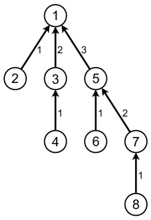
Figure 1: Binomial tree structure defining the parallel model.

In more detail, we have seen in Section 3.3 that it is possible for the leader to obtain ($k+2$)-bit approximations of $\mathrm{a}_{1}(B)=\prod_{j=1}^{n}c_{j}$ and $\mathrm{a}_{2}(B)=\prod_{j=1}^{n}s_{j}$ at an expected communication cost of $O(kn+n\log n)$ bits. To bring this down to $O(k\log n+\log^{2}\!n)$ time, we let the parties communicate with one another according to the binomial tree structure shown in Fig. 1, in which numbers in the nodes correspond to parties (the leader is number 1 at the root) and numbers next to the arrows correspond to the order in which data is transmitted. For simplicity, we may assume that $n$ is a power of $2$. To understand the algorithm, think of a tree with nodes containing $s_{j}$ and $c_{j}$, for $1\leq j\leq n$. Node number $j$ can be thought of as belonging to party number $j$, who knows $s_{j}$ and $c_{j}$ exactly. We pair parties by groups of $2$. For a given pair, say $(j,j+1)$, with $j$ odd, party $j+1$ sends $\hat{s}_{j+1}$ and $\hat{c}_{j+1}$ to party $j$, who computes $\hat{s}_{j}\hat{s}_{j+1}$ and $\hat{c}_{j}\hat{c}_{j+1}$. Then, party $j$ is matched with party $j+2$, where $j-1$ is divisible by 4. This process gives rise to the new pair $(j,j+2)$, from which emerges the products $\hat{s}_{j}\hat{s}_{j+1}\hat{s}_{j+2}\hat{s}_{j+3}$ and $\hat{c}_{j}\hat{c}_{j+1}\hat{c}_{j+2}\hat{c}_{j+3}$, and so on up to the leader, who is party 1 at the root of the tree.

Algorithm 5 Computing products in parallel, communicating along a binomial tree configuration

1:  If $n$ is not a power of $2$, add virtual parties with $c_{j}=s_{j}=1$ for $n<j\leq 2^{\lceil\,\log_{2}n\rceil}${These parties, being dummy, have no effect on the overall communication complexity}

2:  $\ell\leftarrow k+3+\lceil\,\log_{2}n\rceil$

3:  for $j\leftarrow 1$ to $n$ in parallel do

4:     Party $j$ does $\tilde{c}_{j}\leftarrow\hat{c}_{j}$ and $\tilde{s}_{j}\leftarrow\hat{s}_{j}$, which are $\ell$-bit truncations of $c_{j}$ and $s_{j}$, respectively.

5:  end for

6:  $m\leftarrow 1$

7:  repeat

8:     for $j\leftarrow 1$ to $n$ by step of $2m$ in parallel do

9:        Party $j+m$ sends $\tilde{c}_{j+m}$ and $\tilde{s}_{j+m}$ to party $j$

10:        Party $j$ computes $\tilde{c}_{j}\leftarrow\tilde{c}_{j}\,\tilde{c}_{j+m}$ and $\tilde{s}_{j}\leftarrow\tilde{s}_{j}\,\tilde{s}_{j+m}$, both truncated to $\ell$ bits

11:     end for

12:     $m\leftarrow 2m$

13:  until $m\geq n$

14:  Party 1 (the leader) outputs $\tilde{c}_{1}$ and $\tilde{s}_{1}$

This approach is formalized in Algorithm 5, in which new variables $\tilde{c}_{j}$ and $\tilde{s}_{j}$ are introduced to hold approximations of products of increasingly many $c$’s and $s$’s as the process unfolds. The issue of the required precision at each level of the process has to be reconsidered because the leader will no longer receive the entire list of $\hat{c}_{j}$’s and $\hat{s}_{j}$’s since subproducts are calculated en route by intermediate parties, which must be truncated for transmission. For simplicity, we proceed as if all the $c_{j}$’s and $s_{j}$’s were nonnegative and we percolate the signs up the tree separately. We know from Theorem 1, using $v=0$, that if $\hat{x}$ and $\hat{y}$ are $\ell$-bit approximations (in particular $\ell$-bit truncations) of $x$ and $y$, respectively, for arbitrary real numbers $x$ and $y$ in $[0,1]$ and integer $\ell$, then $\hat{x}\hat{y}$ is an ($\ell-1$)-bit approximation of $xy$. However, $\hat{x}\hat{y}$ is not in general an ($\ell-1$)-bit truncation of $xy$ because it could have up to $2\ell$ bits of precision and we do not want to transmit so many bits up the binomial tree. There is an apparent problem if we transmit the $\ell$-bit truncation of $\hat{x}\hat{y}$ instead, as we do indeed in Algorithm 5, because it is an ($\ell-2$)-bit approximation of $xy$, but not necessarily an ($\ell-1$)-bit approximation. Nevertheless, it is shown in Appendix B that the recursive application of pairwise multiplications followed by truncation to $\ell$ bits results in the loss of only one bit of precision per subsequent level. Thus, on the $i^{\mathrm{th}}$ time round the repeat loop, $1\leq i\leq\lceil\,\log_{2}n\rceil$, the numbers calculated at line 10, even after truncation to $\ell$ bits, are ($\ell-i-1$)-bit approximations of the exact product that they represent (again, up to sign, which is handled separately). It follows that the final numbers computed by the leader when $i=\lceil\,\log_{2}n\rceil$ are ($k+2$)-bit approximations of the products of all the $c_{j}$’s and the $s_{j}$’s, as required, provided we start with $\ell=k+3+\lceil\,\log_{2}n\rceil$.

To analyse the communication complexity of this strategy, we consider that bits sent and received in parallel between disjoint pairs of parties count as a single time step in the global communication process. The repeat loop is carried out $\lceil\,\log_{2}n\rceil$ times. Each time round this loop, parties transmit in parallel two $\ell$-bit approximations, which require $\ell+1$ bits of communication per active party since signs must also be transmitted. It follows immediately that the parallel complexity of Algorithm 5 is $2(\ell+1)\lceil\,\log_{2}n\rceil=2(k+4+\lceil\,\log_{2}n\rceil)\lceil\,\log_{2}n\rceil$, which is $O(k\log n+\log^{2}\!n$). Therefore, this takes $O(k\log n)$ time provided $k>\log_{2}n$.

Now, let us use Algorithm 5 to replace lines 17 and 18 in Algorithm 4. This allows the leader to obtain his required $(k+2)$-bit approximations of $\mathrm{a}_{1}(B)$ and $\mathrm{a}_{2}(B)$ with no need for him to learn all the $(k+2+\lceil\,\log_{2}n\rceil)$-bit truncations of $c_{j}$ and $s_{j}$ from each party $j\geq 2$. We have just seen that $O(k\log n+\log^{2}\!n$) parallel time suffices for this task. Unfortunately, this improvement is incompatible with the idea of transmitting only one more bit of information for each $c_{j}$ and $s_{j}$ when $k$ is increased by $1$, which was crucial in the efficiency of the sequential version of Algorithm 4 studied in Section 4. The problem stems from the fact that the $\ell$-bit truncation of the product of the $\ell$-bit truncations of $x$ and $y$ can be entirely different from the $(\ell+1)$-bit truncation of the product of the $(\ell+1)$-bit truncations of the same numbers. This is illustrated with $x=0.1111\ldots$ and $y=0.1001\ldots$ (in binary, of course). If we take $\ell=3$, the truncations of $x$ and $y$ are $0.111$ and $0.100$, respectively, whose product is $0.011100$. In contrast, with $\ell=4$, the truncations of $x$ and $y$ are $0.1111$ and $0.1001$, respectively, whose product is $0.10000111$. We see that the $3$-bit truncation of the product of the $3$-bit truncations is $0.011$, whereas the $4$-bit truncation of the product of the $4$-bit truncations is $0.1000$, which are different on each and every bit of the fractional part! This demonstrates the fact that the bits going up the binomial tree in Algorithm 5 can change drastically from one run to the next even if a single bit of precision is added to all nodes at the bottom level, and therefore that we have to start afresh for each new value of $k$. As a consequence, the use of Algorithm 5 to replace lines 17 and 18 in Algorithm 4 results in an “improvement” in which we expect to have to transmit $\Omega(n^{3})$ bits, taking $\Omega(n^{2}\log n)$ parallel time to do so!

Fortunately, there is an easy cure to this problem, which we only sketch here. In addition to using Algorithm 5 to replace lines 17 and 18 in Algorithm 4, we also change line 25 from “$k\leftarrow k+1$” to “$k\leftarrow 2k$”. Even though parties have to transmit up the binomial tree the entire $(k+3+\lceil\,\log_{2}n\rceil)$-bit truncations of each $c_{j}$ and $s_{j}$ for each new value of $k$, the work done each time round the loop is roughly equivalent to the sum of all the work done until then. Since we expect to succeed when $k$ is roughly equal to $n$, the expected total parallel time is about twice $O(k\log n+\log^{2}\!n$) with $k\approx n$, which is simply $O(n\log n)$. The expected total number of bits communicated with this approach is slightly greater than with Algorithm 4, but remains $O(n^{2})$.

5.2 Reducing the number of rounds

Algorithm 4 is efficient in terms of the number of bits of randomness as well as the number of bits of communication, but it requires an expected $O(n)$ rounds, in which the leader and all other parties take turn at sending messages. This could be prohibitive if they are far apart and their purpose is to try to convince examiners that they are actually using true entanglement and quantum processes to produce their joint outputs, because it would prevent them from responding quickly enough to be credible. The solution should be rather obvious at this point, and we leave the details to the reader. If we change line 25 from “$k\leftarrow k+1$” to “$k\leftarrow 2k$”, the expected number of rounds is decreased from $O(n)$ to $O(\log n)$. If in addition we start with “$k\leftarrow n$” instead of “$k\leftarrow 1$” at line 12, the expected number of rounds becomes a constant. (Alternatively, we could start with “$k\leftarrow n$” at line 12 and step with “$k\leftarrow k+n$” at line 25.)

5.3 Equatorial measurements

Recall that equatorial measurements are those for which $\varphi_{j}=0$ for each party $j$. In this case, the leader can sample according to $p_{1}$ or $p_{2}$, without any help or communication from the other parties, since he has complete knowledge of their vanished elevation angles. Therefore, he can run lines 5 to 28 of Algorithm 4 all by himself! However, he still needs to communicate in line 1 of Algorithm 4 in order to know from which of $p_{1}$ or $p_{2}$ to sample. The only remaining need for communication occurs in line 29, which has to be modified from “The leader informs all the other parties that the simulation is complete” to “The leader informs all the other parties of which value of $B_{j}\in\{-1,+1\}$ he has chosen for them”.

Only line 1 requires significant communication since the new line 29 needs only the transmission of $n-1$ bits. We have already seen at the end of Section 3.2 that line 1, which is a distributed version of Algorithm 1, requires an expected communication of $O(n\log n)$ bits in the sequential model. This is therefore the complexity of our simulation, which is an improvement over the previously best technique known to simulate the GHZ distribution under arbitrary equatorial von Neumann measurements [7], which required an expectation of $O(n^{2})$ bits of communication.

A more elegant protocol can be obtained if we use Equation (16) at the end of Appendix A, which gives us a simplified formula for $p(b)$ in the case of equatorial measurements. Each party $j$ other than the leader can simply choose an independent unbiased Rademacher $b_{j}\in\{-1,+1\}$ as final output, without any consideration of his own input $\theta_{j}$ nor communication with anyone else, and inform the leader of this choice. It simply remains for the leader to choose his own $b_{1}$ in order to make $\prod_{j=1}^{n}b_{j}$ equal to $+1$ with probability $\cos^{2}(\theta/2)$ or $-1$ with complementary probability $\sin^{2}(\theta/2)$. For this, we still need line 1 from Algorithm 4, which requires an expected communication of $O(n\log n)$ bits.

To adapt this latter protocol to the parallel model, note that the leader does not need to know all the $b_{j}$’s chosen by the other parties since he only needs their product, which is either $+1$ or $-1$. It is elementary to adapt Algorithm 5 in order to percolate this information to the leader up the binomial tree, at a communication cost of $O(n)$ bits but only $O(\log n)$ parallel time. One can also adapt Algorithm 5 to work with sums instead of products, which is the relevant operation to parallelize the distributed version of Algorithm 1. Sums and products are similar since if $\hat{x}$ and $\hat{y}$ are $t$-bit approximations of $x$ and $y$, respectively, for an arbitrary integer $t$, then $\hat{x}+\hat{y}$ and $\hat{x}\hat{y}$ are $(t-1)$-bit approximations of $x+y$ and $xy$, respectively, according to Theorem 1, using $v=0$. However, parallelizing sums is easier than products because the exact sum $\hat{x}+\hat{y}$ can be transmitted with no more bits of precision than each of $\hat{x}$ and $\hat{y}$, even though one additional bit is required to transmit the integer part of the sum,  whereas the product $\hat{x}\hat{y}$ could entail twice as many bits of precision than each of $\hat{x}$ and $\hat{y}$ (this is why we needed Appendix B). In round $k$ of the loop in Algorithm 1, the leader needs to obtain a $k$-bit approximation of $\cos^{2}(\sum_{j=1}^{n}\theta_{j}/2)$, which in turn requires the addition of $\ell=k+3+\lceil\,\log_{2}n\rceil$ bits from each of the $n-1$ half-angles $\theta_{j}/2$ owned by the various parties $j\geq 2$. The binomial tree construction makes it possible to percolate this sum up to the leader through $\lceil\,\log_{2}n\rceil$ levels in which it is sufficient to transmit $\ell+i$ bits up the tree for each partial sum (or initial half angle) at distance $i$ from the leaves. The expected cost before the leader obtains the required $k$-bit approximation of $\cos^{2}(\sum_{j=1}^{n}\theta_{j}/2)$ is therefore $O((k+\log n)\,n)$ bits of communications but only $O((k+\log n)\log n)$ parallel time. Using once again the fact that the expected number $k$ of rounds in Algorithm 1 is bounded by $5$, the required Bernoulli variable with parameter $\cos^{2}(\sum_{j=1}^{n}\theta_{j}/2)$ can be sampled exactly after an expected communication cost of $O(n\log n)$ bits, as in the sequential model, but only $O(\log^{2}\!n)$ parallel time. This dominates the cost of the parallel implementation of our algorithm in the case of equatorial measurements.

Note that all this information is sent up the binomial tree towards the leader. The only information that the leader has to send back down to the other parties, each time round the loop, serves to notify them of whether or not a more precise approximation of their azimuthal angles is required in order to complete the Bernoulli sampling. This bit can be sent down the binomial tree at the cost of $O(\log n)$ time if we reverse the arrows in Figure 1 and reorder the transmissions from the edge marked $\lceil\,\log_{2}n\rceil$ (which is $\lceil\,\log_{2}8\rceil=3$ in the figure) down to the edges marked $1$.

If we consider a nonstandard model in which we only care about what happens until all parties have produced their output, we can modify the above protocol to require only one-way communication on each of the links, namely up the binomial tree, with no increase (in fact a small decrease) in expected communication and time complexities before the final output has been produced. For this, we simply remove the leader’s notification to all other parties of whether or not the simulation has been completed. This means that all parties will indefinitely continue to provide the leader (who will pay no attention!) with increasingly precise approximations of the sum of their azimuthal angles, but this useless activity will take place after all parties have produced their output. Indeed, all parties other than the leader can output their randomly selected $+1$ or $-1$ at the very beginning of the protocol, and the leader can output his answer as soon as he knows that the Bernoulli sampling (Algorithm 1) has been successful.

Of course, we could have parallelized line 1 of Algorithm 4 even in the case of non-equatorial measurements. However, this would not have impacted significantly on the overall time complexity of our general solution, which remains $O(n\log n)$.

5.4 Only the leader needs to be probabilistic

It is easy to modify almost all our protocols to require randomness only from the leader, all other parties being purely deterministic. For this, notice that the total expected amount of randomness is only $O(n)$, which is negligible compared to the total number of bits that have to be communicated. Hence, each time one party needs a random bit, he can ask the leader to provide it. This will only increase the communication cost by an expected $O(n)$ bits, which has no effect on the overall asymptotic communication complexity of our protocols. The same remark applies to the time required by our protocols in the parallel model, with the exception of the case of equatorial measurements, in which an $O(\log^{2}\!n)$ expected time requires all parties other than the leader to choose their unbiased random output in parallel.

6 Conclusion, discussion and open problems

We have addressed the problem of simulating the effect of arbitrary independent von Neumann measurements on the qubits forming the general GHZ state $\raisebox{0.17218pt}[0.0pt][0.0pt]{\small$\textstyle\frac{1}{\sqrt{2}}$}|0^{n}\rangle+\raisebox{0.17218pt}[0.0pt][0.0pt]{\small$\textstyle\frac{1}{\sqrt{2}}$}|1^{n}\rangle$ distributed among $n$ parties. Rather than doing the actual quantum measurements, the parties must sample the exact GHZ probability distribution by purely classical means, which necessarily requires communication in view of Bell’s theorem. Our main objective was to find a protocol that solves this conundrum with a finite amount of expected communication, which had only been known previously to be possible when the von Neumann measurements are restricted to being equatorial (a severe limitation indeed). Our solution needs only an expectation of $O(n^{2})$ bits of communication, which can be dispatched in $O(n\log n)$ expected time if bits can be sent in parallel according to a realistic scenario in which nobody has to send or receive more than one bit in any given step. We also improved on the former art in the case of equatorial measurements, with expectations of $O(n\log n)$ bits of communication and $O(\log^{2}\!n)$ parallel time.

Knuth and Yao [18] initiated the study of the complexity of generating random integers (or bit strings) with a given probability distribution $p$, assuming only the availability of a source of unbiased identically independently distributed random bits. They showed that any sampling algorithm must use an expected number of bits at least equal to the entropy $\sum_{b}p(b)\log_{2}(1/p(b))$ of the distribution, and that the best algorithm does not need more than two additional bits. For further results on the bit model in random variate generation, see Ref. [10, Chap. XIV] and Ref. [11].

The GHZ distribution has an entropy no larger than $n$, and therefore Knuth and Yao have shown that it could be sampled with no more than $n+2$ expected random bits if all the parameters were concentrated in a single place. Even though we have studied the problem of sampling this distribution in a setting in which the defining parameters (here the description of the von Neumann measurements) are distributed among $n$ parties, and despite the fact that our main purpose was to minimize communication between these parties, we were able to succeed with $6n+17$ expected random bits, which is just above six times the bound of Knuth and Yao. The amount of randomness required by our protocols does not depend significantly on the actual measurements they have to simulate, as discussed at the end of Section 4.2. However, some sets of measurements entail a probability distribution $p$ whose entropy $H(p)$ is much smaller than $n$. In the extreme case of having all measurements in the computational basis, $H(p)$ is a single bit! Can there be protocols that succeed with as few as $H(p)+2$ expected random bits, thus meeting the bound of Knuth and Yao, or failing this as few as $O(H(p))$ expected random bits, no matter how small $H(p)$ is for the given set of von Neumann measurements? Notice that all the protocols presented here require $\Omega(n)$ random bits since they ask each party to sample independently at least once a Rademacher random variable, a hurdle that can only be alleviated in the case of measurements in the computational basis. It may be that this problem can be solved if we put the leader in charge of drawing all the Rademachers in a single batch. But what would be the cost in terms of communication from the other parties, who will need to send sufficiently precise approximations of their elevation angles $\varphi_{j}$ to the leader, rather than the much easier task of generating their own Rademachers locally?

Are our protocols optimal in terms of the required amount of communication? Could we simulate arbitrary von Neumann measurements as efficiently as in the case of equatorial measurements, i.e. with $O(n\log n)$ expected bits of communication? We leave this as open question, but point out that Broadbent, Chouha and Tapp have proved an $\Omega(n\log n)$ lower bound on the worst case communication complexity of simulating measurements on $n$-partite GHZ states [8], a result that holds even for equatorial measurements, and even under the promise that $\cos\sum_{j=1}^{n}\theta_{j}=\pm 1$ [17].

As a recent development, which will be the subject of a follow-up paper [6], we have discovered how to handle arbitrary $n$-partite states, such as the tripartite $W$ state $\raisebox{0.17218pt}[0.0pt][0.0pt]{\small$\textstyle\frac{1}{\sqrt{3}}$}|100\rangle+\raisebox{0.17218pt}[0.0pt][0.0pt]{\small$\textstyle\frac{1}{\sqrt{3}}$}|010\rangle+\raisebox{0.17218pt}[0.0pt][0.0pt]{\small$\textstyle\frac{1}{\sqrt{3}}$}|001\rangle$ and its $n$-partite generalization

$$W_{n}={\textstyle\frac{1}{\sqrt{n}}}\,\big{(}|10^{n-1}\rangle+|010^{n-2}\rangle+|0010^{n-3}\rangle+\cdots+|0^{n-1}1\rangle\big{)}\,,$$

in which each of the $n$ parties is given one of the qubits. Although the general simulation process is rather more complicated and slightly less efficient than in the case of the GHZ state, the effect of $n$ independent von Neumann measurements on any $n$-partite state (even a mixed state) distributed among $n$ participants can be simulated with an expectation of $(5+o(1))n^{2}$ bits of communication. Only the leader needs access to a source of randomness and an expectation of $(4+o(1))n^{2}$ unbiased identically independently distributed bits suffices to carry out the simulation.

We leave for further research the problem of simulating arbitrary positive-operator-valued measurements (POVMs) on the single-qubit shares of GHZ states (or on more general multipartite states), as well as the problem of simulating multipartite entanglement (other than the already-solved equatorial von Neumann measurements on the tripartite GHZ state [3]) with worst-case bounded classical communication.

Appendices

Appendix A Convex decomposition of the GHZ distribution

Our simulation of the GHZ distribution hinges upon its decomposition into a convex combination of two sub-distributions, which is stated as Equation (1) at the beginning of Section 2,

$$\textstyle p(b)=\cos^{2}\!\big{(}\frac{\theta}{2}\big{)}\,p_{1}(b)+\sin^{2}\!\big{(}\frac{\theta}{2}\big{)}\,p_{2}(b)\,,$$

in which the coefficients $\cos^{2}(\theta/2)$ and $\sin^{2}(\theta/2)$ depend only on the equatorial part of the measurements, whereas the sub-distributions depend only on their real part. This decomposition was obtained by one of us [14, 15], albeit in the usual computer science language in which von Neumann measurements are presented as a unitary transformation followed by a measurement in the computational basis. For completeness, here we derive this decomposition directly in the language of von Neumann measurements.

First, let us recall some facts, including some already mentioned in Section 2. We begin with a $2\times 2$ von Neumann measurement, which can be written as

$$M=x\sigma_{1}+y\sigma_{2}+z\sigma_{3}=x\left(\begin{array}[]{cc}0&1\\ 1&0\\ \end{array}\right)+y\left(\begin{array}[]{cc}0&-\imath\\ \imath&0\\ \end{array}\right)+z\left(\begin{array}[]{cc}1&0\\ 0&-1\\ \end{array}\right)=\left(\begin{array}[]{cc}z&x-\imath y\\ x+\imath y&-z\\ \end{array}\right)\,,$$

where $x^{2}+y^{2}+z^{2}=1$. Thus, using spherical coordinates $(\theta,\varphi)\in[0,2\pi)\times[-\pi/2,\pi/2]$, the parameters $(x,y,z)$ can be written as

$$x = \cos\theta\cos\varphi$$

$$y = \sin\theta\cos\varphi$$

$$z = \sin\varphi$$

so that

$$M=\left(\begin{array}[]{cc}\sin\varphi&e^{-\imath\theta}\cos\varphi\\ e^{\imath\theta}\cos\varphi&-\sin\varphi\end{array}\right)\,.$$

The spectra (set of eigenvalues) of $M$ is $\{-1,+1\}$ and the unitary operator $U$ that diagonalizes $M$ is given by

$$U=\left(\begin{array}[]{cc}\alpha&-\bar{\beta}\\ -\beta&-\bar{\alpha}\end{array}\right)$$

with

$$\alpha=\cos\Big{(}\frac{\varphi}{2}-\frac{\pi}{4}\Big{)}~{}~{}\text{and}~{}~{}\beta=e^{\imath\theta}\sin\Big{(}\frac{\varphi}{2}-\frac{\pi}{4}\Big{)}\,.$$

In other words, we have

$$M=U\left(\begin{array}[]{cc}1&0\\ 0&-1\end{array}\right)U^{\dagger}.$$

The density matrix representing the GHZ state can be decomposed as

$$\rho=|\Psi_{n}\rangle\langle\Psi_{n}|=\frac{1}{2}\left(\bigotimes_{j=1}^{n}{\left(\begin{array}[]{cc}1&0\\ 0&0\end{array}\right)}+\bigotimes_{j=1}^{n}{\left(\begin{array}[]{cc}0&1\\ 0&0\end{array}\right)}+\bigotimes_{j=1}^{n}{\left(\begin{array}[]{cc}0&0\\ 1&0\end{array}\right)}+\bigotimes_{j=1}^{n}{\left(\begin{array}[]{cc}0&0\\ 0&1\end{array}\right)}\right)\,.$$

Before analysing the joint probability function, we point out that

$$|b\rangle\langle b|=\left(\begin{array}[]{cc}\delta_{+1}(b)&0\\ 0&\delta_{-1}(b)\end{array}\right),$$

where $b\in\{-1,+1\}$, $|+1\rangle={\,1\,\choose\,0\,}$, $|-1\rangle={{\,0\,}\choose{\,1\,}}$ and $\delta$ is the Kronecker delta function $\delta_{x}(y)=1$ if $x=y$ and $\delta_{x}(y)=0$ if $x\neq y$. We also invite the reader to verify that

$$\mathrm{Tr}\Bigg{(}\bigg{(}|b\rangle\langle b|\bigg{)}U\left(\begin{array}[]{cc}1&0\\ 0&0\end{array}\right)U^{\dagger}\Bigg{)} = |\alpha|^{2}\delta_{+1}(b)+|\beta|^{2}\delta_{-1}(b)$$

$$= \cos^{2}\!\bigg{(}\frac{1}{2}\Big{(}\varphi-\frac{\pi}{2}b\Big{)}\bigg{)}$$

$$\mathrm{Tr}\Bigg{(}\bigg{(}|b\rangle\langle b|\bigg{)}U\left(\begin{array}[]{cc}0&1\\ 0&0\end{array}\right)U^{\dagger}\Bigg{)} = -\alpha\beta\delta_{+1}(b)+\alpha\beta\delta_{-1}(b)$$

$$= -e^{\imath\theta}\sin\!\bigg{(}\frac{1}{2}\Big{(}\varphi-\frac{\pi}{2}b\Big{)}\bigg{)}\cos\!\bigg{(}\frac{1}{2}\Big{(}\varphi-\frac{\pi}{2}b\Big{)}\bigg{)}$$

$$\mathrm{Tr}\Bigg{(}\bigg{(}|b\rangle\langle b|\bigg{)}U\left(\begin{array}[]{cc}0&0\\ 1&0\end{array}\right)U^{\dagger}\Bigg{)} = -\bar{\alpha}\bar{\beta}\delta_{+1}(b)+\bar{\alpha}\bar{\beta}\delta_{-1}(b)$$

$$= -e^{-\imath\theta}\sin\!\bigg{(}\frac{1}{2}\Big{(}\varphi-\frac{\pi}{2}b\Big{)}\bigg{)}\cos\!\bigg{(}\frac{1}{2}\Big{(}\varphi-\frac{\pi}{2}b\Big{)}\bigg{)}$$

$$\mathrm{Tr}\Bigg{(}\bigg{(}|b\rangle\langle b|\bigg{)}U\left(\begin{array}[]{cc}0&0\\ 0&1\end{array}\right)U^{\dagger}\Bigg{)} = |\beta|^{2}\delta_{+1}(b)+|\alpha|^{2}\delta_{-1}(b)$$

$$= \sin^{2}\!\bigg{(}\frac{1}{2}\Big{(}\varphi-\frac{\pi}{2}b\Big{)}\bigg{)}\,.$$

For convenience, let

$$E_{1}=\left(\begin{array}[]{cc}1&0\\ 0&0\end{array}\right),~{}E_{2}=\left(\begin{array}[]{cc}0&1\\ 0&0\end{array}\right),~{}E_{3}=\left(\begin{array}[]{cc}0&0\\ 1&0\end{array}\right)~{}\text{and}~{}E_{4}=\left(\begin{array}[]{cc}0&0\\ 0&1\end{array}\right).$$

Given $n$ von Neumann measurements $M_{j}$, $1\leq j\leq n$, the joint probability $p(b)$ of obtaining $b\in\{-1,+1\}^{n}$ as a result of applying these measurements on an $n$-partite GHZ state is

$$p(b) = |\langle b|U|\Psi_{n}\rangle|^{2}$$

$$= \mathrm{Tr}\Big{(}\langle b|U|\Psi_{n}\rangle\big{(}\langle b|U|\Psi_{n}\rangle\big{)}^{\dagger}\Big{)}$$

$$= \mathrm{Tr}\Big{(}\langle b|U|\Psi_{n}\rangle\langle\Psi_{n}|U^{\dagger}|b\rangle\Big{)}$$

$$= \mathrm{Tr}\bigg{(}\Big{(}|b\rangle\langle b|\Big{)}U\rho{}\,U^{\dagger}\bigg{)}$$

$$= \frac{1}{2}\mathrm{Tr}\Bigg{(}\bigotimes_{j=1}^{n}{|b_{j}\rangle\langle b_{j}|}\Bigg{(}\bigotimes_{j=1}^{n}{U_{j}E_{1}U_{j}^{\dagger}}+\bigotimes_{j=1}^{n}{U_{j}E_{2}U_{j}^{\dagger}}+\bigotimes_{j=1}^{n}{U_{j}E_{3}U_{j}^{\dagger}}+\bigotimes_{j=1}^{n}{U_{j}E_{4}U_{j}^{\dagger}}\Bigg{)}\Bigg{)}$$

$$= \frac{1}{2}\sum_{i=1}^{4}{\prod_{j=1}^{n}{\mathrm{Tr}\Bigg{(}\left(\begin{array}[]{cc}\delta_{+1}(b_{j})&0\\ 0&\delta_{-1}(b_{j})\end{array}\right)U_{j}E_{i}U_{j}^{\dagger}\Bigg{)}}}\,.$$

Putting these equations together, we have:

$$\prod_{j=1}^{n}{\mathrm{Tr}\Bigg{(}\left(\begin{array}[]{cc}\delta_{+1}(b_{j})&0\\ 0&\delta_{-1}(b_{j})\end{array}\right)U_{j}E_{1}U_{j}^{\dagger}\Bigg{)}} = \prod_{j=1}^{n}{\cos^{2}\!\bigg{(}\frac{1}{2}\Big{(}\varphi_{j}-\frac{\pi}{2}b_{j}\Big{)}\bigg{)}}~{}~{}\stackrel{{\scriptstyle\textrm{def}}}{{=}}~{}~{}f_{1}$$

$$\prod_{j=1}^{n}{\mathrm{Tr}\Bigg{(}\left(\begin{array}[]{cc}\delta_{+1}(b_{j})&0\\ 0&\delta_{-1}(b_{j})\end{array}\right)U_{j}E_{2}U_{j}^{\dagger}\Bigg{)}} = \prod_{j=1}^{n}{-e^{\imath\theta_{j}}\sin\!\bigg{(}\frac{1}{2}\Big{(}\varphi_{j}-\frac{\pi}{2}b_{j}\Big{)}\bigg{)}\cos\!\bigg{(}\frac{1}{2}\Big{(}\varphi_{j}-\frac{\pi}{2}b_{j}\Big{)}\bigg{)}}~{}~{}\stackrel{{\scriptstyle\textrm{def}}}{{=}}~{}~{}f_{2}$$

$$\prod_{j=1}^{n}{\mathrm{Tr}\Bigg{(}\left(\begin{array}[]{cc}\delta_{+1}(b_{j})&0\\ 0&\delta_{-1}(b_{j})\end{array}\right)U_{j}E_{3}U_{j}^{\dagger}\Bigg{)}} = \prod_{j=1}^{n}{-e^{-\imath\theta_{j}}\sin\!\bigg{(}\frac{1}{2}\Big{(}\varphi_{j}-\frac{\pi}{2}b_{j}\Big{)}\bigg{)}\cos\!\bigg{(}\frac{1}{2}\Big{(}\varphi_{j}-\frac{\pi}{2}b_{j}\Big{)}\bigg{)}}~{}~{}\stackrel{{\scriptstyle\textrm{def}}}{{=}}~{}~{}f_{3}$$

$$\prod_{j=1}^{n}{\mathrm{Tr}\Bigg{(}\left(\begin{array}[]{cc}\delta_{+1}(b_{j})&0\\ 0&\delta_{-1}(b_{j})\end{array}\right)U_{j}E_{4}U_{j}^{\dagger}\Bigg{)}} = \prod_{j=1}^{n}{\sin^{2}\!\bigg{(}\frac{1}{2}\Big{(}\varphi_{j}-\frac{\pi}{2}b_{j}\Big{)}\bigg{)}}~{}~{}\stackrel{{\scriptstyle\textrm{def}}}{{=}}~{}~{}f_{4}\,.$$

Thus, $p(b)=\frac{1}{2}(f_{1}+f_{2}+f_{3}+f_{4})$.

Keeping in mind that

$$f_{2}+f_{3}=2\cos\!\bigg{(}\sum_{j=1}^{n}{\theta_{j}}\bigg{)}\prod_{j=1}^{n}{-\sin\!\bigg{(}\frac{1}{2}\Big{(}\varphi_{j}-\frac{\pi}{2}b_{j}\Big{)}\bigg{)}\cos\!\bigg{(}\frac{1}{2}\Big{(}\varphi_{j}-\frac{\pi}{2}b_{j}\Big{)}\bigg{)}}$$

and

$$x^{2}+y^{2}+2xy\cos\gamma=(x+y)^{2}\cos^{2}(\gamma/2)+(x-y)^{2}\sin^{2}(\gamma/2)$$

for all real numbers $x$ and $y$, and angle $\gamma$, it follows that

$$p(b) = \cos^{2}\!\Bigg{(}\frac{1}{2}\sum_{j=1}^{n}{\theta_{j}}\Bigg{)}\Bigg{(}\frac{\prod_{j=1}^{n}{\cos\big{(}\frac{1}{2}\big{(}\varphi_{j}-\frac{\pi}{2}b_{j}\big{)}\big{)}}+\prod_{j=1}^{n}{-\sin\big{(}\frac{1}{2}\big{(}\varphi_{j}-\frac{\pi}{2}b_{j}\big{)}\big{)}}}{\sqrt{2}}\Bigg{)}^{\!\!2}\,+$$

$$\sin^{2}\!\Bigg{(}\frac{1}{2}\sum_{j=1}^{n}{\theta_{j}}\Bigg{)}\Bigg{(}\frac{\prod_{j=1}^{n}{\cos\big{(}\frac{1}{2}\big{(}\varphi_{j}-\frac{\pi}{2}b_{j}\big{)}\big{)}}-\prod_{j=1}^{n}{-\sin\big{(}\frac{1}{2}\big{(}\varphi_{j}-\frac{\pi}{2}b_{j}\big{)}\big{)}}}{\sqrt{2}}\Bigg{)}^{\!\!2}\,.$$

If we define

$$\mathrm{a}_{1}(b) =\prod_{j=1}^{n}\textstyle{\cos\big{(}\frac{1}{2}\big{(}\varphi_{j}-\frac{\pi}{2}b_{j}\big{)}\big{)}}, \mathrm{a}_{2}(b) =\prod_{j=1}^{n}\textstyle{-\sin\big{(}\frac{1}{2}\big{(}\varphi_{j}-\frac{\pi}{2}b_{j}\big{)}\big{)}}\,,$$

$$p_{1}(b) =\frac{1}{2}\big{(}\mathrm{a}_{1}(b)+\mathrm{a}_{2}(b)\big{)}^{2}, p_{2}(b) =\frac{1}{2}\big{(}\mathrm{a}_{1}(b)-\mathrm{a}_{2}(b)\big{)}^{2}\,,$$

this is precisely the convex decomposition

$$\textstyle p(b)=\cos^{2}\!\big{(}\frac{\theta}{2}\big{)}\,p_{1}(b)+\sin^{2}\!\big{(}\frac{\theta}{2}\big{)}\,p_{2}(b)\,,$$

where $\theta=\sum_{j=1}^{n}\theta_{j}$, that was given as Equation (1) at the beginning of Section 2.

As a “reality check”, we analyse this formula for the special case of equatorial measurements, in which all elevation angles vanish. The formulas for $a_{1}(b)$ and $a_{2}(b)$, and therefore those for $p_{1}(b)$ and $p_{2}(b)$, become very simple when $\varphi_{j}=0$ for all $j$. For any $b=(b_{1},\ldots,b_{n})\in\{-1,+1\}^{n}$, let us define $s(b)=\prod_{j=1}^{n}b_{j}\in\{-1,+1\}$ and $X=\{b\in\{-1,+1\}^{n}\mid s(b)=+1\}$. It is easy to see that $a_{1}(b)=2^{-n/2}$ and $a_{2}(n)=(-1)^{s(b)}2^{-n/2}$. Therefore,

$$p_{1}(b)=\left\{\begin{array}[]{ll}2^{1-n}&\mbox{if~{}}b\in X\\ 0&\mbox{if~{}}b\not\in X\end{array}\right.\mbox{~{}~{}~{}and~{}~{}~{}}p_{2}(b)=\left\{\begin{array}[]{ll}0&\mbox{if~{}}b\in X\\ 2^{1-n}&\mbox{if~{}}b\not\in X\,.\end{array}\right.$$

Hence,

$$p(b)=\left\{\begin{array}[]{ll}2^{1-n}\cos^{2}\!\big{(}\frac{\theta}{2}\big{)}&\mbox{if~{}}b\in X\\[6.45831pt] 2^{1-n}\sin^{2}\!\big{(}\frac{\theta}{2}\big{)}&\mbox{if~{}}b\not\in X\,.\end{array}\right.$$ (16)

Thus, in the case of equatorial measurements, we obtain a uniformly distributed $b\in X$ with probability $\cos^{2}(\theta/2)$ or a uniformly distributed $b\in\{-1,+1\}^{n}\setminus X$ with complementary probability $\sin^{2}(\theta/2)$. From this, it follows immediately that the expected value of the product of the $b_{j}$’s is equal to the cosine of the sum of the azimuthal angles because

$$\mathbf{E}\Big{\{}\prod_{j=1}^{n}b_{j}\Big{\}}=\textstyle\cos^{2}\!\big{(}\frac{\theta}{2}\big{)}\times(+1)+\sin^{2}\!\big{(}\frac{\theta}{2}\big{)}\times(-1)=\cos^{2}\!\big{(}\frac{\theta}{2}\big{)}-\sin^{2}\!\big{(}\frac{\theta}{2}\big{)}=\cos\theta=\displaystyle\cos\!\Big{(}\sum_{j=1}^{n}\theta_{j}\Big{)}\,.$$

It follows equally easily that $\mathbf{E}\big{\{}\prod_{j\in J}b_{j}\big{\}}=0$ for any nonempty $J\subsetneq\{1,\ldots,n\}$, and therefore all the marginal probability distributions obtained by tracing out one or more of the parties are uniform. Those well-known facts were indeed the formulas used in the prior art of simulating equatorial measurements on GHZ states [1, 3, 7].

Appendix B Approximations and truncations of products

In this appendix, we restrict our attention to the multiplication of real numbers in the interval $[0,1]$ because this is what is relevant to the analysis of the parallel model, in which we need to approximate the product of sines and cosines sent up the binomial tree of Figure 1. It is sufficient, again for simplicity, to concentrate on positive numbers because the signs can be percolated independently up the binomial tree.

Consider any $t\in[0,1]$ and positive integer $\ell$. Recall from Definition 1 that the $\ell$-bit truncation of $t$ is $\lfloor t2^{\ell}\rfloor/2^{\ell}$ because $t$ is nonnegative. This $\ell$-bit truncation is obviously an $\ell$-bit approximation as well:

$$\bigg{|}\frac{\lfloor t2^{\ell}\rfloor}{2^{\ell}}-t\bigg{|}\leq\frac{1}{2^{\ell}}.$$

Suppose now that we have two numbers $x_{j}$ and $y_{j}$ at level $j$ in the binomial tree inherent to Algorithm 5, such that both numbers lie in interval $[0,1]$. We can express $x_{j}$ and $y_{j}$ recursively using the numbers $x_{j-1,1}$, $x_{j-1,2}$, $y_{j-1,1}$, and $y_{j-1,2}$ as follows:

$$x_{j} = \bigg{\lfloor}\frac{\lfloor x_{j-1,1}2^{\ell}\rfloor}{2^{\ell}}\frac{\lfloor x_{j-1,2}2^{\ell}\rfloor}{2^{\ell}}2^{\ell}\bigg{\rfloor}\frac{1}{2^{\ell}}$$

$$y_{j} = \bigg{\lfloor}\frac{\lfloor y_{j-1,1}2^{\ell}\rfloor}{2^{\ell}}\frac{\lfloor y_{j-1,2}2^{\ell}\rfloor}{2^{\ell}}2^{\ell}\bigg{\rfloor}\frac{1}{2^{\ell}}\,.$$

We use $\varepsilon_{j}$ for the error at level $j$ on the product $x_{j}y_{j}$; in other words,

$$\bigg{|}\bigg{\lfloor}\frac{\lfloor x_{j}2^{\ell}\rfloor}{2^{\ell}}\frac{\lfloor y_{j}2^{\ell}\rfloor}{2^{\ell}}2^{\ell}\bigg{\rfloor}\frac{1}{2^{\ell}}-x_{j}y_{j}\bigg{|}=\varepsilon_{j}\Longleftrightarrow\bigg{|}\bigg{\lfloor}\frac{\lfloor x_{j}2^{\ell}\rfloor}{2^{\ell}}\frac{\lfloor y_{j}2^{\ell}\rfloor}{2^{\ell}}2^{\ell}\bigg{\rfloor}\frac{1}{2^{\ell}}-\frac{\lfloor x_{j-1}2^{\ell}\rfloor}{2^{\ell}}\frac{\lfloor y_{j-1}2^{\ell}\rfloor}{2^{\ell}}\bigg{|}=\varepsilon_{j}$$

Before bounding $\varepsilon_{j}$ from above, we notice that,

$$\bigg{|}x_{j}-\frac{\lfloor x_{j}2^{\ell}\rfloor}{2^{\ell}}\bigg{|} = \bigg{|}\bigg{\lfloor}\frac{\lfloor x_{j-1,1}2^{\ell}\rfloor}{2^{\ell}}\frac{\lfloor x_{j-1,2}2^{\ell}\rfloor}{2^{\ell}}2^{\ell}\bigg{\rfloor}\frac{1}{2^{\ell}}-\frac{\lfloor x_{j-1,1}2^{\ell}\rfloor}{2^{\ell}}\frac{\lfloor x_{j-1,2}2^{\ell}\rfloor}{2^{\ell}}\bigg{|}$$

$$= \varepsilon_{j-1}$$

and the same for $y_{j}$. We also establish the following inequality

$$\bigg{|}\frac{\lfloor x_{j}2^{\ell}\rfloor}{2^{\ell}}\frac{\lfloor y_{j}2^{\ell}\rfloor}{2^{\ell}}-x_{j}y_{j}\bigg{|} = \bigg{|}\frac{\lfloor x_{j}2^{\ell}\rfloor}{2^{\ell}}\frac{\lfloor y_{j}2^{\ell}\rfloor}{2^{\ell}}-x_{j}\frac{\lfloor y_{j}2^{\ell}\rfloor}{2^{\ell}}+x_{j}\frac{\lfloor y_{j}2^{\ell}\rfloor}{2^{\ell}}-x_{j}y_{j}\bigg{|}$$

$$\leq \bigg{|}\frac{\lfloor x_{j}2^{\ell}\rfloor}{2^{\ell}}\frac{\lfloor y_{j}2^{\ell}\rfloor}{2^{\ell}}-x_{j}\frac{\lfloor y_{j}2^{\ell}\rfloor}{2^{\ell}}\bigg{|}+\bigg{|}x_{j}\frac{\lfloor y_{j}2^{\ell}\rfloor}{2^{\ell}}-x_{j}y_{j}\bigg{|}$$

$$= \bigg{|}\frac{\lfloor y_{j}2^{\ell}\rfloor}{2^{\ell}}\bigg{|}\bigg{|}\frac{\lfloor x_{j}2^{\ell}\rfloor}{2^{\ell}}-x_{j}\bigg{|}+|x_{j}|\bigg{|}\frac{\lfloor y_{j}2^{\ell}\rfloor}{2^{\ell}}-y_{j}\bigg{|}$$

$$= \varepsilon_{j-1}+\varepsilon_{j-1}$$

$$= 2\varepsilon_{j-1}\,.$$

Now we have that

$$\varepsilon_{j} = \bigg{|}\bigg{\lfloor}\frac{\lfloor x_{j}2^{\ell}\rfloor}{2^{\ell}}\frac{\lfloor y_{j}2^{\ell}\rfloor}{2^{\ell}}2^{\ell}\bigg{\rfloor}\frac{1}{2^{\ell}}-x_{j}y_{j}\bigg{|}$$

$$= \bigg{|}\bigg{\lfloor}\frac{\lfloor x_{j}2^{\ell}\rfloor}{2^{\ell}}\frac{\lfloor y_{j}2^{\ell}\rfloor}{2^{\ell}}2^{\ell}\bigg{\rfloor}\frac{1}{2^{\ell}}-\frac{\lfloor x_{j}2^{\ell}\rfloor}{2^{\ell}}\frac{\lfloor y_{j}2^{\ell}\rfloor}{2^{\ell}}+\frac{\lfloor x_{j}2^{\ell}\rfloor}{2^{\ell}}\frac{\lfloor y_{j}2^{\ell}\rfloor}{2^{\ell}}-x_{j}y_{j}\bigg{|}$$

$$\leq \bigg{|}\bigg{\lfloor}\frac{\lfloor x_{j}2^{\ell}\rfloor}{2^{\ell}}\frac{\lfloor y_{j}2^{\ell}\rfloor}{2^{\ell}}2^{\ell}\bigg{\rfloor}\frac{1}{2^{\ell}}-\frac{\lfloor x_{j}2^{\ell}\rfloor}{2^{\ell}}\frac{\lfloor y_{j}2^{\ell}\rfloor}{2^{\ell}}\bigg{|}+\bigg{|}\frac{\lfloor x_{j}2^{\ell}\rfloor}{2^{\ell}}\frac{\lfloor y_{j}2^{\ell}\rfloor}{2^{\ell}}-x_{j}y_{j}\bigg{|}$$

$$\leq \frac{1}{2^{\ell}}+2\varepsilon_{j-1}.$$

If there are $m=\lceil\,\log_{2}n\rceil$ levels,

$$\varepsilon_{m}\leq\frac{1}{2^{\ell}}\sum_{j=0}^{m}{2^{j}}<\frac{2^{\lceil\,\log_{2}n\rceil}}{2^{\ell-1}}\,.$$

It follows that a $k$-bit approximation of the product of $n$ real numbers in interval $[0,1]$, which corresponds to $\varepsilon_{m}\leq 2^{-k}$, is obtained if we truncate each intermediate subproduct to $\ell=k+1+\lceil\,\log_{2}n\rceil$ bits.

References

- [1] J.-D. Bancal, C. Branciard and N. Gisin, “Simulation of equatorial von Neumann measurements on GHZ states using nonlocal resources”, Advances in Mathematical Physics 2010:293245, 2010.
- [2] J. S. Bell, “On the Einstein-Podolsky-Rosen paradox”, Physics 1:195–200, 1964.
- [3] C. Branciard and N. Gisin, “Quantifying the nonlocality of Greenberger-Horne-Zeilinger quantum correlations by a bounded communication simulation protocol”, Physical Review Letters 107:020401, 2011.
- [4] G. Brassard, “Quantum communication complexity”, Foundations of Physics 33(11):1593–1616, 2003.
- [5] G. Brassard, R. Cleve and A. Tapp, “Cost of exactly simulating quantum entanglement with classical communication”, Physical Review Letters 83:1874–1877, 1999.
- [6] G. Brassard, L. Devroye and C. Gravel, “Simulation of entanglement and distributed sampling of quantum probability distributions”, in preparation, 2015.
- [7] G. Brassard and M. Kaplan, “Simulating equatorial measurements on GHZ states with finite expected communication cost”, Proceedings of 7th Conference on Theory of Quantum Computation, Communication, and Cryptography (TQC), Tokyo, pages 65–73, 2012.
- [8] A. Broadbent, P. R. Chouha and A. Tapp, “The GHZ state in secret sharing and entanglement simulation”, Proceedings of Third International Conference on Quantum, Nano and Micro Technologies, Cancún, pp. 59–62, 2009.
- [9] N. Cerf, N. Gisin and S. Massar, “Classical teleportation of a quantum bit”, Physical Review Letters 84(11):2521–2524, 2000.
- [10] L. Devroye, Non-Uniform Random Variate Generation”, Springer, New York, 1986.
- [11] L. Devroye and C. Gravel, “Sampling with arbitrary precision”, http://arxiv.org/abs/1502.02539, 2015.
- [12] A. Einstein, B. Podolsky and N. Rosen, “Can quantum-mechanical description of physical reality be considered complete?”, Physical Review 47:777–780, 1935.
- [13] N. Gisin, personal communication, 2010.
- [14] C. Gravel, Structure de la distribution de probabilité de l’état GHZ sous l’action de mesures de von Neumann locales, Master’s thesis, Université de Montréal, https://papyrus.bib.umontreal.ca/jspui/handle/1866/5511, 2011.
- [15] C. Gravel, “Structure of the probability distribution for the GHZ quantum state under local von Neumann measurements”, Quantum Physics Letters 1(3):87–96, 2012.
- [16] D. M. Greenberger, M. A. Horne and A. Zeilinger, “Going beyond Bell’s theorem”, in Bell’s Theorem, Quantum Theory and Conceptions of the Universe (M. Kafatos, ed.), Kluwer Academic, Dordrecht, pp. 69–72, 1989.
- [17] M. Kaplan, personal communication, 2013.
- [18] D. E. Knuth and A. C.-C. Yao, “The complexity of nonuniform random number generation”, in Algorithms and Complexity: New Directions and Recent Results (J. F. Traub, ed.), Academic Press, New York, pp. 357–428, 1976. Reprinted in D. E. Knuth, Selected Papers on Analysis of Algorithms, Cambridge University Press, 2000.
- [19] S. Massar, D. Bacon, N. Cerf and R. Cleve, “Classical simulation of quantum entanglement without local hidden variables”, Physical Review A 63(5):052305, 2001.
- [20] T. Maudlin, “Bell’s inequality, information transmission, and prism models”, PSA: Proceedings of the Biennial Meeting of the Philosophy of Science Association, Chicago, pp. 404–417, 1992.
- [21] J. von Neumann, “Various techniques used in connection with random digits. Monte Carlo methods”, National Bureau of Standards 12:36–38, 1951.
- [22] O. Regev and B. Toner, “Simulating quantum correlations with finite communication”, SIAM Journal on Computing 39(4):1562–1580, 2009.
- [23] M. Steiner, “Towards quantifying non-local information transfer: Finite-bit non-locality”, Physics Letters A 270:239–244, 2000.
- [24] B. Toner and D. Bacon, “Communication cost of simulating Bell correlations”, Physical Review Letters 91:187904, 2003.