An analytical proof for the stability of Heimburg-Jackson pulses

Abstract.

This paper studies analytically the stability of solitary waves in a generalized Boussinesq equation with quadratic-cubic nonlinearity. For general values of two parameters $a$ and $b$ determining the system, unstable waves may occur. If however, as in a situation for which this Boussinesq equation was recently proposed as a model for pulse propagation in nerves, $(a,b)$ belongs to a certain natural regime, then all possible waves are stable.

1. Situation and results

This note is directly prompted by the article [5] in which Heimburg and Jackson suggest the partial differential equation

(1) $$v_{tt}+(-v+av^{2}+bv^{3})_{xx}+v_{xxxx}=0$$

as a model for pulse propagation in biomembranes and nerves and argue that this model reflects certain properties of nerve axons better than the well known Hodgkin-Huxley and FitzHugh-Nagumo equations. Since the appearance of [5] this model has been studied intensely; for general aspects of these studies we refer the reader to the recent survey [1]. The interest in equation (1) rests on the fact that it admits solitary waves, i. e., traveling-wave solutions

(2) $$v(x,t)=V(x-ct)\quad\text{with }\ V(\pm\infty)=0.$$

It is some of these solitary waves that Heimburg and Jackson propose as good representations for pulses in the abovementioned biological contexts. Now, as in order for this to be the case, the solitary waves should be dynamically stable, they and collaborators recently studied this issue computationally [10] and found that solitary waves are numerically stable in the case that the two parameters $a$ and $b$ occurring in (1) assume certain values that are significant for the concrete contexts they investigate.

The present note gives a complete picture of the existence and stability of solitary waves in the extended Boussinesq equation (1) by analytical deduction. While the extreme cases $a=0,$ and $b=0$ have been well understood before (cf. [2]), no simple scaling argument applies to the case $ab\neq 0$. In fact, the literature does not seem to provide any concrete results concerning the stability of solitary waves for generalized Boussinesq equations

(3) $$v_{tt}+(p(v))_{xx}+v_{xxxx}=0$$

with $p^{\prime\prime}$ non-monomial. Ours here rely on findings reported in [6]. As [6], our argumentation follows Grillakis, Shatah, Strauss [3] and Bona and Sachs [2] in considering the so-called moment of instability’s second derivative, the sign of which allows to conclude or preclude the existence of growing modes in the linearization of (1) around a solitary wave (2).

We first characterize the set of all solitary waves that are possible for equation (1).

Theorem 1.

Equation (1) admits positive solitary waves of speed $c$ if and only if $a,b,c$ satisfy

• $b>0,$ $a\in{\mathbb{R}}$ and $c^{2}\in[0,1),$ or

• $b<0,$ $a>0$ and $c^{2}\in\left[\max\left\{0,1+\frac{2a^{2}}{9b}\right\},1\right).$

It admits negative solitary wave of speed $c$ if and only if $a,b,c,$ satisfy

• $b>0,$ $a\in{\mathbb{R}}$ and $c^{2}\in[0,1),$ or

• $b<0,$ $a<0$ and $c^{2}\in\left[\max\left\{0,1+\frac{2a^{2}}{9b}\right\},1\right).$

With

$$\bar{v}:=\frac{2}{b}\left(-\frac{a}{3}+\sqrt{\frac{a^{2}}{9}+\frac{b}{2}(1-c^{2})}\right),\quad\hbox{and}\quad\underline{v}:=\frac{2}{b}\left(-\frac{a}{3}-\sqrt{\frac{a^{2}}{9}+\frac{b}{2}(1-c^{2})}\right),$$

each positive solitary wave has the respective value $\bar{v}$ as its maximum, and each negative solitary wave has $\underline{v}$ as its minimum.

To give a precise definition of stability for this context, we write (1) as a system of first order in time:

(4) $$v_{t}-u_{x} =0,$$

$$u_{t}+p(v)_{x} =-v_{xxx}.$$

Definition 1.

[2] A traveling wave $(V,U)$ of (4) is called (orbitally) stable if for each $\varepsilon>0,$ there exists a $\delta>0$ such that for any solution

$$(v,u)\in(V,U)+C([0,T);H^{3}({\mathbb{R}})\times H^{2}({\mathbb{R}}))$$

of (4), closeness at initial time,

$$\lVert(v,u)(\cdot,0)-(V,U)(\cdot)\rVert_{H^{1}\times L^{2}}<\delta$$

implies, besides existence for all times (i. e., one may take $T=\infty$), in particular orbital closeness at any time,

$$\inf_{\sigma\in{\mathbb{R}}}\lVert(v,u)(\cdot,t)-(V,U)(\cdot+\sigma)\rVert_{H^{1}\times L^{2}}<\varepsilon\quad\text{for all }t>0.$$

Definition 2.

We call solitary waves of (1) Heimburg-Jackson pulses, if

(5) $$b\leq-\frac{1}{3}a^{2}.$$

The following is the main result of this paper.

Theorem 2.

All Heimburg-Jackson pulses are stable.

While there is no equivalence, for arbitrary generalized Boussinesq equations (3), between stability of constant states and stability of solitary waves (cf. [6], assertion (ii) of Theorem 4a), the following seems enlightening for the family of equations under study.

Theorem 3.

Equation (1) is linearly wellposed at any constant state if and only if (5) holds.

In other words, for (1), stability of constant states does imply stability of all solitary waves.

We also show

Theorem 4.

(i) Assume that $a>0$ and

(6) $$b>-\frac{2}{9}a^{2}.$$

Then there are values $0<c_{*}\leq c^{*}<1$ such that while all positive waves of speeds with $c^{2}>c^{*2}$ are stable, all positive waves of speeds with $c^{2}<c_{*}^{2}$ are unstable. Furthermore there are values $0<c_{\flat}\leq c_{\sharp}<1$ such that all negative waves of speeds with $c^{2}<c_{\flat}^{2}$ and all negative waves of speeds with $c^{2}>c_{\sharp}^{2}$ are unstable.
(ii) Interchanging the roles of positive and negative waves, the same statement holds given (6) and $a<0$.

The transition, for positive waves, between stability for ’fast’ waves and instability for ’slow’ waves vaguely reminds of such a transition in the FitzHugh-Nagumo model, cf. [8, 9].

Theorems 1 and 4 imply in particular that for certain choices of $a$ and $b$ violating (5), there are unstable solitary waves.

Theorems 1, 2, 3, 4 will be demonstrated in Section 2.

The following finding is useful for deciding (in-)stability of individual solitary waves for cases violating (5).

Theorem 5.

For any solitary wave in (1) there is a simple algebraic expression

$$\mu(a,b,c)$$

depending only on the system parameters $a$ and $b$ and the wave’s speed $c$ such that the wave is stable [unstable] if $\mu(a,b,c)$ is positive [negative].

Section 3 comprises a proof of Theorem 5 and plots of $\mu$ that also illustrate Theorem 4.

2. Proofs of Theorems 1 through 4

As on the one hand the cases $a=0$ and $b=0$ are covered in the literature as mentioned above and on the other hand the transformation $v\to-v$ is equivalent to replacing $p(v)$ with $-p(-v)$, we assume without loss of generality for the remainder of this paper that

$$a>0\quad\text{and}\quad b\neq 0.$$

Proof of Theorem 1

With

(7) $$F(v,c)=\frac{1}{2}(c^{2}-1)v^{2}+\frac{a}{3}v^{3}+\frac{b}{4}v^{4},$$

a solitary wave satisfies the profile equation

(8) $$V^{\prime\prime} =-c^{2}V-p(V)$$

$$=-\frac{\partial F(V,c)}{\partial v};$$

this equation admits the first integral

$$I(V,V^{\prime}) =\frac{1}{2}V^{\prime 2}+F(V,c).$$

In order for a solitary wave to be at least possible, $(V,V^{\prime})=(0,0)$ must be a saddle point; this is the case if and only if

$$c^{2}<1,$$

which we henceforth assume. Theorem 1 follows directly (cf. Figure 1) from the fact that besides at $0$, $F(.,c)$ vanishes exactly at $\bar{v}$ and $\underline{v}$.

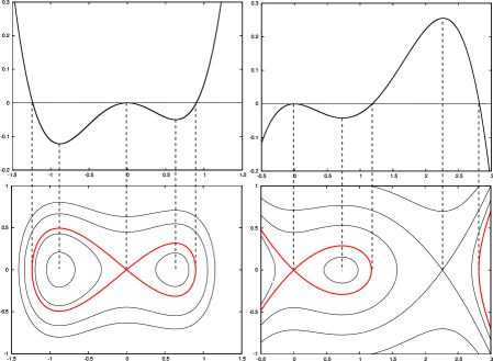
Figure 1. Graph of $F$ and level curves of $I$ with $p(v)=-v+av^{2}+bv^{3}$ for fixed speed $c=\frac{2}{3}$ for $a=\frac{1}{4},$ $b=1$ (left), and $a=2,$ $b=-\frac{1}{3}$ (right).

Solitary waves thus occur in families ${}^{c}V$ parametrized by their speed $c$. The key tool for stability considerations is the so-called moment of instability,

$$m(c) =\int_{-\infty}^{\infty}(^{c}V^{\prime})^{2}\;dx,$$

and our proofs of Theorems 2, 4, and 5 are based on the following fact.

Lemma 0.

The solitary wave ${}^{c}V$ is stable [unstable] if and only if the second derivative

$$m^{\prime\prime}(c)$$

of the moment at the respective speed $c$ is positive [negative].

For this fact and the underlying theory, we refer the reader to [3, 2, 11, 6].

Proof of Theorem 2

Heimburg-Jackson pulses (with $a>0$) are positive. As in [6], we obtain

$$m(c) =\int_{-\infty}^{\infty}(^{c}V^{\prime})^{2}\;dx=2\int_{0}^{\bar{v}(c)}(-2F(v,c))^{1/2}\;dv$$

$$=4\int_{0}^{\sqrt{\bar{v}(c)}}(-2F(\bar{v}(c)-w^{2},c))^{1/2}\;w\;dw,\quad\text{with }w:=(\bar{v}(c)-v)^{1/2}.$$

Differentiating twice yields

(9) $$m^{\prime\prime}(c)=2\int_{0}^{\bar{v}(c)}\frac{v\bigl{(}2F(v,c)(v+2c\bar{v}^{\prime}(c))-cv(F_{v}(v,c)\bar{v}^{\prime}(c)+F_{c}(v,c))\bigr{)}}{(-2F(v,c))^{3/2}}\;dv$$

with

$$F(v,c) =\frac{1}{2}(c^{2}-1)v^{2}+\frac{a}{3}v^{3}+\frac{b}{4}v^{4},$$

$$F_{v}(v,c) =(c^{2}-1)v+av^{2}+bv^{3}=c^{2}v+p(v),$$

$$F_{c}(v,c) =cv^{2},$$

$$\bar{v}^{\prime}(c) =-\frac{F_{c}(\bar{v}(c),c)}{F_{v}(\bar{v}(c),c)}.$$

It is not difficult to verify that positivity of the integrand in (9) is equivalent to positivity of

$$Q(v):=\frac{b}{2}v^{3}+\frac{2}{3}av^{2}-v+c\bar{v}^{\prime}(c)\left(c^{2}-1+\frac{1}{3}av\right).$$

Now, one easily checks that

$$Q(\bar{v}(c))=0\quad\hbox{and}\quad Q^{\prime}(v)<-\left(1+\frac{8}{27}\frac{a^{2}}{b}\right)\ \hbox{for all }v\in{\mathbb{R}}.$$

This implies that $Q$ is indeed positive on the interval $(0,\bar{v}(c))$ and thus that $m^{\prime\prime}(c)>0$.

Proof of Theorem 3

Equation (3) is linearly wellposed at constant states $v_{0}\in{\mathbb{R}}$ if and only if every solution of the form $w(x,t)=\exp\left(\lambda t+i\omega x\right),$ $\omega\in{\mathbb{R}},\lambda\in{\mathbb{C}},$ of its linearization

$$w_{tt}+p^{\prime}(v_{0})w_{xx}+w_{xxxx}=0$$

has $\operatorname{Re}\lambda\leq 0.$ Since for any such mode $w$,

$$\lambda^{2}-p^{\prime}(v_{0})\omega^{2}+\omega^{4}=0,$$

this is characterized by $p^{\prime}(v_{0})\equiv-1+2av_{0}+3bv_{0}^{2}\leq 0.$ $p^{\prime}$ has no real zeros iff (5) holds.

Proof of Theorem 4

Here, we have to consider two different cases. Consider first the case of a positive wave. Instability of standing waves and hence ’slow’ly traveling waves follows from the following observation: At $c=0,$

(10) $$m^{\prime\prime}(0)=4\int_{0}^{\bar{v}(0)}\frac{v^{2}F(v,0)}{(-2F(v,0))^{3/2}}\;dv<0,$$

since $F(.,c)<0$ in the intervall $(0,\bar{v}(c)).$ Continuity of integral and integrand implies then stability of waves with speed $c^{2}\approx 0;$ this observation is actually a special case of [7]. On the other hand, to prove stability of ’fast’ waves, we apply Theorem 4 in [6]; translated into the present situation, this theorem guarantees existence of a $c^{*}\in(0,1)$ such that all solitary waves of speed $c^{2}\in(c^{*2},1)$ are stable, provided that $p^{\prime}(0)<0$ and $p^{\prime\prime}(0)>0;$ with

$$p^{\prime}(0)=-1\quad\text{and}\quad p^{\prime\prime}(0)=2a,$$

this is obviously satisfied.
Consider now the case of a negative solitary wave, i.e., $b>0$ and $\underline{v}(c)=\min\,^{c}V<0.$ The considerations for $c^{2}\lesssim 1$ slightly change as the moment of instability is now

$$m(c)=\int_{-\infty}^{\infty}(^{c}V^{\prime})^{2}\;dx=2\int_{0}^{\bar{v}(c)}\left(-2G(v,c)\right)^{1/2}\;dv\quad\hbox{ with now }\bar{v}(c):=-\underline{v}(c)$$

and

$$G(v,c)=F(-v,c)=\frac{1}{2}(c^{2}-1)v^{2}-\frac{a}{3}v^{3}+\frac{b}{4}v^{4},$$

and its second derivative is (9) with $F$ and its derivatives replaced by $G$ and its derivatives. An obvious analogue of relation (10) keeps implying instability of waves with speed close to $0$. The following observation now shows instability of ’fast’ waves with speed $c^{2}\lesssim 1.$ The quantities $\bar{v}=-\underline{v},m,m^{\prime\prime}$ extend to the limiting value $c^{2}=1$, with $\bar{v}(\pm 1)=(4a)/(3b)$ and $\bar{v}^{\prime}(\pm 1)=-3/a$. Thus, for all $v\in(0,\bar{v}(\pm 1))$,

$$\operatorname{sgn}m^{\prime\prime}(\pm 1) =\operatorname{sgn}v\left(2G(v,1)\left(v+2\bar{v}^{\prime}(1)\right)-v\left(G_{v}(v,1)\bar{v}^{\prime}(1)+G_{c}(v,1)\right)\right)$$

$$=\operatorname{sgn}\left(\frac{-2a}{3}+\frac{b}{2}v\right)$$

$$<0.$$

Now by continuity of integral and integrand this implies $m^{\prime\prime}(c)<0$ for $c^{2}\lesssim 1.$ (Note in passing that in this case the minimum of the wave, and thus the wave’s amplitude, do not tend to zero for $c^{2}\to 1$).

As can be seen in Figure 2, stable negative waves occur when $k=b/a^{2}$ is large enough.

3. Proof of Theorem 5 and plots of sgn$(m^{\prime\prime}(c))$

We turn from estimating $m^{\prime\prime}(c)$ to evaluating this quantity. Let

$$g(k,c) :=\arcsin\left(\frac{2}{3}\frac{1}{\sqrt{\frac{4}{9}+2k(1-c^{2})}}\right),$$

$$\tilde{g}(k,c) :=-\ln\left(-\frac{\sqrt{\frac{4}{9}+2k(1-c^{2})}}{-\frac{2}{3}+\sqrt{-2k(1-c^{2})}}\right),$$

and

$$h(k,c):=\frac{4\left(18kc^{2}-2-9k\right)\sqrt{1-c^{2}}}{k\left(2+9k(1-c^{2})\right)}.$$

Proposition 0.

If $a>0$, the following holds with $k=b/a^{2}$.
(i) In the case of $b>0$ and a positive wave, the assertion of Theorem 5 holds with

$$\mu(a,b,c)=h(k,c)-\frac{4}{3k}\sqrt{\frac{2}{k}}\left(g(k,c)-\frac{\pi}{2}\right).$$

(ii) In the case of $b>0$ and a negative wave, the assertion of Theorem 5 holds with

$$\mu(a,b,c)=h(k,c)-\frac{4}{3k}\sqrt{\frac{2}{k}}\;\left(g(k,c)+\frac{\pi}{2}\right).$$

(iii) In the case of $b<0$ and a positive wave, the assertion of Theorem 5 holds with

$$\mu(a,b,c)=h(k,c)-\frac{4}{3k}\sqrt{-\frac{2}{k}}\tilde{g}(k,c).$$

Remark. Note that with $a>0$, there are no negative solitary waves in the case $b<0$. We refrain from formulating the obvious analogue of Proposition 1 for the case $a<0$.

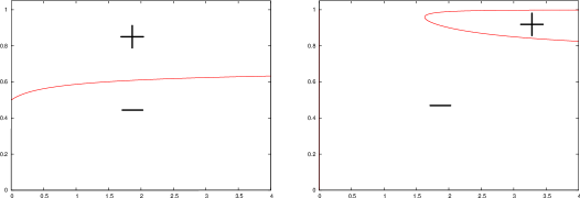
Figure 2. Plot of $m^{\prime\prime}=0$ in the case $a,b>0$ for positive (left) and negative (right) waves. The horizontal axis is $k={b}/{a^{2}}$ and the vertical axis is $c$. The $\pm$ signs refer to regions where $m^{\prime\prime}\gtrless 0.$

Proof.

As cases (ii) and (iii) can be treated analogously, we consider only case (i). By elementary integration, we obtain

$$m(c) =2\int_{0}^{\bar{v}(c)}(-2F(v,c))^{1/2}\;dv$$

$$=2\int_{0}^{\bar{v}(c)}v\left(-\frac{b}{2}v^{2}-\frac{2}{3}av+1-c^{2}\right)^{1/2}\;dv$$

$$=\frac{a}{3b^{2}}\left(2b(1-c^{2})+\frac{4}{9}a^{2}\right)\sqrt{\frac{2}{b}}\arcsin\left(\frac{-bv-\frac{2}{3}a}{\left(\frac{4}{9}a^{2}+2b(1-c^{2})\right)}\right)\Bigg{|}_{v=0}^{v=\bar{v}(c)}\;+$$

$$+\frac{4}{3b}(1-c^{2})^{3/2}+\frac{4a}{9b^{2}}(1-c^{2})^{1/2}.$$

After some slightly tedious calculations, this yields

$$m^{\prime\prime}(c) =\frac{4\left(18kc^{2}-2-9k\right)\sqrt{1-c^{2}}}{k\left(2+9k(1-c^{2})\right)}-\frac{4}{3k}\sqrt{\frac{2}{k}}\left(\arcsin\left(\frac{2}{3}\frac{1}{\sqrt{\frac{4}{9}+2k(1-c^{2})}}\right)-\frac{\pi}{2}\right).$$

∎

References

- [1] R. Appali, U. van Rienen, T. Heimburg, A comparison of the Hodgkin-Huxley model and the soliton theory for the action potential in nerves, in: Aleš Iglič (Editor) Advances in planar lipid bilayers and liposomes vol. 16 (2012), 275–299.
- [2] J. Bona, L. Sachs, Global existence of smooth solutions and stability of solitary waves for a generalized Boussinesq Equation, Comm. Math. Phys. 118 (1988), 15–29.
- [3] M. Grillakis, J. Shatah, W. Strauss, Stability theory of solitary waves in the presence of symmetry, I, J. Funct. Anal. 74 (1987), 160–197.
- [4] R. Grimshaw, D. Pelinovsky, E. Pelinovsky, A. Slunyaev, Generation of large-amplitude solitons in the extended Korteweg-de Vries equation. Chaos 12 (2002), 1070–1076.
- [5] T. Heimburg, A. D. Jackson, On soliton propagation in biomembranes and nerves, PNAS 251 (2005), 9790–9795.
- [6] J. Höwing, Stability of large- and small-amplitude solitary waves in the generalized Korteweg–de Vries and Euler–Korteweg/Boussinesq equations, J. Differential Equations 251 (2011), 2515–2533.
- [7] J. Höwing, Standing solitary Euler-Korteweg waves are unstable, http://arxiv.org/abs/1301.2767.
- [8] C. K. R. T. Jones, Stability of the travelling wave solution of the FitzHugh-Nagumo system. Trans. Amer. Math. Soc. 286 (1984), 431–469.
- [9] M. Krupa, B. Sandstede, P. Szmolyan, Fast and slow waves in the FitzHugh-Nagumo equation. J. Differential Equations 133 (1997), 49–97.
- [10] B. Lautrup, R. Appali, A. D. Jackson, T. Heimburg, The stability of solitons in biomembranes and nerves, Eur. Phys. J. E 34 (2011), 9 pages.
- [11] K. Zumbrun, A sharp stability criterion for soliton-type propagating phase boundaries in Korteweg’s model, Z. Anal. Anwend. 27 (2008), 11–30.