Observer-Based Higher Order Sliding Mode Control of Unity Power Factor in Three-Phase AC/DC Converter for Hybrid Electric Vehicle Applications

Abstract

In this paper, a full-bridge boost power converter topology is studied for power factor control, using output higher order sliding mode control. The AC/DC converters are used for charging the battery and super-capacitor in hybrid electric vehicles from the utility. The proposed control forces the input currents to track the desired values, which can controls the output voltage while keeping the power factor close to one. Super-twisting sliding mode observer is employed to estimate the input currents and load resistance only from the measurement of output voltage. Lyapunov analysis shows the asymptotic convergence of the closed loop system to zero. Simulation results show the effectiveness and robustness of the proposed controller.

1 INTRODUCTION

With the advent of distributed DC power sources in the energy sector, the use of boost type three phase rectifiers has increased in industrial applications, especially, battery charger in hybrid electric vehicles (HEV) (Egan et al., 2007; Pahlevaninezhad et al., 2012a, b; Kuperman et al., 2012). Power-factor-corrected utility interfaces are of great importance in the HEV industry. The complete energy conversion cycle of the HEV must convert electrical power from the utility to mechanical power at the drive axle as efficiently and as economically as possible (Egan et al., 2007; Guerrero et al., 2013; Liu et al., 2013). Different power conversion systems of plug-in HEV power conditioning systems are presented in Cao and Emadi (2009); Lee et al. (2009); Wirasingha and Emadi (2011); Camara et al. (2010); Amjadi and Williamson (2010).

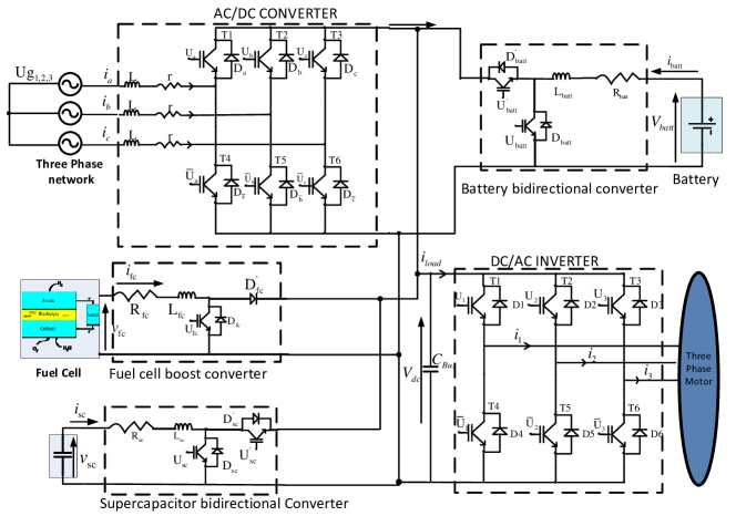
Fig. 1 shows the structure of the hybrid electric vehicle power conversion system, which consists of of an AC/DC converter, a three phase DC/AC inverter (Zhong and Hornik, 2013; Hornik and Zhong, 2013), three DC/DC converters and various power storages i.e. source grid, battery, super-capacitor and fuel cell. The AC/DC converter is used to charge the battery and super-capacitor through its bidirectional DC/DC converters, while ensuring that the utility current is drawn at unity power factor in order to minimize line distortion and maximize the real power available from the utility outlet. The battery and super-capacitor supply power to the three-phase inverter which feeds the three-phase motor.

The AC/DC converter consists of two stages (Emadi et al., 2008; Hayes et al., 1999). The first stage is Power Factor Correction (PFC), which simultaneously regulates the DC-link voltage level and the line current waveform. The second stage is a charger with different types of resonant or pulse-width-modulation (PWM) DC/DC converters (Egan et al., 2007). PFC is used to improve the quality of the input phase current that is sourced from the utility by generating and tracking the desired current profile while the charger is used to charge the battery and super-capacitor in a HEV.

Many schemes and solutions are proposed in the field of PFC. Linear control methods using linear regulators for the output voltage control have been proposed in Pan and Chen (1993); Dixon and Ooi (1988), which change the modulation index slowly, thus resulting in a slow dynamical response. Consequently, the linear feedback control of the rectifier output voltage becomes slow and difficult. Moreover, due to coupling between the duty-cycle and the state variables in the AC/DC boost converter, linear controllers are not able to perform optimally for the whole range of operating conditions. In contrast with linear control, nonlinear approaches can optimize the performance of the AC/DC converter over a wide range of operating conditions. Many nonlinear techniques have been proposed, such as input-output linearization (Lee, 2003), feedback linearization (Lee et al., 2000), fuzzy logic control (Cecati et al., 2005), passivity-based control (Escobar et al., 2001), back-stepping technique control (Allag et al., 2007), Lyapunov-based control (Pahlevaninezhad et al., 2012a; Kömürcügil and Kükrer, 1998), differential flatness based control (Pahlevaninezhad et al., 2012b; Houari et al., 2012; Thounthong, 2012), and sliding mode control (Shtessel et al., 2008; Silva, 1999; Tan et al., 2007). However, most of the above works need continuous measurements of AC voltages, AC currents and DC voltage. This requires a large number of both voltage and current sensors, which increases system complexity, cost, space, and reduces system reliability. Moreover, the sensors are susceptible to electrical noise, which cannot be avoided during high-power switching. Reducing the number of sensors has a significant affect upon the control system’s performance. A few results have been proposed to reduce the current sensors (Andersen et al., 1999; Pan and Chen, 1993; Lee and Lim, 2002; Lee et al., 2001) where the input phase currents are reconstructed from the switching states of the AC/DC rectifier and the measured DC-link currents, and then used in feedback control. However, they require digital sampling of the DC-link current in every switching cycle and numerical computations. The accuracy of measurement is inherently controlled by the sampling rate.

The objective of this paper is to design an efficient AC/DC power converter that charges the battery and super-capacitor in a HEV with unity power factor, by eliminating the using of current sensors. Only voltage sensors are required for measuring the output voltage and source voltage. A Super-Twisting (ST) Sliding Mode Observer (SMO) is designed to observe the phase currents and load resistance (Shtessel et al., 2008; Pu et al., 2012) from the measured output voltage. The proposed ST SMO guarantees fast convergence rate of the observation error dynamics, facilitating the design of controllers. The controller and observer design is based on the two goals mentioned in Vadim Utkin, Jurgen Guldner, Jingxin Shi (2009); Edwards and Spurgeon (1998), for the design of an efficient AC/DC power converter: 1) Unity power factor to maximize the performance of the power conversion. 2) Ripple free output voltage.

Sliding mode algorithm is known for the characteristics of robustness and effectiveness (Edwards and Spurgeon, 1998), making it an effective method to deal with the nonlinear behavior of the boost rectifiers. The ST Sliding Mode Control (SMC) allows not only the achievement of the high performance of the system but also the maintenance of the functionality under parametric uncertainty and external disturbance. A strong Lyapunov function is introduced to prove the stability of both the observer and controller system.

The paper is organized as follows. In Section II, the mathematical model and control objectives are presented. In Section III, the design of observer-based current controller based on ST Algorithm (STA) is presented. In Section IV, we show the design of the parameter observer for the system, and power factor is also estimated. In Section V, simulations results of the performance of the obtained ST SMC compared with the conventional PI controller are presented. Finally, some conclusions are drawn in Section VI.

Figure 1: PEMFC powered hybrid system consists of Source Grid, Fuel Cell, Super-capacitor and battery

2 PROBLEM FORMULATION

2.1 System Modeling

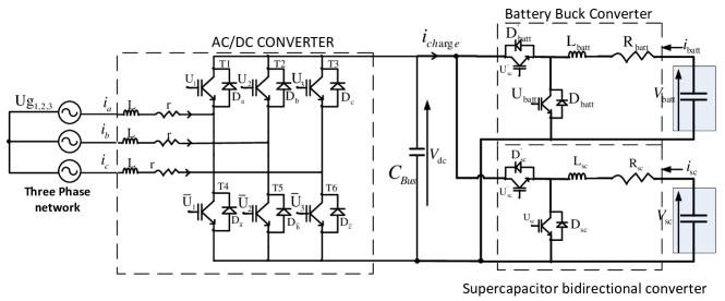
The power circuit of the three phase voltage source AC/DC full-bridge boost converter under consideration is shown in Fig. 2. It is assumed that a equivalent resistive load $\displaystyle R_{L}$ is connected to the output of the AC/DC converter (Pahlevaninezhad et al., 2012a, b).

Figure 2: Electrical circuit of the three phase AC/DC boost converter

The control inputs, as they appear in the system, are defined as $\displaystyle\bm{u}=[u_{1}\ \ u_{2}\ \ u_{3}]^{T}$, which take values from the discrete set $\displaystyle\{-1,+1\}$. The corresponding inverse control $\displaystyle\bm{\bar{u}}=[\bar{u}_{1}\ \ \bar{u}_{2}\ \ \bar{u}_{3}]^{T}$ takes the opposite values at the same time, i.e. $\displaystyle u_{1}=+1$ means $\displaystyle\bar{u}_{1}=-1$ which corresponds to the conducting state for the upper switching element $\displaystyle T_{1}$ and nonconducting state for the bottom switching element $\displaystyle T_{4}$ (Shtessel et al., 2008).

The mathematical model of the boost AC/DC converter in phase coordinate frame can be obtained through analyzing the circuit (Pan and Chen, 1993),

$$\left\{\begin{split}\frac{di_{a}}{dt}=&-\frac{r}{L}i_{a}-\frac{U_{0}}{6L}(2u_{1}-u_{2}-u_{3})+\frac{1}{L}U_{g_{1}},\\ \frac{di_{b}}{dt}=&-\frac{r}{L}i_{b}-\frac{U_{0}}{6L}(2u_{2}-u_{1}-u_{3})+\frac{1}{L}U_{g_{2}},\\ \frac{di_{c}}{dt}=&-\frac{r}{L}i_{c}-\frac{U_{0}}{6L}(2u_{3}-u_{1}-u_{2})+\frac{1}{L}U_{g_{3}},\\ \frac{dU_{0}}{dt}=&-\frac{U_{0}}{R_{L}C}+\frac{1}{2C}(i_{a}u_{1}+i_{b}u_{2}+i_{c}u_{3}).\end{split}\right.$$ (1)

It can also be written as,

$$\left\{\begin{split}\frac{\bm{di}}{\bm{dt}}=&-\frac{r}{L}\bm{i}-\frac{U_{0}}{6L}B\bm{u}+\frac{1}{L}\bm{U_{g}},\\ \frac{dU_{0}}{dt}=&-\frac{U_{0}}{R_{L}C}+\frac{1}{2C}\bm{u}^{T}\bm{i}.\end{split}\right.$$ (2)

where $\displaystyle r$ is parasitic phase resistance (including voltage source internal resistance and impedance of switching elements in open state); $\displaystyle R_{L}$ is the load resistance; $\displaystyle L$ is phase inductor; $\displaystyle C$ is output capacitor; $\displaystyle U_{0}$ is output voltage; $\displaystyle\bm{i}=\begin{bmatrix}i_{a}&i_{b}&i_{c}\end{bmatrix}^{T}$ are the input phase currents; $\displaystyle\bm{U_{g}}=\begin{bmatrix}U_{g_{1}}&U_{g_{2}}&U_{g_{3}}\end{bmatrix}^{T}$ are the source voltages which have different magnitudes but the same frequency and phase shift of $\displaystyle\frac{2\pi}{3}$ electrical degrees (with respect to each other); and $\displaystyle\bm{u}=\begin{bmatrix}u_{1}&u_{2}&u_{3}\end{bmatrix}^{T}$ are control signals. The gain matrix and source voltage are as follows,

$$B=\begin{bmatrix}2&-1&-1\\ -1&2&-1\\ -1&-1&2\end{bmatrix},\ \ \bm{U_{g}}=E\begin{bmatrix}sin(\theta)\\ sin(\theta-\frac{2}{3}\pi)\\ sin(\theta+\frac{2}{3}\pi)\end{bmatrix}$$ (3)

where $\displaystyle E$ is the magnitude of the source voltages (Kömürcügil and Kükrer, 1998).

For modeling and control design, it is convenient to transform three-phase variables into a rotating $\displaystyle(d,q)$ frame. The transformed variables is defined as,

$$\begin{split}\bm{u_{dq}}=&\begin{bmatrix}u_{d}\\ u_{q}\end{bmatrix}=T\bm{u},\ \ \bm{i_{dq}}=\begin{bmatrix}i_{d}\\ i_{q}\end{bmatrix}=T\bm{i},\\ T\bm{U_{g}}=&\begin{bmatrix}U_{g_{d}}\\ U_{g_{q}}\end{bmatrix}.\end{split}$$ (4)

where

$$T=\frac{2}{3}\begin{bmatrix}cos(\omega t)&cos(\omega t-\frac{2}{3}\pi)&cos(\omega t+\frac{2}{3}\pi)\\ sin(\omega t)&sin(\omega t-\frac{2}{3}\pi)&sin(\omega t+\frac{2}{3}\pi)\end{bmatrix}$$ (5)

is the Park’s transformation Bose (2002); Lee (2003).

From (3) and (5), it follows that $\displaystyle U_{g_{d}}=0$ and $\displaystyle U_{g_{q}}=E$. The dynamical model of the AC/DC converter in the rotating $\displaystyle(d,q)$ frame can be expressed as (Kömürcügil and Kükrer, 1998; Lee et al., 2000; Silva, 1997)

$$\left\{\begin{split}\frac{di_{d}}{dt}=&-\frac{r}{L}i_{d}+\omega i_{q}-\frac{U_{0}}{2L}u_{d},\\ \frac{di_{q}}{dt}=&-\frac{r}{L}i_{q}+\frac{E}{L}-\omega i_{d}-\frac{U_{0}}{2L}u_{q},\\ \frac{dU_{0}}{dt}=&-\frac{U_{0}}{R_{L}C}+\frac{3(i_{d}u_{d}+i_{q}u_{q})}{4C}.\end{split}\right.$$ (6)

where $\displaystyle\omega$ is the angular frequency of the source voltage. In the transformed state equation (6), the state vector is defined as $\displaystyle\bm{x}=\begin{bmatrix}x_{1}&x_{2}&x_{3}\end{bmatrix}^{T}=\begin{bmatrix}i_{d}&i_{q}&U_{0}\end{bmatrix}^{T}$ and the control input vector $\displaystyle\bm{u_{dq}}=\begin{bmatrix}u_{d}&u_{q}\end{bmatrix}^{T}$ are the switching functions $\displaystyle\bm{u}=\begin{bmatrix}u_{1}&u_{2}&u_{3}\end{bmatrix}^{T}$ in synchronously rotating $\displaystyle(d,q)$ coordinate. From the control point of view, the model of AC/DC converter in $\displaystyle(d,q)$ frame has the advantage of reducing the current control task into a set-point tracking problem (Lee, 2003).

2.2 Control Objectives

Assumption 1

The phase voltage $\displaystyle\bm{U_{g}}$ and output voltage $\displaystyle U_{0}$ are measurable;

The control objectives are as follows,

• The input phase currents $\displaystyle i_{a},i_{b},i_{c}$ should be in phase with corresponding input source voltage $\displaystyle U_{g_{1}},U_{g_{2}},U_{g_{3}}$ in order to obtain a unity power factor.

• The DC component of the output voltage should be driven to some desired value $\displaystyle{U^{*}_{0}}$ while its AC component has to be attenuated to a given level.

3 OBSERVER-BASED SLIDING MODE CONTROLLER DESIGN

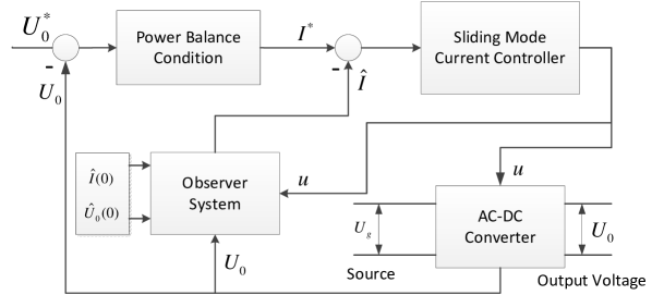
In observer-based sliding mode control, the real plant states are substituted by observer states, reducing the number of measurements. It has been shown that the performance of an observer-based sliding mode controller can be improved significantly by keeping the plant system and the observer system operating closely (Sira-Ramirez et al., 1996). Fig. 3 shows the structure of the observer-based control system for three phase AC/DC converters, which consists of two important parts: sliding mode current observer and controller system.

Figure 3: Observer-Based Control Structure of a Three Phase AC/DC Converter

3.1 Super-Twisting Sliding Mode Observer Design

The proposed observer is designed in the following two steps,

1. Analyzing the observability of the nonlinear system;

2. Construction of the ST Observer;

3.1.1 Observability Analysis of the System

In order to construct an observer for a system, it is necessary to verify the observability of the system i.e. there exists the possibility of obtaining the states of a system only from the knowledge of its inputs and outputs up to time $\displaystyle t$ (Besançon, 2007). Considering the following nonlinear system,

$$\left\{\begin{split}\dot{\bm{x}}=&\bm{f_{u}}(\bm{x},\bm{u}),\\ \bm{y}=&\begin{bmatrix}h_{1}(x)&\cdots&h_{p}(x)\end{bmatrix}^{T}.\end{split}\right.$$ (7)

where $\displaystyle\bm{x}\in\mathbb{R}^{n}$ are the state vectors, $\displaystyle\bm{u}\in\mathbb{R}^{m}$ are the bounded inputs, $\displaystyle\bm{y}\in\mathbb{R}^{p}$ are the outputs. Assume that the vector field $\displaystyle\bm{f_{u}}(\cdot,\cdot)$ is a sufficiently smooth function.

Definition 1

(Hermann and Krener, 1977) The system described by (7) is locally observable if the matrix defined by (8) satisfies observability rank condition $\displaystyle dim(\mathrm{O})=n$ at a point $\displaystyle x_{0}$,

$$\begin{split}\mathrm{O}=&\begin{bmatrix}dL^{0}_{f_{u}}(h_{1})&dL^{0}_{f_{u}}(h_{2})&\cdots&dL^{0}_{f_{u}}(h_{p})\\ dL^{1}_{f_{u}}(h_{1})&dL^{1}_{f_{u}}(h_{2})&\cdots&dL^{1}_{f_{u}}(h_{p})\\ \vdots&\vdots&\ddots&\vdots\\ dL^{n-1}_{f_{u}}(h_{1})&dL^{n-1}_{f_{u}}(h_{2})&\cdots&dL^{n-1}_{f_{u}}(h_{p})\end{bmatrix},\end{split}$$ (8)

where $\displaystyle L_{f_{u}}(h)$ denotes the Lie derivative of $\displaystyle h$ with respect to $\displaystyle f_{u}$.

Taking the output as $\displaystyle y=x_{3}=U_{0}$, the application of Definition 1 leads to the following observability matrix,

$$\mathrm{O}=\begin{bmatrix}0&0&1\\ \frac{3u_{d}}{4C}&\frac{3u_{q}}{4C}&-\frac{1}{RC}\\ -\varrho u_{d}-\frac{3\omega u_{q}}{4C}&\frac{3\omega u_{d}}{4C}-\varrho u_{q}&-\frac{3\|u_{dq}\|^{2}}{8LC}+(\frac{1}{R_{L}C})^{2}\end{bmatrix},$$ (9)

where $\displaystyle\varrho=\frac{3}{4C}(\frac{r}{L}+\frac{1}{R_{L}C})$, and $\displaystyle\|u_{dq}\|^{2}_{2}=u^{2}_{d}+u^{2}_{q}$. Thus, it is possible to observe the currents $\displaystyle i_{d},i_{q}$ from the measurement of the output voltage $\displaystyle U_{0}$ when $\displaystyle\|u_{dq}\|_{2}\neq 0$. In the case of singular inputs $\displaystyle u_{d}=0,u_{q}=0$ which results the system (6) into a reduced system with detectability property. This property allows to construct an open-loop observer (Besançon, 2007; Sarinana et al., 2000).

3.1.2 Construction of the Nonlinear Observer

Assume that the only measured variable is the output DC voltage, i.e. $\displaystyle y=x_{3}=U_{0}$. Thus, a ST SMO for (6) is constructed as follows

$$\left\{\begin{split}\frac{d\hat{i}_{d}}{dt}=&-\frac{r}{L}\hat{i}_{d}+\omega\hat{i}_{q}-\frac{{U}_{0}}{2L}u_{d}+k_{1}\mu(e_{3}),\\ \frac{d\hat{i}_{q}}{dt}=&-\frac{r}{L}\hat{i}_{q}-\omega\hat{i}_{d}-\frac{{U}_{0}}{2L}u_{q}+\frac{E}{L}+k_{2}\mu(e_{3}),\\ \frac{d\hat{U}_{0}}{dt}=&-\frac{U_{0}}{R_{L}C}+\frac{3}{4C}(\hat{i}_{d}u_{d}+\hat{i}_{q}u_{q})+\mu(e_{3}).\end{split}\right.$$ (10)

where the observation errors and STA are defined as

$$\begin{split}e_{1}&=i_{d}-\hat{i}_{d},e_{2}=i_{q}-\hat{i}_{q},e_{3}=U_{0}-\hat{U}_{0},\\ \mu(e_{3})&=\lambda|e_{3}|^{\frac{1}{2}}sign(e_{3})+\alpha\int_{0}^{t}sign(e_{3})d\tau,\end{split}$$ (11)

with some positive constants $\displaystyle\lambda,\alpha$ respectively.

Then the error dynamics is given by

$$\displaystyle\dot{e}_{1} \displaystyle= \displaystyle-\frac{r}{L}e_{1}+\omega e_{2}-k_{1}\mu(e_{3}),$$ (12)

$$\displaystyle\dot{e}_{2} \displaystyle= \displaystyle-\omega e_{1}-\frac{r}{L}e_{2}-k_{2}\mu(e_{3}),$$ (13)

$$\displaystyle\dot{e}_{3} \displaystyle= \displaystyle\frac{3}{4C}(u_{d}e_{1}+u_{q}e_{2})-\mu(e_{3}).$$ (14)

where $\displaystyle\mu(e_{3})$ is the same as in equation (11).

The design problem is transformed into determining $\displaystyle\alpha,\lambda$ and $\displaystyle k_{1},k_{2}$ which are the tuning parameters to ensure the convergence of the error system (12,13, 14).

Proposition 3.1.

Consider the system (14), and assume that the control inputs are bounded,

$$\|\bm{u_{dq}}\|_{2}\leq\sqrt{2},$$ (15)

Then, the trajectories of the system (14) converge to zero in finite time, and the resulting reduced order dynamics (12,13) are exponentially stable, if the gains $\displaystyle\alpha,\lambda$ of the STA and tuning parameters $\displaystyle k_{1},k_{2}$ are chosen as Levant (1998),

$$\begin{split}\alpha>&F,\quad\lambda^{2}>\alpha,\end{split}$$ (16)

$$\begin{split}k_{1}=&\begin{cases}\kappa u_{d},\ \ \quad if\ \ |e_{3}|=0\\ 0.\ \ \quad\quad else\end{cases},\\ k_{2}=&\begin{cases}\kappa u_{q},\ \ \quad if\ \ |e_{3}|=0\\ 0.\ \ \quad\quad else\end{cases}\end{split}$$ (17)

where $\displaystyle F$ and $\displaystyle\kappa$ are some positive constants.

Proof 3.2.

The proof is divided into two steps. In the first step, the equation (14) is proven to be finite time stable. Then, the resulting reduced order dynamics (12,13) are proven to be exponentially stable with faster convergence rate than its open loop dynamics (detectability property). At the beginning, the two correction gains $\displaystyle k_{1},k_{2}$ are zero due to $\displaystyle e_{3}\neq 0$. The system (12,13) becomes

$$\begin{bmatrix}\dot{e}_{1}\\ \dot{e}_{2}\end{bmatrix}=\underbrace{\begin{bmatrix}-\frac{r}{L}&\omega\\ -\omega&-\frac{r}{L}\end{bmatrix}}_{A}\begin{bmatrix}{e}_{1}\\ {e}_{2}\end{bmatrix}$$ (18)

It is easy to conclude that the system (18) is exponentially stable given that $\displaystyle A$ is a Hurwitz matrix. Consequently, we can conclude that $\displaystyle e_{1},e_{2},\dot{e}_{1},\dot{e}_{2}$ are bounded

$$\begin{split}|e_{1}(t)|\leq&|e_{1}(0)|,\ \ |e_{2}(t)|\leq|e_{2}(0)|,\\ |\dot{e}_{1}(t)|\leq&\frac{r}{L}|e_{1}(t_{0})|+\omega|e_{2}(t_{0})|,\\ |\dot{e}_{2}(t)|\leq&\omega|e_{1}(t_{0})|+\frac{r}{L}|e_{2}(t_{0})|.\end{split}$$ (19)

The condition of (15) is deduced from the Park transformation (4) and the control inputs $\displaystyle\bm{u}$ which take values from the discrete set $\displaystyle\{-1,+1\}$,

$$\begin{split}\|\bm{u_{dq}}\|_{2}\leq&\|T\|_{2}\|\bm{u}\|_{2}=\sqrt{\lambda_{max}(T^{T}T)}\|\bm{u}\|_{2}\\ \leq&\sqrt{\frac{2}{3}}\sqrt{3}=\sqrt{2},\end{split}$$ (20)

The equation (14) can be rewritten as,

$$\left\{\begin{split}\dot{e}_{3}=&-\lambda|e_{3}|^{\frac{1}{2}}sign(e_{3})+\varphi,\\ \dot{\varphi}=&-\alpha sign(e_{3})+g(e_{1},e_{2},u_{d},u_{q}),\end{split}\right.$$ (21)

where $\displaystyle g(e_{1},e_{2},u_{d},u_{q})=\frac{3}{4C}\frac{d}{dt}(u_{d}e_{1}(t)+u_{q}e_{2}(t))$ is considered as a bounded decreasing perturbation.

It follows from (19, 20) that $\displaystyle\left|g\right|\leq F$, with a positive value $\displaystyle F$. Given that the gains of the STA are chosen as (16), $\displaystyle e_{3},\dot{e}_{3}$ converge to zero in finite time (Levant, 1998).

Thereafter, the equivalent output-error injection $\displaystyle\mu(e_{3})$ in (14) can be obtained directly without any low pass filters,

$$\mu(e_{3})=\frac{3}{4C}(u_{d}e_{1}+u_{q}e_{2}),$$ (22)

When the sliding motion takes place ($\displaystyle e_{3}=0,\dot{e}_{3}=0$), the gains $\displaystyle k_{1},k_{2}$ will switch according to (17). Then, the equivalent injection (22) is substituted into the system (12,13) in order to get the reduced order dynamics,

$$\begin{bmatrix}\dot{e}_{1}\\ \dot{e}_{2}\end{bmatrix}=\begin{bmatrix}-\frac{r}{L}&\omega\\ -\omega&-\frac{r}{L}\end{bmatrix}\begin{bmatrix}e_{1}\\ e_{2}\end{bmatrix}-\bar{A}\begin{bmatrix}e_{1}\\ e_{2}\end{bmatrix}$$ (23)

where $\displaystyle\bar{A}=\frac{3\kappa}{4C}\begin{bmatrix}u^{2}_{d}&u_{d}u_{q}\\ u_{d}u_{q}&u^{2}_{q}\end{bmatrix}$.

Consider a candidate Lyapunov function for system (23) as,

$$V(e)=e^{T}Pe,$$ (24)

where $\displaystyle e^{T}=[e_{1},e_{2}]$, and $\displaystyle P=\begin{bmatrix}\frac{L}{2r}&0\\ 0&\frac{L}{2r}\end{bmatrix}$ which satisfies the equation $\displaystyle{A}^{T}P+P{A}=-I$, where $\displaystyle I$ is an identity matrix.

Then, the time derivative of $\displaystyle V$ along the trajectories of system (23) is given by,

$$\begin{split}\dot{V}(e)=&-e^{T}e-e^{T}(\bar{A}^{T}P+P\bar{A})e\\ =&-e^{2}_{1}-e^{2}_{2}-\frac{3\kappa L}{4rC}(u_{d}e_{1}+u_{q}e_{2})^{2}\\ \leq&-e^{2}_{1}-e^{2}_{2},\end{split}$$ (25)

It should be noted from (25) that for any positive $\displaystyle\kappa$, the system (23) is exponentially stable with faster convergence rate compared with the open loop dynamic (18). The proof of the Proposition 3.1 is finished.

In the next Subsection, an output feedback ST current control is designed in order to achieve the objective of unity power factor and ripple free output voltage.

3.2 Output Feedback ST Sliding Mode Current Control

The STA is popular among the Second Order Sliding Mode (SOSM) algorithms because it is a unique absolutely continuous sliding mode algorithm, therefore it does not suffer from the problem of chattering (Levant, 1993, 2007). The main advantages of the ST SMC (Vadim Utkin, Jurgen Guldner, Jingxin Shi, 2009) are as follows:

1. It does not need the evaluation of the time derivative of the sliding variable;

2. Its continuous nature suppresses arbitrary disturbances with bounded time derivatives;

The control objectives are define in the Subsection 2.2.

3.2.1 Desired current calculation with unity power factor

Normally, the value of the inductance $\displaystyle L\ll 1$ in the system (6), and the right-hand sides of the equations in (6) have the values of the same order. Hence $\displaystyle\frac{di_{d}}{dt},\frac{di_{q}}{dt}\gg\frac{dU_{0}}{dt}$, implying that the dynamics of $\displaystyle i_{d}$ and $\displaystyle i_{q}$ are much faster than those of $\displaystyle U_{0}$ (Vadim Utkin, Jurgen Guldner, Jingxin Shi, 2009). Provided that the fast dynamics are stable, based on the singular perturbation theory (Hassan K. Khalil, 2007), let the first and second equations of (6) be zero formally, then $\displaystyle u_{d},u_{q}$ can be obtained,

$$\left\{\begin{split}\frac{U_{0}}{2L}u_{d}=&-\frac{r}{L}i^{*}_{d}+\omega i^{*}_{q},\\ \frac{U_{0}}{2L}u_{q}=&-\frac{r}{L}i^{*}_{q}-\omega i^{*}_{d}+\frac{E}{L},\\ \frac{dU_{0}}{dt}=&-\frac{U_{0}}{R_{L}C}+\frac{3}{4C}(i^{*}_{d}u_{d}+i^{*}_{q}u_{q}).\end{split}\right.$$ (26)

Based on equation (26), the reference currents $\displaystyle i^{*}_{d},i^{*}_{q}$ will be determined depending on the desired system performance. Substitute the first and second equation into the third equation of (26) yields,

$$\frac{dU_{0}}{dt}=-\frac{U_{0}}{R_{L}C}+\frac{3}{2}\frac{i^{*}_{q}E-E_{r}}{U_{0}C},$$ (27)

where $\displaystyle E_{r}=r({i^{*}_{d}}^{2}+{i^{*}_{q}}^{2})$ represents the energy consumed by parasitic phase resistance.

Considering the Power-Balance condition (Kömürcügil and Kükrer, 1998),

$$\frac{3}{2}(i^{*}_{q}E-E_{r})=\frac{U^{*2}_{0}}{R_{L}},$$ (28)

The reference current $\displaystyle i^{*}_{d}$ is set to zero for guaranteeing Unity-Power-Factor which leads to the following calculation of the reference current $\displaystyle i^{*}_{q}$,

$$i^{*}_{q}=\frac{E}{2r}\pm\frac{1}{2}\sqrt{\frac{E^{2}}{r^{2}}-\frac{8U^{*2}_{0}}{3R_{L}r}},$$ (29)

under constraint for desired output voltage $\displaystyle U^{*}_{0}$,

$$U^{*}_{0}\leq E\sqrt{\frac{3R_{L}}{8r}},$$ (30)

Finally, $\displaystyle i^{*}_{d}$ and $\displaystyle i^{*}_{q}$ are obtained as follows (due to minimal energy consumption),

$$\left\{\begin{split}i^{*}_{d}=&0,\\ i^{*}_{q}=&\frac{E}{2r}-\frac{1}{2}\sqrt{\frac{E^{2}}{r^{2}}-\frac{8U^{*2}_{0}}{3R_{L}r}},.\end{split}\right.$$ (31)

As tracking error vector approaches zero, i.e., $\displaystyle i_{d}\rightarrow i^{*}_{d}$ and $\displaystyle i_{q}\rightarrow i^{*}_{q}$, the zero dynamics have the form Lee (2003)

$$\frac{dU_{0}}{dt}=-\frac{U_{0}}{R_{L}C}+\frac{U^{*2}_{0}}{R_{L}CU_{0}},$$ (32)

Define a new variable $\displaystyle Z=U^{2}_{0}$, equation (32) can be rewritten as,

$$\frac{dZ}{dt}=-\frac{2}{R_{L}C}(Z-U^{*2}_{0}),$$ (33)

For a positive initial value of the output voltage, the steady-state value of $\displaystyle U_{0}$ will converge to the desired level $\displaystyle U^{*}_{0}$ with the time constant $\displaystyle\frac{R_{L}C}{2}$ exponentially. Therefore, the tracking of the reference current achieves the regulation of output voltage to the desired value $\displaystyle U^{*}_{0}$ with a unity power factor. In the following Subsection 3.2.2, the design of current control based on STA is proposed.

3.2.2 Output Sliding Mode Current Control

We will now design ST SMC for the system (6) based on the proposed observer (10). The switching variables for the current control are defined as,

$$\left\{\begin{split}s_{d}=&i_{d}^{*}-{i}_{d}=i_{d}^{*}-{\hat{i}}_{d}+\hat{i}_{d}-{i}_{d}=\hat{s}_{d}-e_{1},\\ s_{q}=&i_{q}^{*}-{i}_{q}=i_{q}^{*}-{\hat{i}}_{q}+\hat{i}_{q}-{i}_{q}=\hat{s}_{q}-e_{2}.\end{split}\right.$$ (34)

where $\displaystyle i^{*}_{d}$ and $\displaystyle i^{*}_{q}$ are the desired values of the currents in the $\displaystyle(d,q)$ coordinate frame and $\displaystyle e_{1},e_{2}$ are observation errors defined in (11). The desired value is selected to provide the DC power balance between the input power and the output power.

Taking the first time derivative of $\displaystyle\bm{s_{dq}}=[s_{d},s_{q}]^{T}$ yields,

$$\dot{\bm{s}}_{\bm{dq}}=\begin{bmatrix}\frac{r}{L}{i}_{d}-\omega{i}_{q}\\ \dot{i}^{*}_{q}+\frac{r}{L}{i}_{q}-\frac{E}{L}+\omega{i}_{d}\end{bmatrix}+\frac{U_{0d}}{2L}\begin{bmatrix}u_{d}\\ u_{q}\end{bmatrix},$$ (35)

The equation (35) can be rewritten as,

$$\begin{split}\begin{bmatrix}\dot{s}_{d}\\ \dot{s}_{q}\end{bmatrix}=&\begin{bmatrix}-\frac{r}{L}s_{d}+\omega s_{q}\\ -\omega s_{d}-\frac{r}{L}s_{q}\end{bmatrix}+\begin{bmatrix}F_{d}\\ F_{q}\end{bmatrix}+\frac{U_{0d}}{2L}\begin{bmatrix}u_{d}\\ u_{q}\end{bmatrix},\end{split}$$ (36)

where $\displaystyle F_{d}=-\omega{i}^{*}_{q}$, $\displaystyle F_{q}=\dot{i}^{*}_{q}+\frac{r}{L}{i}^{*}_{q}-\frac{E}{L}$.

The control objective is to force the sliding variable $\displaystyle s_{d},s_{q}$ to zero. Design controls $\displaystyle u_{d},u_{q}$ as follows,

$$\begin{split}\bm{{u}_{dq}}=&\begin{bmatrix}{u}_{d}\\ {u}_{q}\end{bmatrix}=\frac{2L}{U_{0d}}\begin{bmatrix}\frac{r}{L}\hat{s}_{d}-\omega\hat{s}_{q}-\mu(\hat{s}_{d})-F_{d}\\ \omega\hat{s}_{d}+\frac{r}{L}\hat{s}_{q}-\mu(\hat{s}_{q})-F_{q}\end{bmatrix},\end{split}$$ (37)

where $\displaystyle\mu(\hat{s}_{d})$ and $\displaystyle\mu(\hat{s}_{q})$ take the form of (11).

Remark 3.3.

Since the control signals (37) are continuous, Pulse Width Modulation (PWM) technique is used to implement the controller on practical platforms (Sabanovic et al., 2004).

Then, Lyapunov analysis is used to prove the convergence of the system (36) under the controller (37) where observation errors are taken into account.

Theorem 3.4.

The output ST SMC (37) ensures the exponential convergence of the state trajectories of the system (36) to the origin $\displaystyle s_{d}=0$, $\displaystyle s_{q}=0$, if the gains of STA $\displaystyle\mu(\hat{s}_{d}),\mu(\hat{s}_{q})$ satisfy the following conditions (Levant, 1998),

$$\begin{split}\alpha_{d}>&F_{d},\quad\lambda^{2}_{d}>\alpha_{d},\\ \alpha_{q}>&F_{q},\quad\lambda^{2}_{q}>\alpha_{q},\end{split}$$ (38)

where $\displaystyle F_{d}$ and $\displaystyle F_{q}$ are some positive constants.

Proof 3.5.

Substitute the control (37) into system (36) yields,

$$\left\{\begin{split}\dot{\hat{s}}_{d}=&-\mu(\hat{s}_{d})-\frac{r}{L}e_{1}+\omega e_{2}+\dot{e}_{1},\\ \dot{\hat{s}}_{q}=&-\mu(\hat{s}_{q})-\omega e_{1}-\frac{r}{L}e_{2}+\dot{e}_{2}.\end{split}\right.$$ (39)

where $\displaystyle e_{12}^{T}=\begin{bmatrix}e_{1}&e_{2}\end{bmatrix}$ are the observation errors. From the result of Proposition 3.1, $\displaystyle\lim_{t\rightarrow\infty}e_{1}(t)=0$ and $\displaystyle\lim_{t\rightarrow\infty}e_{2}(t)=0$. It follows from (19, 23) that the time derivatives of the terms $\displaystyle-\frac{r}{L}e_{1}+\omega e_{2}+\dot{e}_{1}$ and $\displaystyle-\omega e_{1}-\frac{r}{L}e_{2}+\dot{e}_{2}$ are bounded,

$$\begin{split}&\left|\frac{d}{dt}\left(-\frac{r}{L}e_{1}+\omega e_{2}+\dot{e}_{1}\right)\right|\leq F_{d},\\ &\left|\frac{d}{dt}\left(-\omega e_{1}-\frac{r}{L}e_{2}+\dot{e}_{2}\right)\right|\leq F_{q}.\end{split}$$ (40)

where $\displaystyle F_{d},F_{q}$ are some positive constants.

From the result of Levant (1998), the trajectories of the system (39) converge to zero $\displaystyle\hat{s}_{d}=0,\hat{s}_{q}=0$ in finite time under the gains chosen as (38). It can be concluded that $\displaystyle s_{d},s_{q}$ converge to zero exponentially since $\displaystyle s_{d},s_{q}$ converge to $\displaystyle\hat{s}_{d},\hat{s}_{q}$ exponentially. Thus, Theorem 3.4 is proven.

The proposed observer-based control law (37) requires real-time evaluation of sliding variables $\displaystyle\hat{s}_{d}=i^{*}_{d}-\hat{i}_{d},\hat{s}_{q}=i^{*}_{q}-\hat{i}_{q}$. However, the current reference $\displaystyle i^{*}_{q}$ in (31) requires the knowledge of load resistance $\displaystyle R_{L}$ and parasitic phase resistance $\displaystyle r$. Due to this fact, a ST parameter observer is employed to estimate the value of load resistance while phase resistance is assumed to have nominal value (Shtessel et al., 2008).

4 ST PARAMETER OBSERVER DESIGN AND POWER FACTOR ESTIMATION

4.1 Load Resistance Estimation

In this work, the load resistance $\displaystyle R_{L}$ in the system is assumed to vary around its nominal value $\displaystyle R_{0}$. The last differential equation in (6) is used to construct the observer dynamics using ST sliding mode technique

$$\begin{split}\frac{d\hat{U}_{0}}{dt}=&-\frac{U_{0}}{R_{0}C}+\frac{3}{4C}(\hat{i}_{d}u_{d}+\hat{i}_{q}u_{q})+\mu(\tilde{U}_{0}),\end{split}$$ (41)

where $\displaystyle R_{0}$ is the nominal value of the load resistance.

Consider the observation error $\displaystyle\tilde{U}_{0}=U_{0}-\hat{U}_{0}$ which has the following dynamics according to (6) and (41),

$$\begin{split}\dot{\tilde{U}}_{0}=&-\mu(\tilde{U}_{0})-\frac{U_{0}}{C}\left(\frac{1}{R_{L}}-\frac{1}{R_{0}}\right)\\ +&\frac{3}{4C}(e_{1}u_{d}+e_{2}u_{q})=-\mu(\tilde{U}_{0})+\Psi_{R_{L}},\end{split}$$ (42)

where $\displaystyle\mu(\cdot)$ is the STA defined in (11). From Proposition 3.1, $\displaystyle\lim\limits_{t\to\infty}{e_{1}}=0$, $\displaystyle\lim\limits_{t\to\infty}{e_{2}}=0$ and $\displaystyle\lim\limits_{t\to\infty}{\Psi_{R_{L}}}=-\frac{U_{0}}{C}\left(\frac{1}{R_{L}}-\frac{1}{R_{0}}\right)$. Sliding mode will be enforced with appropriate values of $\displaystyle\lambda,\alpha$ providing that the first time derivative of the term $\displaystyle\Psi_{R_{L}}$ is bounded Levant (1993, 2007). It follows that when a sliding motion takes place,

$$-\mu(\tilde{U}_{0})-\frac{U_{0}}{C}\left(\frac{1}{R_{L}}-\frac{1}{R_{0}}\right)+\frac{3}{4C}(e_{1}u_{d}+e_{2}u_{q})=0,$$ (43)

The load resistance $\displaystyle R_{L}$ can therefore be estimated in terms of its nominal value and observer’s output with appropriate parameters exponentially,

$$\hat{R}_{L}=\frac{R_{0}U_{0}}{U_{0}-R_{0}C\mu(\tilde{U}_{0})},$$ (44)

since

$$\lim_{t\rightarrow\infty}\|\hat{R}_{L}-R_{L}\|=0,$$ (45)

4.2 Power Factor Estimation

The estimation of power factor value is very important for analyzing the quality of the proposed control law. The definition of power factor is given as the following formula,

$$PF=PF_{h}\cdot PF_{d}=\frac{RMS(i_{1}(t))}{RMS(i(t))}\cdot cos(\phi),$$ (46)

where $\displaystyle PF_{h}$ is the harmonic distortion and $\displaystyle PF_{d}$ is the displacement between input phase current and source voltage. The ideal condition of Unity Power Factor corresponds to no harmonic distortion(phase current has only main harmonic) and no phase shift between input phase current and main source voltage (Shtessel et al., 2008).

The $\displaystyle RMS(\cdotp)$ stands for the root-mean-square quantity which is calculated as follows,

$$RMS(i(t))=\sqrt{\frac{1}{T}\int^{T}_{0}i^{2}(\tau)d\tau}$$ (47)

where $\displaystyle T$ is the period of the phase current $\displaystyle i(t)$, $\displaystyle RMS(i_{1}(t))$ characterizes the fundamental component of the current (root-mean-square) and $\displaystyle RMS(i(t))$ corresponds to the total current (root-mean-square).

The overall power factor for three-phase AC/DC converter is calculated from the estimates of phase current which will be a product of the three single phase power factor values,

$$\begin{split}PF_{total}=&PF_{1}\cdot PF_{2}\cdot PF_{3},\end{split}$$ (48)

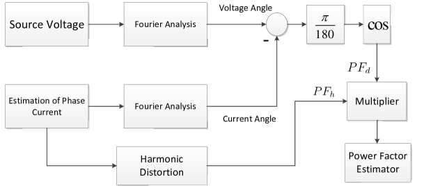
The structure of estimation for the single-phase power factor in MATLAB/SIMULINK is shown in Fig. 4, which includes two important modules: Fourier analysis and Harmonic analysis. The first module gives the phases of main-frequency input current and source phase voltage respectively. The other module is used to measure the total harmonic distortion of input current.

Figure 4: Structure of single-phase power factor calculation

5 SIMULATION RESULTS

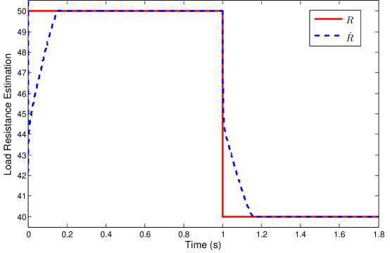
Simulation results are carried out on the proposed three phase AC/DC boost power converter, the parameters used in simulation are shown in Table 5. Load resistance and frequency are varied to test controller’s ability to handle with varying conditions at time $\displaystyle 1.0s$ and $\displaystyle 1.5s$ respectively.

Parameters Used For Simulation. $\displaystyle r$ 0.02 $\displaystyle\Omega$ $\displaystyle C$ 100 $\displaystyle u$F $\displaystyle L$ $\displaystyle 2$ mH $\displaystyle w$ $\displaystyle 150\pi\stackrel{{\scriptstyle t=1.5s}}{{\longrightarrow}}300\pi$ rad/s $\displaystyle R$ $\displaystyle 50\stackrel{{\scriptstyle t=1.0s}}{{\longrightarrow}}40$ $\displaystyle\Omega$ $\displaystyle E$ 150 V $\displaystyle{U_{0}}^{*}$ 650 V $\displaystyle U_{0}(0)$ 5 V

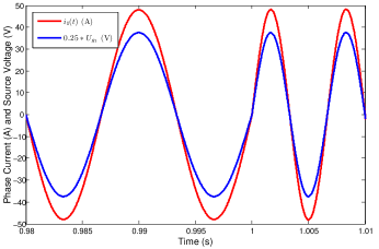
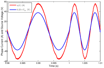
The simulation results of the proposed observer-based ST SMC compared with linear PI regulator (Silva, 1999) are shown in Figs 5-8. Input phase current along with the corresponding source voltage are shown in Fig. 5. From Fig. 5(a) and Fig. 5(b), both of the controller make no phase shift between the input current and corresponding source voltage, however the PI Control results in higher harmonics compared to the ST SMC.

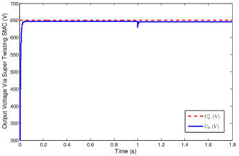
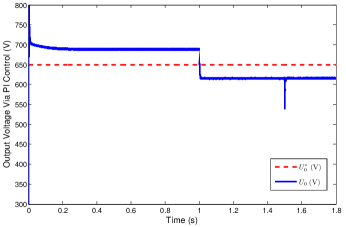
Fig. 6 shows the output voltage performance of the AC/DC converter. From Fig. 6(a) and Fig. 6(b), it is seen that the proposed observer-based ST SMC is able to regulate the output voltage to the desired level under the condition of load variation. A good estimate for the load resistance is shown in Fig. 7. However, the PI Control results in higher fluctuation around some DC level, and higher voltage overshoot compared with the ST SMC. It should be noted that the PI control is not able to demonstrate its robustness with respect to load variation, due to the fact that the gains $\displaystyle k_{p},k_{i}$ of the PI control depend on the load resistance $\displaystyle R_{L}$ (Silva, 1999).

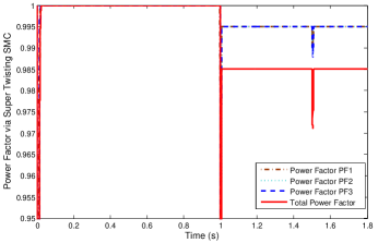
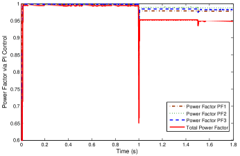
Fig. 8 shows the separate power factor value of each phase and their product as a combined characteristic of the AC/DC converter. From Fig. 8(a) and Fig. 8(b), it is shown that the power factor value are more that 97% in case of observer-based ST SMC, while the PI Control results in less value and more oscillations compared to the ST SMC. The proposed observer-based ST SMC is proven to be able to produce a power factor value that was always more than 97%, and less sensitive to the changing conditions.

6 CONCLUSIONS

An observer-based ST SMC is proposed in this paper for the AC/DC boost converters. The use of observer reduces the number of current sensors, decreases the system cost, volume and provides robustness to the change of operational condition (e.g. in load resistance $\displaystyle R_{L}$ and frequency of the source voltage $\displaystyle\omega$). The proposed observer-based ST SMC maintains the power factor close to unity. A strong Lyapunov function is introduced to prove the stability of the observer and controller as a whole system. Simulation results show that the observer-based controller performs better, compared to conventional PI control, with less overshoot and less sensitivity to disturbance and parametric uncertainty.

(a) The case of observer-based ST SMC

(b) The case of PI Control

Figure 5: Phase current and source voltage ($\displaystyle\times 0.25$)

(a) The case of observer-based ST SMC

(b) The case of PI Control

Figure 6: Output Voltage Performance

Figure 7: Load Resistance Estimation Via Super-Twisting Observer

(a) The case of super-twisting SMC

(b) The case of PI Control

Figure 8: Power factor of the AC/DC converter

References

- Allag et al. (2007) Allag, A., Hammoudi, M., Mimoune, S., Ayad, M., Becherif, M., and Miraoui, A. (2007), “Tracking Control Via Adaptive Backstepping Approach for a Three Phase PWM AC-DC Converter,” in IEEE International Symposium on Industrial Electronics, ISIE, pp. 371–376.
- Amjadi and Williamson (2010) Amjadi, Z., and Williamson, S. (2010), “Power Electronics Based Solutions for Plug-In Hybrid Electric Vehicle Energy Storage and Management Systems,” IEEE Transactions on Industrial Electronics, 57, 608–616.
- Andersen et al. (1999) Andersen, B., Holmgaard, T., Nielsen, J., and Blasbjerg, F. (1999), “Active Three-phase Rectifier with only One Current Sensor in the DC-link,” in Proceedings of the IEEE International Conference on Power Electronics and Drive Systems, Vol. 1, pp. 69–74.
- Besançon (2007) Besançon, G., Nonlinear observers and applications, Vol. 363, Springer Verlag (2007).
- Bose (2002) Bose, B.K., Modern Power Electronics and AC Drives, Prentice Hall (2002).
- Camara et al. (2010) Camara, M., Gualous, H., Gustin, F., Berthon, A., and Dakyo, B. (2010), “DC/DC Converter Design for Supercapacitor and Battery Power Management in Hybrid Vehicle Applications-Polynomial Control Strategy,” IEEE Transactions on Industrial Electronics, 57, 587–597.
- Cao and Emadi (2009) Cao, J., and Emadi, A. (2009), “A New Battery/Ultra-Capacitor Hybrid Energy Storage System for Electric, Hybrid and Plug-In Hybrid Electric Vehicles,” in IEEE Vehicle Power and Propulsion Conference, VPPC’09, pp. 941–946.
- Cecati et al. (2005) Cecati, C., Dell’Aquila, A., Lecci, A., and Liserre, M. (2005), “Implementation Issues of a Fuzzy-Logic-Based Three-Phase Active Rectifier Employing Only Voltage Sensors,” IEEE Transactions on Industrial Electronics, 52, 378–385.
- Dixon and Ooi (1988) Dixon, J., and Ooi, B.T. (1988), “Indirect Current Control of a Unity Power Factor Sinusoidal Current Boost Type Three-Phase Rectifier,” IEEE Transactions on Industrial Electronics, 35, 508–515.
- Edwards and Spurgeon (1998) Edwards, C., and Spurgeon, S., Sliding Mode Control: Theory and Applications, Taylor & Francis (1998).
- Egan et al. (2007) Egan, M., O’Sullivan, D., Hayes, J., Willers, M., and Henze, C. (2007), “Power Factor Corrected Single Stage Inductive Charger for Electric Vehicle Batteries,” IEEE Transactions on Industrial Electronics, 54, 1217–1226.
- Emadi et al. (2008) Emadi, A., Lee, Y.J., and Rajashekara, K. (2008), “Power Electronics and Motor Drives in Electric, Hybrid Electric, and Plug-In Hybrid Electric Vehicles,” IEEE Transactions on Industrial Electronics, 55, 2237–2245.
- Escobar et al. (2001) Escobar, G., Chevreau, D., Ortega, R., and Mendes, E. (2001), “An Adaptive Passivity-Based Controller for a Unity Power Factor Rectifier,” IEEE Transactions on Control Systems Technology, 9, 637–644.
- Guerrero et al. (2013) Guerrero, J., Loh, P.C., Lee, T.L., and Chandorkar, M. (2013), “Advanced Control Architectures for Intelligent Microgrids;Part II: Power Quality, Energy Storage, and AC/DC Microgrids,” IEEE Transactions on Industrial Electronics, 60, 1263–1270.
- Hassan K. Khalil (2007) Hassan K. Khalil,, Nonlinear systems, Vol. 3, Prentice hall New Jersey (2007).
- Hayes et al. (1999) Hayes, J., Egan, M., Murphy, J., Schulz, S., and Hall, J. (1999), “Wide-Load-Range Resonant Converter Supplying the SAE J-1773 Electric Vehicle Inductive Charging Interface,” IEEE Transactions on Industry Applications, 35, 884–895.
- Hermann and Krener (1977) Hermann, R., and Krener, A. (1977), “Nonlinear Controllability and Observability,” IEEE Transactions on Automatic Control, 22, 728–740.
- Hornik and Zhong (2013) Hornik, T., and Zhong, Q.C. (2013), “Parallel PI Voltage– Current Controller for the Neutral Point of a Three-Phase Inverter,” IEEE Transactions on Industrial Electronics, 60, 1335–1343.
- Houari et al. (2012) Houari, A., Renaudineau, H., Martin, J., Pierfederici, S., and Meibody-Tabar, F. (2012), “Flatness-Based Control of Three-Phase Inverter With Output Filter,” IEEE Transactions on Industrial Electronics, 59, 2890–2897.
- Kömürcügil and Kükrer (1998) Kömürcügil, H., and Kükrer, O. (1998), “Lyapunov-Based Control for Three-Phase PWM AC/DC Voltage-Source Converters,” IEEE Transactions on Power Electronics, 13, 801–813.
- Kuperman et al. (2012) Kuperman, A., Levy, U., Goren, J., Zafransky, A., and Savernin, A. (2012), “Battery Charger for Electric Vehicle Traction Battery Switch Station,” IEEE Transactions on Industrial Electronics, p. 1.
- Lee et al. (2000) Lee, D.C., Lee, G.M., and Lee, K.D. (2000), “DC-bus Voltage Control of Three-Phase AC/DC PWM Converters Using Feedback Linearization,” IEEE Transactions on Industry Applications, 36, 826–833.
- Lee and Lim (2002) Lee, D.C., and Lim, D.S. (2002), “AC Voltage and Current Sensorless Control of Three-Phase PWM Rectifiers,” IEEE Transactions on Power Electronics, 17, 883–890.
- Lee (2003) Lee, T.S. (2003), “Input-Output Linearization and Zero-Dynamics Control of Three-Phase AC/DC Voltage-Source Converters,” IEEE Transactions on Power Electronics, 18, 11–22.
- Lee et al. (2001) Lee, W.C., Lee, T.K., and Hyun, D.S. (2001), “Comparison of Single-Sensor Current Control in the DC Link for Three-Phase Voltage-Source PWM Converters,” IEEE Transactions on Industrial Electronics, 48, 491–505.
- Lee et al. (2009) Lee, Y.J., Khaligh, A., and Emadi, A. (2009), “Advanced Integrated Bidirectional AC/DC and DC/DC Converter for Plug-In Hybrid Electric Vehicles,” IEEE Transactions on Vehicular Technology, 58, 3970–3980.
- Levant (1993) Levant, A. (1993), “Sliding Order and Sliding Accuracy in Sliding Mode Control,” International Journal of Control, 58, 1247–1263.
- Levant (1998) Levant, A. (1998), “Robust Exact Differentiation via Sliding Mode Technique,” Automatica, 34, 379–384.
- Levant (2007) Levant, A. (2007), “Principles of 2-Sliding Mode Design,” Automatica, 43, 576–586.
- Liu et al. (2013) Liu, X., Loh, P.C., Wang, P., and Blaabjerg, F. (2013), “A Direct Power Conversion Topology for Grid Integrations of Hybrid AC/DC Resources,” IEEE Transactions on Industrial Electronics, p. 1.
- Pahlevaninezhad et al. (2012b) Pahlevaninezhad, M., Das, P., Drobnik, J., Jain, P., and Bakhshai, A. (2012b), “A New Control Approach Based on the Differential Flatness Theory for an AC/DC Converter Used in Electric Vehicles,” IEEE Transactions on Power Electronics, 27, 2085–2103.
- Pahlevaninezhad et al. (2012a) Pahlevaninezhad, M., Das, P., Drobnik, J., Moschopoulos, G., Jain, P., and Bakhshai, A. (2012a), “A Nonlinear Optimal Control Approach Based on the Control-Lyapunov Function for an AC/DC Converter Used in Electric Vehicles,” IEEE Transactions on Industrial Informatics, 8, 596–614.
- Pan and Chen (1993) Pan, C., and Chen, T. (1993), “Modelling and Analysis of a Three Phase PWM AC-DC Convertor Without Current Sensor,” IEE Proceedings B, Electric Power Applications, 140, 201–208.
- Pu et al. (2012) Pu, X., Nguyen, T., Lee, D., Lee, K., and Kim, J. (2012), “Fault Diagnosis of DC-Link Capacitors in Three-Phase AC/DC PWM Converters by Online Estimation of Equivalent Series Resistance,” IEEE Transactions on Industrial Electronics, p. 1.
- Sabanovic et al. (2004) Sabanovic, A., Fridman, L., and Spurgeon, S.K., Variable Structure Systems: From Principles to Implementation, IET (2004).
- Sarinana et al. (2000) Sarinana, A., Bacha, S., and Bornard, G. (2000), “On Nonlinear Observers Applied to Three-Phase Voltage Source Converters,” in 31st IEEE Annual Power Electronics Specialists Conference, Vol. 3, pp. 1419–1424.
- Shtessel et al. (2008) Shtessel, Y., Baev, S., and Biglari, H. (2008), “Unity Power Factor Control in Three-Phase AC/DC Boost Converter Using Sliding Modes,” IEEE Transactions on Industrial Electronics, 55, 3874–3882.
- Silva (1997) Silva, J. (1997), “Sliding Mode Control of Voltage Sourced Boost-Type Reversible Rectifiers,” in Proceedings of the IEEE International Symposium on Industrial Electronics, Vol. 2, pp. 329–334.
- Silva (1999) Silva, J. (1999), “Sliding Mode Control of Boost-Type Unity-Power-Factor PWM Rectifiers,” IEEE Transactions on Industrial Electronics, 46, 594–603.
- Sira-Ramirez et al. (1996) Sira-Ramirez, H., Escobar, G., and Ortega, R. (1996), “On Passivity-Based Sliding Mode Control of Switched DC-to-DC Power Converters,” in Proceedings of the 35th IEEE Decision and Control, Vol. 3, pp. 2525–2526.
- Tan et al. (2007) Tan, S.C., Lai, Y., Tse, C., Martinez-Salamero, L., and Wu, C.K. (2007), “A Fast-Response Sliding-Mode Controller for Boost-Type Converters With a Wide Range of Operating Conditions,” IEEE Transactions on Industrial Electronics, 54, 3276–3286.
- Thounthong (2012) Thounthong, P. (2012), “Control of a Three-Level Boost Converter Based on a Differential Flatness Approach for Fuel Cell Vehicle Applications,” IEEE Transactions on Vehicular Technology, 61, 1467–1472.
- Vadim Utkin, Jurgen Guldner, Jingxin Shi (2009) Vadim Utkin, Jurgen Guldner, Jingxin Shi,, Sliding Mode Control in Electro-Mechanical Systems, CRC Press, Taylor and Francis Group (2009).
- Wirasingha and Emadi (2011) Wirasingha, S., and Emadi, A. (2011), “Classification and Review of Control Strategies for Plug-In Hybrid Electric Vehicles,” IEEE Transactions on Vehicular Technology, 60, 111–122.
- Zhong and Hornik (2013) Zhong, Q.C., and Hornik, T. (2013), “Cascaded Current-Voltage Control to Improve the Power Quality for a Grid-Connected Inverter With a Local Load,” IEEE Transactions on Industrial Electronics, 60, 1344–1355.