Adaptive-Gain Second-Order Sliding Mode Observer Design for Switching Power Converters

Abstract

In this paper, a novel adaptive-gain, Second Order Sliding Mode (SOSM) observer for multi-cell converters is designed by considering it as a type of hybrid system. The objective is to reduce the number of voltage sensors by estimating the capacitor voltages from only measurements of the load current. The proposed observer is proven to be robust in the presence of perturbations with unknown boundaries. However, the states of the system are only partially observable based on the observability matrix rank condition. Because its observability depends upon the switching control signals, a recent concept known as $\displaystyle Z(T_{N})$-observability, which can be used to analyze the observability of hybrid systems, is used to address the switching behavior. Under certain conditions of the switching sequences, the voltage across each capacitor becomes observable. Simulation results and comparisons with a Luenberger switched observer demonstrate the effectiveness and the robustness of the proposed observer with respect to output measurement noise and system uncertainties (load variations).

1 INTRODUCTION

In recent years, industrial applications requiring high power levels have used medium-voltage semiconductors (Meynard & Foch, 1992; Rodriguez et al., 2002; Rech & Pinheiro, 2007; Gerry et al., 2003). Because of the efficiency requirements, the power of the converter is generally increased by boosting the voltage. However, medium-voltage switching devices are not available. Even if they did exist, the volume and the cost of such devices would be substantial (Gateau et al., 2002). In this sense, the topology of multi-level converters, which have been studied during the last decade, becomes attractive for high voltage applications (Meynard & Foch, 1992). From a practical point of view, the series of a multi-cell chopper designed by the LEEI (Toulouse, France) (Bensaid & Fadel, 2001a), leads to a safe series association of components working in a switching mode. This structure offers the possibility of reducing the voltage constraints evenly among each cell in a series. These lower-voltage switches result in lower conduction losses and higher switching frequencies. Moreover, it is possible to improve the output waveforms using this structure (Bensaid & Fadel, 2001b; Gateau et al., 2002; Bensaid & Fadel, 2002). These flying capacitors have to be balanced to guarantee the desired voltage values at the output, which ensures that the maximum benefit from the multi-cell structure is obtained (Meynard et al., 1997). These properties are lost if the capacitor voltage drifts far from the desired value (Bejarano et al., 2010). Therefore, a suitable control of the switches is required to generate the desired values of the capacitor voltages. The control of switches allows the current harmonics at the cutting frequency to be canceled and the ripple of the chopped voltage to be reduced (Djemaï et al., 2011; Defoort et al., 2011).

Several control methods have been proposed for multi-cell converters, such as nonlinear control based on input-output linearization (Gateau et al., 2002), predictive control (Defaÿ et al., 2008), hybrid control (Bâja et al., 2007), model predictive control (Defaÿ et al., 2008; Lezana et al., 2009) and sliding mode control (Djemaï et al., 2011; L. Amet, M. Ghanes, J.P. Barbot, 2011; Meradi et al., 2013). However, most of these techniques require measurements of the voltages of the capacitors to design the controller. That is, extra voltage sensors are necessary, which increases the cost and the complexity of the system. Hence, the estimation of the capacitor voltages using an observer has attracted great interest (Besançon, 2007).

It should be noted that the states of the multi-cell system are only partially observable because the observability matrix never has full rank (Besançon, 2007). Hence, the observability matrix rank condition cannot be employed in an observability analysis of a hybrid system such as the one considered here (Vidal et al., 2003; Babaali & Pappas, 2005). A recent concept, $\displaystyle Z(T_{N})$-observability (Kang et al., 2009), can be used to analyze the observability of a switched hybrid system and is applied in this work because the observability of the converter depends upon the switching control signals. Various observers have been designed for the multi-cell converters based on concepts such as homogeneous finite-time observers (Defoort et al., 2011), super-twisting sliding mode observers (Bejarano et al., 2010; M. Ghanes, F. Bejarano and J.P. Barbot, 2009) and adaptive observer (Bejarano et al., 2010). The concept of observability presented in Kang et al. (2009) gives the condition under which there exists a hybrid time trajectory that makes the system observable. Using this concept, estimates of the capacitor voltages can be obtained from the measurements of the load current and the source voltage by taking advantage of the appropriate hybrid time trajectories.

In this paper, an observability analysis based on the results of Kang et al. (2009) is performed for the multi-cell converter assuming measurements of the load current and the source voltage under certain conditions of the switching input sequences. Then, a novel adaptive-gain SOSM observer for multi-cell converters is introduced that takes into account certain perturbations (load variations) in which the boundaries of their first time derivatives are unknown. The proposed adaptive-gain SOSM algorithm combines the nonlinear term of the super-twisting algorithm and a linear term, the so-called SOSML algorithm (Moreno & Osorio, 2008). The behavior of the SOSM algorithm near the origin is significantly improved compared with the linear case. Conversely, the additional linear term improves the behavior of the SOSM algorithm when the states are far from the origin. Therefore, the SOSML algorithm inherits the best properties of both the linear and the nonlinear terms. An adaptive law of the gains of the SOSML algorithm is derived via the so-called ”time scaling” approach (Respondek et al., 2004). The output observation error and its first time derivative converge to zero in finite time with the proposed SOSML observer such that the equivalent output-error injection can be obtained directly. Finally, the resulting reduced-order system is proven to be exponentially stable. That is, the observer error for the capacitor voltages, which are considered as the states of the observer system, converge to zero exponentially. The main advantages of the proposed adaptive-gain SOSML are that only one parameter has to be tuned and there are no a-priori requirements on the perturbation bounds.

This paper is organized as follows. In Section $\displaystyle\mathrm{II}$, a model of the multi-cell converter and its characteristics are presented. In Section $\displaystyle\mathrm{III}$, the observability of the multi-cell converter is studied with the concept of $\displaystyle Z(T_{N})$-observability. Section $\displaystyle\mathrm{IV}$ discusses the design of the proposed adaptive-gain SOSML observer for estimating the capacitor voltages. Section $\displaystyle\mathrm{V}$ gives simulation results including a comparison with a Luenberger switched observer with disturbances.

2 MODELING OF the MULTI-CELL CONVERTER

The structure of a multi-cell converter is based on the combination of a certain number of cells. Each cell consists of an energy storage element and commutators (Gateau et al., 2002). The main advantage of this structure is that the spectral quality of the output signal is improved by a high switching frequency between the intermediate voltage levels (McGrath & Holmes, 2007). An instantaneous model that was presented in Gateau et al. (2002) and describes fully the hybrid behavior of the multi-cell converter is used here.

Figure 1 depicts the topology of a converter with $\displaystyle p$ independent commutation cells that is connected to an inductive load. The current $\displaystyle I$ flows from the source $\displaystyle E$ to the output through the various converter switches. The converter thus has a hybrid behavior because of the presence of both discrete variables (the switching logic) and continuous variables (the currents and the voltages).

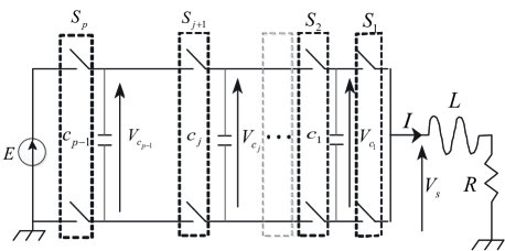
Figure 1: Multicell converter on RL load

Through circuit analysis, the dynamics of the p-cell converter were obtained as the following differential equations:

$$\left\{\begin{split}\dot{I}&=-\frac{R}{L}I+\frac{E}{L}S_{p}-\sum_{j=1}^{p-1}\frac{V_{c_{j}}}{L}(S_{j+1}-S_{j}),\\ \dot{V}_{c_{1}}&=\frac{I}{c_{1}}(S_{2}-S_{1}),\\ &\vdots\\ \dot{V}_{c_{p-1}}&=\frac{I}{c_{p}}(S_{p}-S_{p-1}).\end{split}\right.$$ (1)

where $\displaystyle I$ is the load current, $\displaystyle c_{j}$ is the $\displaystyle j^{th}$ capacitor, $\displaystyle V_{c_{j}}$ is the voltage of the $\displaystyle j^{th}$ capacitor and $\displaystyle E$ is the voltage of the source. Each commutation cell is controlled by the binary input signal $\displaystyle S_{j}\in\{0,1\}$, where $\displaystyle S_{j}=1$ indicates that the upper switch of the $\displaystyle j$th cell is on and the lower switch is off and $\displaystyle S_{j}=0$ indicates that the upper switch is off and the lower switch is on. The discrete inputs are defined as follows:

$$\left\{\begin{split}u_{j}=&S_{j+1}-S_{j},\quad j=1,\ldots,p-1\\ u_{p}=&S_{p}.\end{split}\right.$$ (2)

With equation (2), the system (1) can be represented as follows:

$$\left\{\begin{split}&\dot{I}=-\frac{R}{L}I+\frac{E}{L}u_{p}-\sum_{j=1}^{p-1}\frac{V_{c_{j}}}{L}u_{j},\\ &\dot{V}_{c_{1}}=\frac{I}{c_{1}}u_{1},\\ &\vdots\\ &\dot{V}_{c_{p-1}}=\frac{I}{c_{p-1}}u_{p-1},\\ &y=I.\end{split}\right.$$ (3)

Assuming that only the load current $\displaystyle I$ can be measured, it is easy to represent the system (3) as a hybrid (switched affine) system:

$$\left\{\begin{split}\dot{x}=&f(x,u)=A(u)x+B(u),\\ y=&h(x,u)=Cx.\end{split}\right.$$ (4)

where $\displaystyle x=\begin{bmatrix}I&V_{c_{1}}&\cdots&V_{c_{p-1}}\end{bmatrix}^{T}$ is the continuous state vector,
$\displaystyle u=\begin{bmatrix}u_{1}&u_{2}&\cdots&u_{p}\end{bmatrix}^{T}$ is the switching control signal vector which takes only discrete values and the matrices $\displaystyle A(u)$, $\displaystyle B(u)$, $\displaystyle C$ are defined as:

$$\begin{split}A(u)&=\begin{bmatrix}-\frac{R}{L}&-\frac{u_{1}}{L}&\cdots&-\frac{u_{p-1}}{L}\\ \frac{u_{1}}{c_{1}}&0&\cdots&0\\ \vdots&\vdots&\ddots&\vdots\\ \frac{u_{p-1}}{c_{p-1}}&0&\cdots&0\end{bmatrix},\\ B(u)&=\begin{bmatrix}\frac{E}{L}u_{p}&0&\cdots&0\end{bmatrix}^{T},\\ C&=\begin{bmatrix}1&0&\cdots&0\end{bmatrix}.\end{split}$$ (5)

The main objective of this paper is to design an observer based on the instantaneous model (3) that is able to estimate the capacitor voltages using only the measurement of the load current and the associated switching control input (which is assumed to be known).

3 HYBRID OBSERVABILITY ANALYSIS

From the instantaneous model of the system (4) with $\displaystyle p\geq 3$, it can be noted that there are several switching modes that make the system unobservable. For instance, if $\displaystyle u_{1}=u_{2}=\cdots=u_{p-1}=0$, the voltages $\displaystyle V_{c_{j}}(j={1,\ldots,p-1})$ become completely unobservable. These switching modes are not affected by the capacitor voltages. Fortunately, these cases are ones in which the $\displaystyle p$-cells are not switching and will not occur for all control sequences; otherwise, there is no interest in the physical sense.

The observability analysis of the system (4) is based on the measurement of the load current $\displaystyle I$ and the knowledge of the control input sequence $\displaystyle u$. The so-called observability matrix (Besançon, 2007) is defined as

$$\begin{split}\mathcal{O}_{p\times p}&=\begin{bmatrix}C\\ CA\\ CA^{2}\\ \vdots\\ CA^{p-1}\end{bmatrix}=\begin{bmatrix}1&0&\cdots&0\\ -\frac{R}{L}&-\frac{u_{1}}{L}&\cdots&-\frac{u_{p-1}}{L}\\ (\frac{R}{L})^{2}-\sum^{p-1}_{i=1}\frac{u^{2}_{i}}{Lc_{i}}&\frac{Ru_{1}}{L^{2}}&\cdots&\frac{Ru_{p-1}}{L^{2}}\\ \vdots&\vdots&\vdots&\vdots\\ \end{bmatrix}.\end{split}$$ (6)

With simple computations, it can be shown that

$$\begin{split}rank(\mathcal{O})&=2<p.\end{split}$$ (7)

It follows that the continuous states are not observable using only the load current because the observability matrix (7) is not full rank.

Because of the switching sequences of the system (4), the observability is strongly linked to the hybrid behavior. Therefore, the recently developed concept of $\displaystyle Z(T_{N})$-observability (Kang et al., 2009) is applied to analyze the observability of the hybrid system (4). It is important to note the following definitions.

Definition 1.

Kang et al. (2009) A hybrid time trajectory is a finite or infinite sequence of intervals $\displaystyle T_{N}={\Gamma}^{N}_{i=0}$ such that

• $\displaystyle\Gamma_{i}=[t_{i,0},t_{i,1}),for$ $\displaystyle all$ $\displaystyle 0\leq i<N$;

• For all $\displaystyle i<N,$ $\displaystyle t_{i,1}=t_{i+1,0}$;

• $\displaystyle t_{0,0}=t_{ini}$ $\displaystyle and$ $\displaystyle t_{N,1}=t_{end}$.

Moreover, $\displaystyle\langle T_{N}\rangle$ is defined as the ordered list of inputs $\displaystyle u$ associated with $\displaystyle T_{N}$, $\displaystyle{u^{i}}_{i=0,N}$, where $\displaystyle u^{i}$ is the value of $\displaystyle u$ on the interval $\displaystyle\Gamma_{i}$.

Definition 2.

(Kang et al., 2009) The function $\displaystyle z=Z(t,x)$ is said to be $\displaystyle Z-$observable with respect to the hybrid time trajectory $\displaystyle T_{N}$ and $\displaystyle\langle T_{N}\rangle$ if for any two trajectories $\displaystyle(t,x,u)$ and $\displaystyle(t,x^{\prime},u^{\prime})$ defined in $\displaystyle[t_{ini},t_{end}]$, the equality $\displaystyle h(x,u)=h(x^{\prime},u^{\prime})$ implies that $\displaystyle Z(t,x)=Z(t,x^{\prime})$.

Lemma 1.

(Kang et al., 2009) Consider the system (4) and a fixed hybrid time trajectory $\displaystyle T_{N}$ and $\displaystyle\langle T_{N}\rangle$. Suppose that $\displaystyle z=Z(t,x)$ is always continuous under any admissible control input. If there exists a sequence of projections $\displaystyle{P_{i}},$ $\displaystyle i=0,1,\cdots,N$, such that

• For all $\displaystyle i<N$, $\displaystyle P_{i}Z(t,x)$ is $\displaystyle Z-$observable for $\displaystyle t\in\Gamma_{i}$;

• Rank$\displaystyle([P^{T}_{0},\cdots,P^{T}_{N}])=dim(z)$;

• $\displaystyle\frac{d\bar{P}_{i}Z(t,x)}{dt}=0$, for $\displaystyle t\in\Gamma_{i}$, where $\displaystyle\bar{P}$ is the complement of $\displaystyle P$(projecting $\displaystyle z$ to the variables eliminated by $\displaystyle P$),

then, $\displaystyle z=Z(t,x)$ is $\displaystyle Z-$observable with respect to the hybrid time trajectory $\displaystyle T_{N}$ and $\displaystyle\langle T_{N}\rangle$.

Proof.

The proof of the Lemma 1 can be found in Kang et al. (2009). ∎

Remark 1.

In Lemma 1, the third condition requires that the components of $\displaystyle Z$ that are not observable in $\displaystyle\Gamma_{i}$ must remain constant within this time interval. The hybrid time trajectory $\displaystyle T_{N}$ and $\displaystyle\langle T_{N}\rangle$ influences the observability property in a way similar to an input.

Table 1 presents the eight possible configurations for a three-cell converter. The application of Lemma 1 to the three-cell converter is as follows. We take $\displaystyle Z(t,x)=\begin{bmatrix}x_{2}&x_{3}\end{bmatrix}^{T}=\begin{bmatrix}V_{c_{1}}&V_{c_{2}}\end{bmatrix}^{T}$. For the discrete switching conditions $\displaystyle[0,0,0]$ and $\displaystyle[1,1,1]$, it can be verified that $\displaystyle Z(t,x)$ is not $\displaystyle Z(T_{N})$-observable. Fortunately, from (1) the dynamics of $\displaystyle V_{c_{1}}$ and $\displaystyle V_{c_{2}}$ are zero, which means that these states remain constant during these time intervals. Next, assume that a trajectory of the system has the status $\displaystyle[1,0,0]$ and $\displaystyle[1,1,0]$ during time intervals $\displaystyle\Gamma_{1}$ and $\displaystyle\Gamma_{2}$, respectively. Let us define $\displaystyle P_{1}=\begin{bmatrix}1&0\end{bmatrix}$ and $\displaystyle P_{2}=\begin{bmatrix}0&1\end{bmatrix}$. We have $\displaystyle\bar{P}_{1}Z=x_{3}=V_{c_{2}}$, $\displaystyle\frac{d\bar{P}_{1}Z}{dt}=\frac{dV_{c_{2}}}{dt}=0$, $\displaystyle\bar{P}_{2}Z=x_{2}=V_{c_{1}}$, $\displaystyle\frac{d\bar{P}_{2}Z}{dt}=\frac{dV_{c_{1}}}{dt}=0$ and $\displaystyle rank\begin{bmatrix}P_{1}\\ P_{2}\end{bmatrix}=2$. All the assumptions in Lemma 1 are satisfied; therefore, $\displaystyle Z(t,x)=\begin{bmatrix}V_{c_{1}}&V_{c_{2}}\end{bmatrix}^{T}$ is $\displaystyle Z(T_{N})$-observable.

Table 1: Switching modes and capacitor voltages for a three-cell converter

Mode : $\displaystyle[S_{1},S_{2},S_{3}]$	$\displaystyle V_{c_{1}}$	$\displaystyle V_{c_{2}}$	$\displaystyle u_{1}$	$\displaystyle u_{2}$	Observable States
0 : [0,0,0]	$\displaystyle\rightsquigarrow$	$\displaystyle\rightsquigarrow$	0	0	$\displaystyle I$
1 : [0,0,1]	$\displaystyle\rightsquigarrow$	$\displaystyle\nearrow$	0	1	$\displaystyle I,V_{c_{2}}$
2 : [0,1,0]	$\displaystyle\nearrow$	$\displaystyle\searrow$	1	-1	$\displaystyle I,V_{c_{1}},V_{c_{2}}$
3 : [0,1,1]	$\displaystyle\nearrow$	$\displaystyle\rightsquigarrow$	1	0	$\displaystyle I,V_{c_{1}}$
4 : [1,0,0]	$\displaystyle\searrow$	$\displaystyle\rightsquigarrow$	-1	0	$\displaystyle I,V_{c_{1}}$
5 : [1,0,1]	$\displaystyle\searrow$	$\displaystyle\nearrow$	-1	1	$\displaystyle I,V_{c_{1}},V_{c_{2}}$
6 : [1,1,0]	$\displaystyle\rightsquigarrow$	$\displaystyle\searrow$	0	-1	$\displaystyle I,V_{c_{2}}$
7 : [1,1,1]	$\displaystyle\rightsquigarrow$	$\displaystyle\rightsquigarrow$	0	0	$\displaystyle I$

The symbols in Table 1 are defined as follows: $\displaystyle\rightsquigarrow$ indicates a constant value, $\displaystyle\nearrow$ indicates increasing and $\displaystyle\searrow$ indicates decreasing.

In the next section, an adaptive-gain SOSML observer will be presented for the converter system (3).

4 ADAPTIVE-GAIN SOSML OBSERVER DESIGN

As discussed in Gateau et al. (2002), active control of the multi-cell converter requires the knowledge of the capacitor voltages. Usually, voltage sensors are used to measure the capacitor voltages. However, the extra sensors increase the cost, the complexity and the size, especially in high-voltage applications. Moreover, any sensors will introduce the measurement noise which will be directly transposed to the estimated value. Therefore, the design of a state observer using only the measurement of load current and the associated switching inputs is desirable.

In this section, an adaptive-gain SOSML observer for the three-cell converter ($\displaystyle p=3$) is presented that is robust to perturbations (load variations) for which the boundaries of the first time derivative are unknown. A novel adaptive law for the gains of the SOSML algorithm with only one tuning parameter is designed via the so-called ”time scaling” approach (Respondek et al., 2004). The proposed approach does not require the a-priori knowledge of the perturbation bounds.

Defining $\displaystyle e_{1}=I-\hat{I}$, the system (3) is rewritten to include the perturbation $\displaystyle\tilde{f}(e_{1})$, i.e., the load resistance uncertainty (Defoort et al., 2011),

$$\left\{\begin{split}&\dot{I}=-\frac{R}{L}I+\frac{E}{L}u_{3}-\frac{V_{c_{1}}}{L}u_{1}-\frac{V_{c_{2}}}{L}u_{2}+\tilde{f}(e_{1}),\\ &\dot{V}_{c_{1}}=\frac{u_{1}}{c_{1}}I,\\ &\dot{V}_{c_{2}}=\frac{u_{2}}{c_{2}}I.\end{split}\right.$$ (8)

The proposed observer is formulated as

$$\left\{\begin{split}&\dot{\hat{I}}=-\frac{R}{L}I+\frac{E}{L}u_{3}-\frac{\hat{V}_{c_{1}}}{L}u_{1}-\frac{\hat{V}_{c_{2}}}{L}u_{2}+\mu(e_{1}),\\ &\dot{\hat{V}}_{c_{1}}=\frac{u_{1}}{c_{1}}I+k_{1}\mu(e_{1}),\\ &\dot{\hat{V}}_{c_{2}}=\frac{u_{2}}{c_{2}}I+k_{2}\mu(e_{1}).\end{split}\right.$$ (9)

where $\displaystyle\mu(\cdot)$ is the SOSML algorithm (Moreno & Osorio, 2008),

$$\mu(e_{1})=\lambda(t)|e_{1}|^{\frac{1}{2}}sign(e_{1})+\alpha(t)\int^{t}_{0}sign(e_{1})d\tau+k_{\lambda}(t)e_{1}+k_{\alpha}(t)\int^{t}_{0}e_{1}d\tau,$$ (10)

and the adaptive gains $\displaystyle\lambda(t),\alpha(t),k_{\lambda}(t),k_{\alpha}(t)$ and the design parameters $\displaystyle k_{1}$ and $\displaystyle k_{2}$ are to be defined.

Define the observation errors as

$$\left\{\begin{split}e_{2}=&V_{c_{1}}-\hat{V}_{c_{1}},\\ e_{3}=&V_{c_{2}}-\hat{V}_{c_{2}}.\end{split}\right.$$ (11)

Equations (8) and (9) yield the observation error dynamics as:

$$\displaystyle\dot{e}_{1} \displaystyle= \displaystyle-\mu(e_{1})-\frac{u_{1}}{L}e_{2}-\frac{u_{2}}{L}e_{3}+\tilde{f}(e_{1}),$$ (12)

$$\displaystyle\dot{e}_{2} \displaystyle= \displaystyle-k_{1}\mu(e_{1}),$$ (13)

$$\displaystyle\dot{e}_{3} \displaystyle= \displaystyle-k_{2}\mu(e_{1}).$$ (14)

In this paper, the adaptive gains $\displaystyle\lambda(t),\alpha(t),k_{\lambda}(t)$ and $\displaystyle k_{\alpha}(t)$ are formulated as

$$\left\{\begin{split}\lambda(t)&=\lambda_{0}\sqrt{l(t)},\\ \alpha(t)&=\alpha_{0}l(t),\\ k_{\lambda}(t)&=k_{\lambda_{0}}l(t),\\ k_{\alpha}(t)&=k_{\alpha_{0}}l^{2}(t).\end{split}\right.$$ (15)

where $\displaystyle\lambda_{0},\alpha_{0},k_{\lambda_{0}}$ and $\displaystyle k_{\alpha_{0}}$ are positive constants to be defined and $\displaystyle l(t)$ is a positive, time-varying, scalar function.

The adaptive law of the time-varying function $\displaystyle l(t)$ and the design parameters $\displaystyle k_{1}$ and $\displaystyle k_{2}$ are given by:

$$\dot{l}(t)=\begin{cases}k,\quad\quad if\quad|e_{1}|\neq 0\\ 0,\quad\quad else\end{cases}$$ (16)

$$\begin{split}k_{1}=&\begin{cases}-\kappa u_{1},\ \ if\ \ |e_{1}|=0\\ 0.\ \ \quad\quad else\end{cases},\quad k_{2}=\begin{cases}-\kappa u_{2},\ \ if\ \ |e_{1}|=0\\ 0.\ \ \quad\quad else\end{cases}\end{split}$$ (17)

where $\displaystyle k$, the initial value $\displaystyle l(0)$ and $\displaystyle\kappa$ are positive constants.

Assumption 1.

The system (8) and the observer system (9) are bounded input, bounded state (BIBS) because this is a physical system (Perruquetti & Barbot, 2002).

Assumption 2.

There is a $\displaystyle T_{N}$ such that $\displaystyle z=x=\begin{bmatrix}I&V_{c_{1}}&V_{c_{2}}\end{bmatrix}^{T}$ is Z-observable under the condition of Lemma 1 (Defoort et al., 2011).

Theorem 1.

Consider the error system (12) under Assumptions (1) and (2). Assume that the perturbation $\displaystyle\tilde{f}(e_{1})$ satisfies the following condition:

$$\begin{split}\left|\dot{\tilde{f}}(e_{1})\right|\leq\chi_{1},\ \ and\ \ \tilde{f}(0)=0.\end{split}$$ (18)

where $\displaystyle\chi_{1}$ is an unknown positive constant. Then, the trajectories of the error system (12) converge to zero in finite time with the adaptive gains in (15) and (16) satisfying the following condition:

$$4\alpha_{0}k_{\alpha_{0}}>8k^{2}_{\lambda_{0}}\alpha_{0}+9\lambda^{2}_{0}k^{2}_{\lambda_{0}},$$ (19)

Proof.

The system (12) can be rewritten as

$$\left\{\begin{split}\dot{e}_{1}&=-\lambda(t)|e_{1}|^{\frac{1}{2}}sign(e_{1})-k_{\lambda}(t)e_{1}+\varphi_{1},\\ \dot{\varphi}_{1}&=-\alpha(t)sign(e_{1})-k_{\alpha}(t)e_{1}+\varrho_{1}.\end{split}\right.$$ (20)

where $\displaystyle\varrho_{1}=\left(\dot{\tilde{f}}(e_{1})-\frac{u_{1}}{L}\dot{e}_{2}-\frac{u_{2}}{L}\dot{e}_{3}\right)$.

Based on Assumption 1, because the input $\displaystyle u$ is bounded, the state does not go to infinity in finite time. Moreover, if $\displaystyle\hat{I}$ is bounded, all the states of the observer are also bounded for a finite time. Consequently, the observation error $\displaystyle e_{1}$ is also bounded (Perruquetti & Barbot, 2002). It follows from (13, 14) that $\displaystyle\dot{e}_{2}$ and $\displaystyle\dot{e}_{3}$ are bounded and satisfy $\displaystyle|\dot{e}_{2}|\leq\chi_{2}$ and $\displaystyle|\dot{e}_{3}|\leq\chi_{3}$, where $\displaystyle\chi_{2}$ and $\displaystyle\chi_{3}$ are some unknown positive values. From equation (18), it is easy to deduce that $\displaystyle|\varrho_{1}|\leq\chi_{1}+\frac{\chi_{2}}{L}+\frac{\chi_{3}}{L}=F$, where $\displaystyle F$ is an unknown positive value.

A new state vector is introduced to represent the system in (20) in a more convenient form for Lyapunov analysis.

$$\zeta=\begin{bmatrix}\zeta_{1}\\ \zeta_{2}\\ \zeta_{3}\end{bmatrix}=\begin{bmatrix}l^{\frac{1}{2}}(t)|e_{1}|^{\frac{1}{2}}sign(e_{1})\\ l(t)e_{1}\\ \varphi_{1}\end{bmatrix},$$ (21)

Thus, the system in (20) can be rewritten as

$$\begin{split}\dot{\zeta}&=\frac{l(t)}{|\zeta_{1}|}\underbrace{\begin{bmatrix}-\frac{\lambda_{0}}{2}&0&\frac{1}{2}\\ 0&-\lambda_{0}&0\\ -\alpha_{0}&0&0\end{bmatrix}}_{A_{1}}\zeta+l(t)\underbrace{\begin{bmatrix}-\frac{k_{\lambda_{0}}}{2}&0&0\\ 0&-k_{\lambda_{0}}&1\\ 0&-k_{\alpha_{0}}&0\end{bmatrix}}_{A_{2}}\zeta+\begin{bmatrix}\frac{\dot{l}}{2l(t)}\zeta_{1}\\ \frac{\dot{l}}{2l(t)}\zeta_{2}\\ \varrho_{1}\end{bmatrix},\end{split}$$ (22)

Then, the following Lyapunov function candidate is introduced for the system in (22):

$$V(\zeta)=2\alpha_{0}\zeta^{2}_{1}+k_{\alpha_{0}}\zeta^{2}_{2}+\frac{1}{2}\zeta^{2}_{3}+\frac{1}{2}\left(\lambda_{0}\zeta_{1}+k_{\lambda_{0}}\zeta_{2}-\zeta_{3}\right)^{2},$$ (23)

which can be rewritten as a quadratic form

$$V(\zeta)=\zeta^{T}P\zeta,\quad P=\frac{1}{2}\begin{bmatrix}4\alpha_{0}+\lambda^{2}_{0}&\lambda_{0}k_{\lambda_{0}}&-\lambda_{0}\\ \lambda_{0}k_{\lambda_{0}}&k^{2}_{\lambda_{0}}+2k_{\alpha_{0}}&-k_{\lambda_{0}}\\ -\lambda_{0}&-k_{\lambda_{0}}&2\end{bmatrix}.$$ (24)

As (23) is a continuous Lyapunov function, the matrix $\displaystyle P$ is positive definite.

Taking the derivative of (24) along the trajectories of (22),

$$\begin{split}\dot{V}=-\frac{l(t)}{|\zeta_{1}|}\zeta^{T}\Omega_{1}\zeta-l(t)\zeta^{T}\Omega_{2}\zeta+\varrho_{1}q_{1}\zeta+\frac{\dot{l}}{l(t)}q_{2}P\zeta,\end{split}$$ (25)

where $\displaystyle q_{1}=\begin{bmatrix}-\lambda_{0}&-k_{\lambda_{0}}&2\end{bmatrix}$, $\displaystyle q_{2}=\begin{bmatrix}\zeta_{1}&\zeta_{2}&0\end{bmatrix}$, and

$$\begin{split}\Omega_{1}&=\frac{\lambda_{0}}{2}\begin{bmatrix}\lambda^{2}_{0}+2\alpha_{0}&0&-\lambda_{0}\\ 0&2k_{\alpha_{0}}+5k^{2}_{\lambda_{0}}&-3k_{\lambda_{0}}\\ -\lambda_{0}&-3k_{\lambda_{0}}&1\end{bmatrix},\\ \Omega_{2}&=k_{\lambda_{0}}\begin{bmatrix}\alpha_{0}+2\lambda^{2}_{0}&0&0\\ 0&k_{\alpha_{0}}+k^{2}_{\lambda_{0}}&-k_{\lambda_{0}}\\ 0&-k_{\lambda_{0}}&1\end{bmatrix}.\end{split}$$ (26)

it is easy to verify that $\displaystyle\Omega_{1}$ and $\displaystyle\Omega_{2}$ are positive definite matrices under the condition in (19).

Because $\displaystyle\lambda_{min}(P)\|\zeta\|^{2}\leq V\leq\lambda_{max}(P)\|\zeta\|^{2}$, Equation (25) can be rewritten as

$$\begin{split}\dot{V}\leq-l(t)\frac{\lambda_{min}(\Omega_{1})}{\lambda^{\frac{1}{2}}_{max}(P)}V^{\frac{1}{2}}-l(t)\frac{\lambda_{min}(\Omega_{2})}{\lambda_{max}(P)}V+\frac{F\|q_{1}\|_{2}}{\lambda^{\frac{1}{2}}_{min}(P)}V^{\frac{1}{2}}+\frac{\dot{l}}{2l(t)}\Delta\Omega\end{split},$$ (27)

where

$$\begin{split}\Delta\Omega=&\left((4\alpha_{0}+\lambda^{2}_{0})\zeta^{2}_{1}+2\lambda_{0}k_{\lambda_{0}}\zeta_{1}\zeta_{2}+2k_{\alpha_{0}}k^{2}_{\lambda_{0}}\zeta^{2}_{2}-\lambda_{0}\zeta_{1}\zeta_{3}-k_{\lambda_{0}}\zeta_{2}\zeta_{3}\right)\leq\zeta^{T}Q\zeta,\\ Q=&\begin{bmatrix}4\alpha_{0}+\lambda^{2}_{0}+\lambda_{0}k_{\lambda_{0}}+\frac{\lambda_{0}}{2}&0&0\\ 0&2k_{\alpha_{0}}k^{2}_{\lambda_{0}}+\lambda_{0}k_{\lambda_{0}}+\frac{k_{\lambda_{0}}}{2}&0\\ 0&0&\frac{\lambda_{0}+k_{\lambda_{0}}}{2}\end{bmatrix}.\end{split}$$ (28)

With (28), equation (27) becomes

$$\begin{split}\dot{V}\leq-\left(l(t)\frac{\lambda_{min}(\Omega_{1})}{\lambda^{\frac{1}{2}}_{max}(P)}-\frac{F\|q_{1}\|_{2}}{\lambda^{\frac{1}{2}}_{min}(P)}\right)V^{\frac{1}{2}}-\left(l(t)\frac{\lambda_{min}(\Omega_{2})}{\lambda_{max}(P)}-\frac{\dot{l}}{2l(t)}\frac{\lambda_{max}(Q)}{\lambda_{min}(P)}\right)V,\end{split}$$ (29)

For simplicity, we define

$$\begin{split}\gamma_{1}&=\frac{\lambda_{min}(Q)}{\lambda^{\frac{1}{2}}_{max}(P)},\ \ \gamma_{2}=\frac{F\|q_{1}\|_{2}}{\lambda^{\frac{1}{2}}_{min}(P)},\ \ \gamma_{3}=\frac{\lambda_{min}(\Omega_{2})}{\lambda_{max}(P)},\ \ \gamma_{4}=\frac{\lambda_{max}(Q)}{2\lambda_{min}(P)}.\end{split}$$ (30)

where $\displaystyle\gamma_{1},\gamma_{2},\gamma_{3}$ and $\displaystyle\gamma_{4}$ are all positive constants. Thus, equation (29) can be simplified as

$$\begin{split}\dot{V}\leq-\left(l(t)\gamma_{1}-\gamma_{2}\right)V^{\frac{1}{2}}-\left(l(t)\gamma_{3}-\frac{\dot{l}}{l(t)}\gamma_{4}\right)V,\end{split}$$ (31)

Because $\displaystyle\dot{l}(t)\geq 0$ such that the terms $\displaystyle l(t)\gamma_{1}-\gamma_{2}$ and $\displaystyle l(t)\gamma_{3}-\frac{\dot{l}}{l(t)}\gamma_{4}$ are positive in finite time, it follows from (31) that

$$\dot{V}\leq-c_{1}V^{\frac{1}{2}}-c_{2}V.$$ (32)

where $\displaystyle c_{1}$ and $\displaystyle c_{2}$ are positive constants. By the comparison principle (Khalil, 2001), it follows that $\displaystyle V(\zeta)$ and therefore $\displaystyle\zeta$ converge to zero in finite time. Thus, Theorem 1 is proven. ∎

It follows from Theorem 1 that when the sliding motion takes place, $\displaystyle e_{1}=0$ and $\displaystyle\dot{e}_{1}=0$. Thus, the output-error equivalent injection $\displaystyle\mu(e_{1})$ can be obtained directly from equation (12):

$$\mu(e_{1})=-\frac{u_{1}}{L}e_{2}-\frac{u_{2}}{L}e_{3},$$ (33)

Substitute (33) into the error system (13) and (14), the following reduced-order system is obtained:

$$\left\{\begin{split}\dot{e}_{2}=&k_{1}(\frac{u_{1}}{L}e_{2}+\frac{u_{2}}{L}e_{3}),\\ \dot{e}_{3}=&k_{2}(\frac{u_{1}}{L}e_{2}+\frac{u_{2}}{L}e_{3}).\end{split}\right.$$ (34)

Proposition 1.

Consider the reduced-order system (34) with the switching gains $\displaystyle k_{1}$ and $\displaystyle k_{2}$ given by (17). Then, the trajectories of the error system (34) converge to zero exponentially if the following two conditions are satisfied (Loría & Panteley, 2002):

• There exists a constant $\displaystyle\phi_{M}>0$ such that for all $\displaystyle t\geq 0$ and all $\displaystyle u\in\mathcal{D}$, where $\displaystyle\mathcal{D}\in\mathbb{R}^{2}$ is a closed, compact subset, such that $\displaystyle\|\Psi(t,u)\|\leq\phi_{M}$, where

  $$\Psi(t,u)=\begin{bmatrix}\sqrt{\frac{k}{L}}u_{1}(t)&\sqrt{\frac{k}{L}}u_{2}(t)\end{bmatrix}^{T},$$ (35)

• There exist constants $\displaystyle T_{1}>0$ and $\displaystyle\mu>0$ such that

  $$\int^{t+T_{1}}_{t}\Psi(\tau,u)\Psi^{T}(\tau,u)d\tau\geq\mu I>0,\ \ \forall t\geq 0.$$ (36)

Proof.

Defining the vector $\displaystyle e_{V}^{T}=\begin{bmatrix}e_{2}&e_{3}\end{bmatrix}$ and substituting $\displaystyle k_{1}$ and $\displaystyle k_{2}$ in (17) into the system in (34), it follows that

$$\begin{split}\dot{e}_{V}=-\frac{k}{L}\begin{bmatrix}u^{2}_{1}&u_{1}u_{2}\\ u_{1}u_{2}&u^{2}_{2}\end{bmatrix}e_{V}=-\Psi(\tau,u)\Psi^{T}(\tau,u)e_{V},\end{split}$$ (37)

Because the switch signals $\displaystyle u$ are generated by a simple Pulse-width modulation(PWM), $\displaystyle\|\Psi(t,u)\|\leq\sqrt{\frac{k}{L}}\|u\|\leq\sqrt{2\frac{k}{L}}$ and $\displaystyle T_{1}$ can be chosen as one period of the switching sequence to verify the condition in (36). Given that the conditions (35) and (36) hold, it follows from (Loría & Panteley, 2002) that the reduced-order system (34) is exponentially stable. Thus, Proposition 1 is proven. ∎

Remark 2.

The proposed observer (9) is applicable to all converters that fall under the class of systems represented by (4). This class applies to a wide range of hybrid switched-affine multi-cell converter systems (see Kouro et al. (2010)).

5 SIMULATION RESULTS

The performance of the proposed adaptive-gain SOSML observer was evaluated through simulations. To demonstrate the improvement of the proposed strategy, the results are compared with a Luenberger switched observer given in Riedinger et al. (2010). The simulation parameters are shown in Table 2. Furthermore, the load resistance was varied up to $\displaystyle 50\%$ to demonstrate the robustness of the proposed observer.

Table 2: Main Parameters of Simulation Model

System Parameters	Values
DC voltage($\displaystyle E$)	150 $\displaystyle V$
Capacitors($\displaystyle c_{1},c_{2}$)	40 $\displaystyle\mu F$
Load resistance($\displaystyle R$)	131 $\displaystyle\Omega$
Load Inductor($\displaystyle L$)	10 $\displaystyle mH$
The chopping frequency	5 $\displaystyle kHz$
The sampling period	5 $\displaystyle\mu s$

The system in (8) is rewritten in a form convenient for designing the Luenberger switched observer (Riedinger et al., 2010):

$$\left\{\begin{split}&\dot{\hat{I}}=-\frac{R}{L}\hat{I}+\frac{E}{L}u_{3}-\frac{\hat{V}_{c_{1}}}{L}u_{1}-\frac{\hat{V}_{c_{2}}}{L}u_{2}+\kappa_{0}e_{1},\\ &\dot{\hat{V}}_{c_{1}}=\frac{u_{1}}{c_{1}}I+(\kappa_{1}u_{1}+\kappa_{3}u_{2}+\kappa_{5}u_{3})e_{1},\\ &\dot{\hat{V}}_{c_{2}}=\frac{u_{2}}{c_{2}}I+(\kappa_{2}u_{1}+\kappa_{4}u_{2}+\kappa_{6}u_{3})e_{1}.\end{split}\right.$$ (38)

The error dynamics of $\displaystyle e^{T}=\begin{bmatrix}e_{1}&e_{2}&e_{3}\end{bmatrix}$ are given by equations (8) and (38),

$$\begin{split}\dot{e}=(\tilde{A}_{0}+u_{1}\tilde{A}_{1}+u_{2}\tilde{A}_{2}+u_{3}\tilde{A}_{3})e,\end{split}$$ (39)

where $\displaystyle\tilde{A}_{i}=A_{i}-K_{i}C,\ \ i=0,1,2,3$, $\displaystyle K^{T}_{0}=(\kappa_{0},0,0),\ \ K^{T}_{1}=(0,\kappa_{1},\kappa_{2}),\ \ K^{T}_{2}=(0,\kappa_{3},\kappa_{4}),\ \ K^{T}_{3}=(0,\kappa_{5},\kappa_{6})$. The constant gains $\displaystyle\kappa_{0},\kappa_{1},\kappa_{2},\kappa_{3},\kappa_{4},\kappa_{5}$ and $\displaystyle\kappa_{6}$ are chosen such that there exists a positive matrix $\displaystyle\tilde{P}$ that satisfies $\displaystyle\tilde{A}^{T}_{i}\tilde{P}+\tilde{P}\tilde{A}_{i}\leq 0$, for $\displaystyle i=0,1,2,3$. All the details of the parameters can be found in Riedinger et al. (2010).

For simulation purposes, the initial values were chosen as

$${V}_{c_{1}}(0)=5V,\ \ {V}_{c_{2}}(0)=10V,\ \ \hat{V}_{c_{1}}(0)=0V,\ \ \hat{V}_{c_{2}}(0)=0V.$$ (40)

The parameters of the adaptive SOSML algorithm given by (15) and (16) were chosen as $\displaystyle\lambda_{0}=2,\ \ \alpha_{0}=4,\ \ k_{\lambda_{0}}=2.5,\ \ k_{\alpha_{0}}=20$ and $\displaystyle k=6\cdot 10^{5}$. The parameter of the switching gains in (17) was chosen to be $\displaystyle\kappa=20$. The inputs of the switches $\displaystyle u$ were generated by a simple PWM with a chopping frequency 5 $\displaystyle kHz$, the sampling period was 200 $\displaystyle kHz$.

Figure 2 shows the estimates of the capacitor voltages $\displaystyle V_{c_{1}}$ and $\displaystyle V_{c_{2}}$ and the errors when the system is not affected by output noise and without load variation. Both the adaptive-gain SOSML observer and the Luenberger switched observer can achieve desired performance.

The estimates of the capacitor voltages $\displaystyle V_{c_{1}},V_{c_{2}}$ and the errors when the system is affected by the output noise and under load variations up to $\displaystyle 50\%$ are shown in Figure 3. The system output noise was included to test the robustness of the proposed observers (Bejarano et al., 2010), and this is shown in Figure 4. It is clear from the figures, the proposed observer is robust and the effect of the noise is essentially imperceptible. On the other hand, the Luenberger switched observer is more sensitive to the noise and the load variation. From Levant (1998), we know that the SOSM observer works as a robust exact differentiator, and for this reason we obtain better performance from the proposed observer compared with the Luenberger switched observer. Figure 5 shows that the adaptive law of (15) and (16) is effective under load variations.

Remark 3.

From implementation point of view, the calculations required for the the adaptive-gain SOSML (9) are slightly more intensive than those of Leunberger observer. However, the correction term $\displaystyle\mu(e_{1})$ and two design parameters $\displaystyle k_{1},k_{2}$ entails low real-time computational burden, as the computational capabilities of digital computers have greatly increased and the additional processing requirements can be easily accomplished (see Evangelista et al. (2013); Oettmeier et al. (2009); Lienhardt et al. (2007)). As $\displaystyle\mu(e_{1})$ is calculated only once, regardless of the number of cells, the complexity of the calculation increases linearly with the number of cells. This means that, for an $\displaystyle n$-cell system with $\displaystyle 2^{n}$ permutations $\displaystyle(n>3)$, the additional computational burden comes only from the calculation of new parameters $\displaystyle k_{3},\cdots,k_{n-1}$.

6 CONCLUSIONS

In this paper, a novel adaptive-gain SOSML observer was presented for a multi-cell power converter system, which belongs to a class of hybrid systems. With the use of $\displaystyle Z(T_{N})$-observability, the capacitor voltages were estimated under a certain condition of the input sequences, even though the system did not satisfy the observability matrix rank condition. That is, the system becomes observable in the sense of $\displaystyle Z(T_{N})$-observability after several switching sequences. The robustness of the proposed observer and the Luenberger switched observer were compared in the presence of load resistance variations and output measurement noise. It was found that the adaptive-gain SOSML observer was more robust than the Luenberger switched observer. Two main advantages of the proposed method are: 1) Only one parameter $\displaystyle k$ has to be tuned; 2) A-priori knowledge of the perturbation bounds is not required.

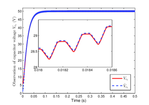
(a) Estimate of $\displaystyle V_{c_{1}}$

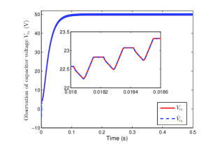
(b) Estimate of $\displaystyle V_{c_{1}}$

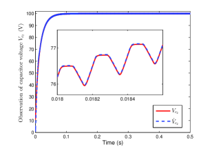
(c) Estimate of $\displaystyle V_{c_{2}}$

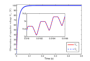
(d) Estimate of $\displaystyle V_{c_{2}}$

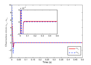
(e) Estimation errors $\displaystyle e_{V_{c_{1}}},e_{V_{c_{2}}}$

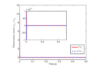
(f) Estimation errors $\displaystyle e_{V_{c_{1}}},e_{V_{c_{2}}}$

Figure 2: Estimate of capacitor voltage $\displaystyle V_{c_{1}},V_{c_{2}}$ and its errors for adaptive-gain SOSML (2(a), 2(c), 2(e)) and Luenberger switched observer (2(b), 2(d), 2(f)), respectively, when the system output is not affected by noise and load variations

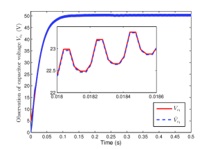
(a) Estimate of $\displaystyle V_{c_{1}}$

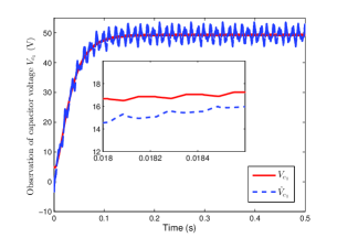
(b) Estimate of $\displaystyle V_{c_{1}}$

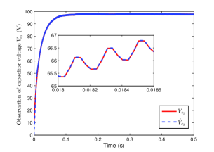
(c) Estimate of $\displaystyle V_{c_{2}}$

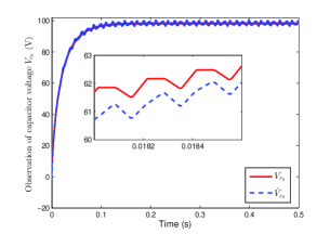
(d) Estimate of $\displaystyle V_{c_{2}}$

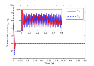
(e) Estimation errors $\displaystyle e_{V_{c_{1}}},e_{V_{c_{2}}}$

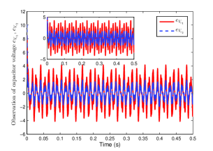
(f) Estimation errors $\displaystyle e_{V_{c_{1}}},e_{V_{c_{2}}}$

Figure 3: Estimate of capacitor voltage $\displaystyle V_{c_{1}},V_{c_{2}}$ and its errors for adaptive-gain SOSML (3(a), 3(c), 3(e)) and Luenberger switched observer (3(b), 3(d), 3(f)), respectively, when the system output is affected by noise and load variations $\displaystyle\hat{R}=1.5R$

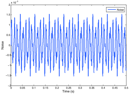
Figure 4: System output noise

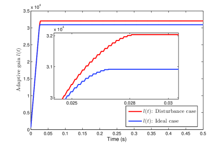
Figure 5: Adaptive law $\displaystyle l(t)$ of the SOSML algorithm

References

- Babaali & Pappas (2005) Babaali, M., & Pappas, G. J. (2005). Observability of switched linear systems in continuous time. In Hybrid systems: Computation and control (pp. 103–117). Springer.
- Bâja et al. (2007) Bâja, M., Patino, D., Cormerais, H., Riedinger, P., & Buisson, J. (2007). Hybrid Control of a Three-Level Three-Cell DC-DC Converter. In American Control Conference (ACC) (pp. 5458–5463). IEEE.
- Bejarano et al. (2010) Bejarano, F., Ghanes, M., & Barbot, J.-P. (2010). Observability and Observer Design for Hybrid Multicell Choppers. International Journal of Control, 83, 617–632.
- Bensaid & Fadel (2001a) Bensaid, R., & Fadel, D. (2001a). Sliding-Mode Observer For Multicell Converters. In Proceedings of Nonlinear Control Systems (NOLCOS), 2001, IFAC (pp. 1396–1401).
- Bensaid & Fadel (2001b) Bensaid, R., & Fadel, M. (2001b). Floating Voltages Estimation In Three-Cell Converters Using a Discrete-Time Kalman Filter. In 32nd Annual IEEE Power Electronics Specialists Conference, PESC. (pp. 327–332).
- Bensaid & Fadel (2002) Bensaid, R., & Fadel, M. (2002). Flying Capacitor Voltages Estimation In Three-Cell Converters Using a Discrete-Time Kalman Filter at One Third Switching Period. In Proceedings of the American Control Conference. (pp. 963–968).
- Besançon (2007) Besançon, G. (2007). Nonlinear Observers and Applications volume 363. Springer Verlag.
- Defaÿ et al. (2008) Defaÿ, F., Llor, A., & Fadel, M. (2008). A Predictive Control With Flying Capacitor Balancing of a Multicell Active Power Filter. IEEE Transactions on Industrial Electronics, 55, 3212–3220.
- Defoort et al. (2011) Defoort, M., Djemaï, M., Floquet, T., & Perruquetti, W. (2011). Robust Finite Time Observer Design for Multicellular Converters. International Journal of Systems Science, 42, 1859–1868.
- Djemaï et al. (2011) Djemaï, M., Busawon, K., Benmansour, K., & Marouf, A. (2011). High-Order Sliding Mode Control of a DC Motor Drive Via a Switched Controlled Multi-Cellular Converter. International Journal of Systems Science, 42, 1869–1882.
- Evangelista et al. (2013) Evangelista, C., Puleston, P., Valenciaga, F., & Fridman, L. (2013). Lyapunov-Designed Super-Twisting Sliding Mode Control for Wind Energy Conversion Optimization. IEEE Transactions on Industrial Electronics, 60, 538–545.
- Gateau et al. (2002) Gateau, G., Fadel, M., Maussion, P., Bensaid, R., & Meynard, T. (2002). Multicell Converters: Active Control and Observation of Flying-Capacitor Voltages. IEEE Transactions on Industrial Electronics, 49, 998–1008.
- Gerry et al. (2003) Gerry, D., Wheeler, P., & Clare, J. (2003). High-Voltage Multicellular Converters Applied to AC/AC Conversion. International Journal of Electronics, 90, 751–762.
- Kang et al. (2009) Kang, W., Barbot, J., & Xu, L. (2009). On the Observability of Nonlinear and Switched Systems. Emergent Problems in Nonlinear Systems and Control, (pp. 199–216).
- Khalil (2001) Khalil, H. K. (2001). Nonlinear Systems. (3rd ed.). Prentice Hall.
- Kouro et al. (2010) Kouro, S., Malinowski, M., Gopakumar, K., Pou, J., Franquelo, L. G., Wu, B., Rodriguez, J., Perez, M. A., & Leon, J. I. (2010). Recent Advances and Industrial Applications of Multilevel Converters. IEEE Transactions on Industrial Electronics, 57, 2553–2580.
- L. Amet, M. Ghanes, J.P. Barbot (2011) L. Amet, M. Ghanes, J.P. Barbot (2011). Direct Control Based on Sliding Mode Techniques for Multicell Serial Chopper. In American Control Conference (ACC), 2011 (pp. 751–756).
- Levant (1998) Levant, A. (1998). Robust Exact Differentiation Via Sliding Mode Technique. Automatica, 34, 379–384.
- Lezana et al. (2009) Lezana, P., Aguilera, R., & Quevedo, D. (2009). Model Predictive Control of an Asymmetric Flying Capacitor Converter. IEEE Transactions on Industrial Electronics, 56, 1839–1846.
- Lienhardt et al. (2007) Lienhardt, A.-M., Gateau, G., & Meynard, T. A. (2007). Digital Sliding-Mode Observer Implementation Using FPGA. IEEE Transactions on Industrial Electronics, 54, 1865–1875.
- Loría & Panteley (2002) Loría, A., & Panteley, E. (2002). Uniform exponential stability of linear time-varying systems: revisited. Systems Control Letters, 47, 13–24.
- M. Ghanes, F. Bejarano and J.P. Barbot (2009) M. Ghanes, F. Bejarano and J.P. Barbot (2009). On Sliding Mode and Adaptive Observers Design for Multicell Converter. In American Control Conference (ACC), 2009 (pp. 2134–2139). IEEE.
- McGrath & Holmes (2007) McGrath, B., & Holmes, D. (2007). Analytical Modelling of Voltage Balance Dynamics for a Flying Capacitor Multilevel Converter. In Power Electronics Specialists Conference, PESC, IEEE (pp. 1810–1816).
- Meradi et al. (2013) Meradi, S., Benmansour, K., Herizi, K., Tadjine, M., & Boucherit, M. (2013). Sliding Mode and Fault Tolerant Control for Multicell Converter Four Quadrants. Electric Power Systems Research, 95, 128–139.
- Meynard et al. (1997) Meynard, T., Fadel, M., & Aouda, N. (1997). Modeling of Multilevel Converters. IEEE Transactions on Industrial Electronics, 44, 356–364.
- Meynard & Foch (1992) Meynard, T., & Foch, H. (1992). Multi-Level Conversion: High Voltage Choppers and Voltage-Source Inverters. In 23rd Annual Power Electronics Specialists Conference (pp. 397–403). IEEE.
- Moreno & Osorio (2008) Moreno, J., & Osorio, M. (2008). A Lyapunov Approach to Second-Order Sliding Mode Controllers and Observers. In 47th IEEE Conference on Decision and Control (CDC) (pp. 2856–2861). IEEE.
- Oettmeier et al. (2009) Oettmeier, F. M., Neely, J., Pekarek, S., DeCarlo, R., & Uthaichana, K. (2009). MPC of Switching in a Boost Converter Using a Hybrid State Model With a Sliding Mode Observer. IEEE Transactions on Industrial Electronics, 56, 3453–3466.
- Perruquetti & Barbot (2002) Perruquetti, W., & Barbot, J. P. (2002). Sliding Mode Control in Engineering volume 11. CRC Press.
- Rech & Pinheiro (2007) Rech, C., & Pinheiro, J. (2007). Hybrid Multilevel Converters: Unified Analysis and Design Considerations. IEEE Transactions on Industrial Electronics, 54, 1092–1104.
- Respondek et al. (2004) Respondek, W., Pogromsky, A., & Nijmeijer, H. (2004). Time Scaling for Observer Design with Linearizable Error Dynamics. Automatica, 40, 277–285.
- Riedinger et al. (2010) Riedinger, P., Sigalotti, M., & Daafouz, J. (2010). On the Algebraic Characterization of Invariant Sets of Switched Linear Systems. Automatica, 46, 1047–1052.
- Rodriguez et al. (2002) Rodriguez, J., Lai, J., & Peng, F. (2002). Multilevel Inverters: a Survey of Topologies, Controls, and Applications. IEEE Transactions on Industrial Electronics, 49, 724–738.
- Vidal et al. (2003) Vidal, R., Chiuso, A., Soatto, S., & Sastry, S. (2003). Observability of Linear Hybrid Systems. Hybrid Systems: Computation and Control, (pp. 526–539).