Spin dynamics of two bosons in an optical lattice site: a role of anharmonicity and anisotropy of the trapping potential

Abstract

We study spin dynamics of two magnetic Chromium atoms trapped in a single site of a deep optical lattice in a resonant magnetic field. Dipole-dipole interactions couple spin degrees of freedom of two particles to their quantized orbital motion. A trap geometry combined with two-body contact s-wave interactions influence a spin dynamics through the energy spectrum of the two atom system. Anharmonicity and anisotropy of the site results in a ‘fine’ structure of two body eigenenergies. The structure can be easily resolved by weak magnetic dipole-dipole interactions. As an example we examine the effect of anharmonicity and anisotropy of the binding potential on demagnetization processes. We show that weak dipolar interactions provide a perfect tool for a precision spectroscopy of the energy spectrum of the interacting few particle system.

I Introduction

Dipolar magnetic interactions couple a spin of two particles to their orbital motion in the trap Ueda_review . A particular example of the spin dynamics driven by the dipole-dipole interactions and coupled to the orbital motion of the entire ferromagnetic sample is known as the Einstein-de Haas effect (EdH). The effect is a macroscopic illustration of the fact that spin contributes to the total angular momentum of the system on the same footing as the orbital angular momentum.

In the original experiment Richardson ; EdH1 ; EdH2 a rotation of a ferromagnetic rode was observed when a relative orientation of a magnetic field (forcing a magnetization of the sample along the field axis) and a magnetic moment of the sample had been inverted. The rotation results form the fact that atomic spins adjust to a new orientation of the magnetic field and conservation of the $z$-component of the total angular momentum forces the orbital angular momentum of the sample to compensate for the change of the spin orientation. The orbital angular momentum has to depart from its initial zero value. The EdH effect strongly relays on the dipole-dipole interactions. These interactions, due to their anisotropy do not have to conserve the orbital angular momentum. Only in the presence of the dipolar interactions initially non-rotating system can start to rotate.

The EdH effect was also predicted for ultra cold trapped atomic gases Ueda_1 ; Santos ; KG . Here it serves as a spectacular manifestation of the dipole-dipole interactions of atomic magnetic moments. This leads to a nontrivial dynamics coupling orbital motion and atomic spin. Spin dynamics due to the dipole-dipole interactions is inevitably associated with an excitation of orbital motion of an atom in the trap. The motion is quantized, there is therefore an energy gap separating initial and final states of a different magnetization. The quantization of orbital energy of atoms significantly effects a spin dynamics. This has been noticed in Swislocki .

Two scenarios are possible depending on a ratio of the energy gap to the dipolar energy. For a relatively dense gas of polarized Chromium atoms ($10^{15}{\rm cm}^{-3}$) initially in $S=3,m_{S}=3$ state and for relatively weak harmonic traps ($\omega\simeq 2\pi\times 100{\rm Hz}$), the dipolar energy can exceed the excitation gap what makes the spin dynamics possible. The atoms are transfered first to $m_{S}=2$ state and then, due to higher order processes and the contact interactions, to other magnetic components Ueda_1 .

Situation is different in optical lattices or in a case of species with a small magnetic moment, such as ferromagnetic Rubidium. In general if the dipolar energy is much less than the orbital excitation energy then spin dynamics is suppressed due to the energy conservation.

This obstacle can be overcome. As shown in Swislocki the energies of both involved states can be tuned due to a Zeeman effect. The atoms prepared in $m_{S}=3$ state can be transferred to initially unoccupied $m_{S}=2$ components on the expense of the Zeeman, instead of the dipolar energy. In axially symmetric traps the phase of the $m_{S}=2$ atoms’ wavefunction displays a characteristics vortex-like defect signifying an orbital angular momentum in a final state. This scenario has been studied in the mean field limit, for a three component Rubidium spinor condensate Swislocki . It has been shown that different final states, all involving vortex-like excitation, can be populated via the dipolar processes of the EdH type. Even highly excited trap states can be reached if energy and angular momentum conservation are met by an appropriate choice of the resonant magnetic field.

Energy conservation makes the weak dipolar interactions highly sensitive, selective and tunable by means of the external magnetic field. This requires however, a very high precision in control of both a value and a direction of the field applied. Stabilization of the ultra weak magnetic field with precision below 1 mG is required for Chromium atoms Bruno_1 . The proposal exists suggesting that the time dependent magnetic fields might relax these constrains Brewczyk . The resonant character of demagnetization of initially polarized Chromium atoms in an optical lattice has been demonstrated recently Tolra_rezonanse .

The EdH effect was also suggested as a mechanism to create excited orbital states in the optical lattice Pietraszewicz . The mechanism leads also to an interesting physics described by Bose-Hubbard models with two spin species occupying different Wannier states. The axial symmetry of a single lattice site was assumed. This assumption seems to be quite obvious and is frequently used even in more ‘exotic’ situations Vincent .

In this paper we want to reexamine carefully the role of the harmonic approximation and show its consequences on the spin dynamics, in particular for situations when higher orbital Wannier states are involved. We study elementary processes driven by the dipolar interactions with two atoms trapped in a single site of a high square optical lattice. Such a scenario was considered in You where it has been shown that $100\%$ efficient resonant transfer of atoms to the orbital state is possible. We show that the anharmonicity of the binding potential plays a very important role. In the context of ultracold atoms the effect of anharmonicity was discussed previously in Colin ; Larson .

The paper is organized as follows. In section II we define the Hamiltonian of the system as well as all approximations and model parameters. Then in section III we discuss a resonant dipolar coupling allowing for efficient spin transfer in the channel where spin projection of only one atom changes by one quantum. In section IV we present a detailed analysis of processes when spins of both interacting atoms change by one quantum each (the spin of the doublon changes by two quanta). In particular we take into account separately the effect of anharmonicity of the trapping potential and, finally, both effects of anisotropy and anharmonicity of a single site of a square optical lattice. In section V we compare our results with experimental data of Tolra_rezonanse . Final remarks are presented in section VI.

II The model

II.1 The Hamiltonian

We study a simple system of two Chromium ⁵²Cr atoms in the $S=3$ ground state in a single site of a 2D square optical lattice created by a two pair of counter propagating laser beams of wavelength $\lambda$ and momentum $k=2\pi/\lambda$. A confinement in the z-direction is provided by a harmonic potential of frequency $\Omega_{z}$. We assume that the lattice depth is so big that we can neglect tunneling to the neighboring sites. Through the paper we use the lattice units, i.e. the distance is measured in $1/k=\lambda/2\pi$, all energies in units of the recoil energy $E_{R}=(\hbar k)^{2}/(2M)$, where $M$ is the atomic mass. The units of time and frequency are $\hbar/E_{R}$ and $E_{R}/\hbar$ respectively. The magnetic field unit is $B_{0}=E_{R}/(g\mu_{B})$, where $\mu_{B}$ is the Bohr magneton and $g=2$ is a Lande factor.

The Hamiltonian of the system has the following form:

$${\cal H} =\sum_{i=1}^{2}\left[-\nabla_{i}^{2}+V_{0}(\sin^{2}x_{i}+\sin^{2}y_{i})+\kappa^{2}z_{i}^{2})\right]$$

$$+\delta(\boldsymbol{r}_{1}-\boldsymbol{r}_{2})\sum_{{\cal S}=0}^{2S}g_{{\cal S}}\sum_{{\cal M}=-{\cal S}}^{\cal S}|{\cal S},{\cal M}\rangle\langle{\cal S},{\cal M}|$$

$$+\left(\boldsymbol{S}_{1}+\boldsymbol{S}_{2}\right)\cdot\boldsymbol{B}$$

$$+{d^{2}}\frac{\boldsymbol{S}_{1}\cdot\boldsymbol{S}_{2}-3(\boldsymbol{n}\cdot\boldsymbol{S}_{1})(\boldsymbol{n}\cdot\boldsymbol{S}_{2})}{|\boldsymbol{r}_{1}-\boldsymbol{r}_{2}|^{3}},$$ (1)

where $\boldsymbol{r}_{i}=(x_{i},y_{i},z_{i})$ and $\boldsymbol{S}(i)$ are positions and spin operators of the $i$-th atom respectively. By $\boldsymbol{n}=\boldsymbol{r}/r$ we denote the unit vector in the direction of $\boldsymbol{r}=\boldsymbol{r}_{1}-\boldsymbol{r}_{2}=(x,y,z)$. Spin operators are represented by the spin $7\times 7$ matrices. To describe the contact two-body interactions, which depend on the total spin of both atoms, we use the molecular basis in the spin space:

$$|{\cal S},{\cal M}\rangle=\sum_{m_{1},m_{2}}(S,m_{1};S,m_{2}|{\cal S},{\cal M})|S,m_{1}\rangle|S,m_{2}\rangle,$$ (2)

where $|{\cal S},{\cal M}\rangle$ is a two particle spin state with the total spin ${\cal S}$ and the projection $\cal M$. The symbol $(S,m_{1};S,m_{2}|{\cal S},{\cal M})$ is the Clebsch-Gordan coefficient and $|S,m_{i}\rangle$ describes the spin state of the single atom of spin $S$ and its projection $m_{i}$. Note that due to the symmetry the total spin of the doublon, $\cal S$ can take only even values, ${\cal S}=0,2,4,6$. The parameter $\kappa$ is: $\kappa=(\hbar\Omega_{z})/(2E_{R})$. The strength of the contact interactions $g_{{\cal S}}$ is proportional to the s-wave scattering length $a_{{\cal S}}$ in the given $\cal S$-channel:

$$g_{{\cal S}}=8\pi ka_{{\cal S}}.$$ (3)

Finally the dimensionless dipole-dipole interaction strength reads $d^{2}=\mu_{0}/(4\pi)(g\mu_{B})^{2}(k^{3}/E_{R})$, where $\mu_{0}$ is the magnetic constant.

The physical meaning of all the terms in the Hamiltonian Eq.(II.1) is straightforward. The first line corresponds to the single particle energy, $H_{0}$, including both kinetic and potential energies, while the second line describes the contact interactions between particles, $H_{C}$. In principle, the contact interactions can lead to a spin dynamics. In this paper we assume that initially both atoms are prepared in the ground state of the lattice site in the presence of sufficiently strong magnetic field to assure a ferromagnetic polarization of the system. The initial spin state of the doublon is $|{\cal S},{\cal M}\rangle=|6,6\rangle$. In such a situation the spin dynamics is driven, at least initially, by the dipolar interactions only. The external magnetic field, the third line of Eq.(II.1), describes the linear Zeeman shift of single particles energies, $H_{Z}$. The magnetic field allows for tuning of relative energies of the two atoms system. In this paper we assume that the magnetic field is align along the vertical $z$-direction, perpendicular to the 2D lattice plane. Finally, the last line of Eq.(II.1) corresponds to the energy of the dipole-dipole interactions of both atoms, $H_{D}$. The total Hamiltonian is the sum $H=H_{0}+H_{C}+H_{Z}+H_{D}$.

We examine the dipolar terms in more details stressing their role on the spin dynamics. The elementary processes driven by the Hamiltonian $H_{D}$ can be casted into three classes.

1. Collisions not changing orbital angular momentum of the doublon, $\Delta{\cal L}_{z}=0$, where ${\cal L}_{z}$ is the $z$-component of the total orbital angular momentum of the pair. These collisions are governed by the term whose spatial dependence has the form:

$$h_{0}=\frac{d^{2}}{r^{3}}\left(1-\frac{3z^{2}}{r^{2}}\right),$$ (4)

where and $r=|\boldsymbol{r}|$. Note that this term has to be multiplied by the appropriate operator acting in the spinor space:

$$s_{0}=S_{z}(1)S_{z}(2)-{1\over 4}\left(S_{+}(1)S_{-}(2)+S_{-}(1)S_{+}(2)\right).$$ (5)

The $S_{\pm}(i)=S_{x}(i)\pm iS_{y}(i)$ operator rises ($+$) or lowers ($-$) the magnetic quantum number of the $i$-th atom by one quantum. The rising and lowering operators fulfill the commutation relations for the spin, i.e $[S_{+}(k),S_{-}(j)]=2iS_{z}(j)\delta_{kj}$. Note, that the spinor term $s_{0}$ does not change the magnetization of the doublon, $\Delta{\cal M}=0$. The dipolar interaction with $\Delta{\cal L}_{z}=0$ are:

$$H_{d0}=h_{0}\cdot s_{0}$$ (6)

$H_{d0}$ evidently conserves the total angular momentum along the $z$-axis, $\Delta{({\cal L}_{z}+{\cal M})}=0$.

2. Collisions changing the $z$-component of the orbital angular momentum of the doublon by one quantum, $\Delta{\cal L}_{z}=\pm 1$. These processes originate from the term of the following spatial dependence:

$$h_{\pm 1}=-\frac{3d^{2}}{2r^{3}}\frac{z(x\pm iy)}{r^{2}}.$$ (7)

The upper sign corresponds to $\Delta{\cal L}_{z}=1$, while the lower sign to $\Delta{\cal L}_{z}=-1$. This spatial term, $h_{\pm 1}$, has to be assisted by the corresponding spinor term:

$$s_{\mp 1}=S_{z}(1)S_{\mp}(2)+S_{\mp}(1)S_{z}(2).$$ (8)

The upper sign corresponds to processes with $\Delta{\cal M}=-1$ , while the lower sign to the processes with $\Delta{\cal M}=+1$. The dipolar Hamiltonian describing processes with $\Delta{\cal L}_{z}=\pm 1$ is a product of the spatial and the spinor terms:

$$H_{d1}=h_{+1}\cdot s_{-1}+h_{-1}\cdot s_{+1},$$ (9)

and clearly $\Delta{({\cal L}_{z}+{\cal M})}=0$.

3. Collisions changing the $z$-component of the orbital angular momentum of the doublon by two quanta, $\Delta{\cal L}_{z}=\pm 2$ . These processes originate from the term of the following spatial dependence:

$$h_{\pm 2}=-\frac{3d^{2}}{4r^{3}}\frac{(x\pm iy)^{2}}{r^{2}},$$ (10)

which is accompanied by the spin term which changes the spin projection of the doublon by $\Delta{\cal M}=\mp 2$:

$$s_{\mp 2}=S_{\mp}(1)S_{\mp}(2).$$ (11)

The dipolar Hamiltonian describing processes with $\Delta{\cal L}_{z}=\pm 2$ is a product of the spatial and the spinor terms:

$$H_{d2}=h_{+2}\cdot s_{-2}+h_{-2}\cdot s_{+2}.$$ (12)

Clearly the $z$-component of the total angular momentum of the doublon $\Delta{({\cal L}_{z}+{\cal M})}=0$ is conserved.

This way we decomposed the dipolar interactions into different terms:

$$H_{D}=H_{d0}+H_{d1}+H_{d2},$$ (13)

depending on the effect each term has on the orbital (or equivalently the spin) dynamics of the atom pair.

II.2 General considerations

To start with we assume that the external potential near the center of the site at ${\boldsymbol{r}}=0$ can be approximated by the harmonic one. We keep only the lowest order terms in the expansion of the potential in Eq.(II.1):

$$V_{tr}=V_{0}(x^{2}+y^{2})+\kappa^{2}z^{2}$$ (14)

The potential is both harmonic and axially symmetric with effective frequencies $\Omega_{\perp}=\omega_{x}=\omega_{y}=2\sqrt{V_{0}}$ and $\Omega_{z}=2\kappa$. The aspect ratio is $\Omega_{z}/\Omega_{\perp}=\kappa/\sqrt{V_{0}}$.

In the following we assume that initially both atoms are in the ground state of the external trap in the two body $|{\cal S}=6,{\cal M}=6\rangle$ spin state, what corresponds to a fully polarized system with the both atoms in $m=3$ state. The energy of the doublon is equall to a sum of single particle and contact energies. The initial orbital state $\Psi_{\rm ini}({{\bf r}_{1}},{{\bf r}_{2}})=\langle{{\bf r}_{1}},{{\bf r}_{2}}|{\rm ini}\rangle$ does not depend on the angles of the vectors $\bf{r_{1}}$ and $\bf{r_{2}}$:

$$\Psi_{\rm ini}({{\bf r}_{1}},{{\bf r}_{2}})=\phi_{00}(x_{1},y_{1})\varphi_{0}(z_{1})\phi_{00}(x_{2},y_{2})\varphi_{0}(z_{2}),$$ (15)

where $\phi_{00}(x,y)\varphi_{0}(z)$ is the ground state of the harmonic trap. In order to stress that the axial wavefunction, $\varphi_{0}(z)$, corresponds to a different trap frequency we separated out the axial term.

To analyze further approximations we use the realistic parameters related to experiments of Bruno_1 . We assume that the optical lattice is created by the laser light of the wavelength of $532$nm, which gives the unit of distance to be $84,67$nm. For Chromium ⁵²Cr ($M\simeq 87\times 10^{-27}$kg) the recoil energy is $E_{R}/\hbar\simeq 2\pi\times 13,5{\rm kHz}$. A typical height of the potential barrier is $V_{0}=25E_{R}$ what corresponds to $V_{0}/\hbar=2\pi\times 336{\rm kHz}$ for which the characteristic trap frequency is $\Omega_{\perp}=10E_{R}/\hbar=2\pi\times 135{\rm kHz}$. We assume that the axial frequency is $\Omega_{z}=16E_{R}/\hbar=2\pi\times 218{\rm KHz}$.

These parameters lead to a characteristic size of the system of the order of the harmonic oscillator lengths $a_{\perp}=38{\rm nm}$ and $a_{z}=30{\rm nm}$. With two atoms per site the atom density is about $n_{0}\sim 2.8\times 10^{15}{\rm cm}^{-3}$. Corresponding contact interaction in $S=6$ channel is $U_{C}/\hbar\sim 2\pi\times 18.9{\rm kHz}$ while the dipolar interaction $E_{D}/\hbar\sim d^{2}S\sim 2\pi\times 0.37{\rm kHz}$.

The dipolar energy is the smallest energy scale. Thus we can ignore the term of dipolar interactions which does not change a total magnetization of both colliding atoms, i.e. we neglect processes with $\Delta{\cal M}_{z}=0$. The term leads only to small, negligible corrections to the contact interactions.

Clearly, the dipolar interactions leading to a spin dynamics assisted by an inevitable transfer of atoms to excited states of the trap are suppressed by the energy conservation because $\hbar\Omega_{\perp}>>E_{D}$. The spin dynamics activates if the energy gap is compensated by the Zeeman energy. To shift the relative energies of $m=3$ and $m=2$ components by the amount of $\hbar\Omega_{\perp}$ the magnetic field equal to $B_{tr}=48.2$mG is needed. Similarly, the Zeeman energy compensating for the contact interactions is related to the magnetic field $B_{C}\sim 6.75$mG, while the dipolar energy corresponds to $B_{D}\sim 25.7\mu$G. Extremely precise control of bothL: the direction and the value of the magnetic field is necessary to control the spin dynamics in the trap. This makes a great challenge for experiments.

For the initial axially symmetric ground state $\Phi_{\rm ini}=\langle{\rm r}_{1},{\rm r}_{2}|{\rm ini}\rangle$ the processes with $\Delta{\cal M}_{z}=-1$ and $\Delta{\cal M}_{z}=-2$ lead to two different orbital states of the doublon. In the lowest order of the perturbation in the dipolar interactions, the angular dependence of the two atoms’ relative wavefunction (coupled to the ground state by dipolar interactions) is determined by the angular dependence of the dipolar terms, Eqs.(7), (10). The state excited due to $\Delta{\cal M}_{z}=-1$ dipolar process has energy of the order of $\Omega_{\perp}+\Omega_{z}$ , while the energy of the state reached by the system via the second channel, $\Delta{\cal M}_{z}=-2$, is $2\Omega_{\perp}$. If $(\Omega_{z}-\Omega_{\perp})$ is much larger than the dipolar energy then by matching the resonance condition one can activate selectively the first or the second channel (not both of them). Therefore we will analyze the process with $\Delta{\cal M}_{z}=-1$ and $\Delta{\cal M}_{z}=-2$ separately.

Our general strategy is to find the lowest energy state which is coupled by the dipole-dipole interactions to the $|{\rm ini}\rangle$ state as it follows directly from the structure of the dipolar Hamiltonian. At this step we determine a single particle basis which is needed to describe all relevant two-body states. Then we diagonalize the full Hamiltonian $H$ in the chosen basis and find eigenenergies and eigenvectors of the doublon. At every resonance there exists an eigenvector of the Hamiltonian which is an equal-amplitude superposition of the initial and the final state. The two states forming the superposition are coupled by the dipolar interaction.

Alternatively, the physical insight can be gained with the help of a perturbative analysis. The state determined by the structure of the dipole-dipole term is not necessarily the eigenstate of the single particle and the contact Hamiltonian. The goal is to decompose this state in the eigenstate basis of $H_{0}+H_{Z}+H_{C}$. A number of dipolar resonances equals to a number of different eigenstates involved in the decomposition. Each component has different eigenenergy and therefore becomes resonant at a different magnetic field.

To the ‘zero order’ approximation the energy of a final state - the state accessible by the dipolar interactions – is given by the sum of the single particle energies (i.e. $\Omega_{\perp}+\Omega_{z}$ in the $\Delta{\cal M}_{z}=-1$ channel or $2\Omega_{\perp}$ in $\Delta{\cal M}_{z}=-2$ channel). The single particle energy gives an estimation of the resonant magnetic field. However, anharmonicity and anisotropy shift one-particle energies and the contact interactions couple them. These effects result in a splitting of energies of different components of the final states accessible via the dipole-dipole interactions i.e. in an appearance of a fine resonant structure.

The strength of the resonant dipole-dipole interactions can be characterized by the self energy of the initial $|{\rm ini}\rangle$ state of energy $E_{0}(B)$:

$$E_{sf}(B)=\sum_{i}\frac{|D_{i}|^{2}}{\sqrt{\left(\frac{E_{i}(B)-E_{0}(B)}{2}\right)^{2}+|D_{i}|^{2}}}.$$ (16)

$|\Psi_{i}\rangle$ and $E_{i}(B)$ are ‘bare’ eigenstates and eigenenergies of the two-body Hamiltonian without the dipolar interactions, $(H_{0}+H_{C}+H_{Z})|\Psi_{i}\rangle=E_{i}(B)|\Psi_{i}\rangle$, while $D_{i}=\langle{\rm ini}|H_{D}|\Psi_{i}\rangle$ is the dipole-dipole interaction matrix element. The self energy contains a contribution from a virtual transfer of the doublon from $|{\rm ini}\rangle$ to the intermediate $|\Psi_{i}\rangle$ state. Evidently, this process contributes only at the vicinity of the resonance, where:

$$E_{i}(B_{res})-E_{0}(B_{res})\simeq D_{i},$$ (17)

The particular form of the self energy results from the fact, that at every resonance we deal with a two level system, and then the denominator in Eq.(16) gives the energy shift of the $|{\rm ini}\rangle$ state.

III Dipolar processes with $\Delta{\cal M}_{z}=-1$

The spatial part of the lowest energy state of the doublon accessible via the dipole-dipole interactions in $\Delta{\cal M}_{z}=-1$ channel is $\sim z(x+iy)$, where $x,y,z$, are relative coordinates of two atoms. This state is created by a two-particle operator:

$$v_{1}^{\dagger}=\frac{1}{2}\left(p^{\dagger}_{z}\left(p^{\dagger}_{x}+ip^{\dagger}_{y}\right)-s^{\dagger}\left(d^{\dagger}_{xz}+id^{\dagger}_{yz}\right)\right),$$ (18)

acting on the particle vacuum. The bosonic operators in the above formula create a particle in the one of the following states of the harmonic oscillator: $s^{\dagger}$ – in the ground state $\phi_{00}(x,y)\varphi_{0}(z)$, $p^{\dagger}_{x}$, $p^{\dagger}_{y}$ – in one of the two $p$-shell states: $\phi_{10}(x,y)\varphi_{0}(z)$ or $\phi_{01}(x,y)\varphi_{0}(z)$ respectively, $d^{\dagger}_{xz}$ and $d^{\dagger}_{yz}$ – in the $d$-shell states – $\phi_{10}(x,y)\varphi_{1}(z)$ or $\phi_{01}(x,y)\varphi_{1}(z)$. $\varphi_{1}(z)$ is the first excited state in the axial direction. The operator $v_{1}^{\dagger}$ allows for a compact representation of the ‘vortex’ state with ${\cal L}_{z}=1$. The vortex is created in a relative coordinate space of the doublon. The first term in Eq.(18) describes the state in which one atom takes one excitation quanta in the axial direction, while the second carries the vortex like excitation. The second term corresponds to a process in which one atom experiences both types of excitations while the second atom is a spectator (at least as the spatial wavefunction is considered).

The operator $v^{\dagger}_{1}$ defines only a spatial part of ${\cal L}_{z}=1$ vortex state:

$$|{\cal L}_{1}\rangle=v_{1}^{\dagger}|0\rangle.$$ (19)

To account for a total state of the system including spin degrees of freedom, the $|{\cal L}_{1}\rangle$ state has to be multiplied by a totally symmetric spinor component with one atom in $|m=3\rangle$ and the other in $|m=2\rangle$ spin states. The final state of the system is:

$$|{\cal F}\rangle=\frac{1}{\sqrt{2}}\left(|3\rangle|2\rangle+|2\rangle|3\rangle\right)|{\cal L}_{1}\rangle.$$ (20)

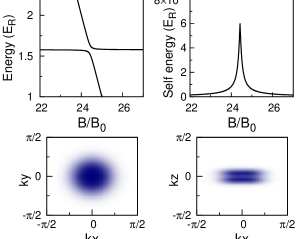
Figure 1: Harmonic trap – dipolar resonances with $\Delta{\cal M}_{z}=-1$. Left upper panel: the excitation energy of the two particle system in the harmonic trap as a function of an external magnetic field. The horizontal line at small $B$ corresponds to the $|{\rm ini}\rangle$ state with both atoms fully polarized $|3\rangle|3\rangle$. Only the lowest energy state $|{\cal L}_{1}\rangle$, the one which is coupled to the $|{\rm ini}\rangle$ state by $\Delta{\cal M}_{z}=-1$ dipole-dipole interaction term is shown. Notice avoided crossing. Right upper panel: a single maximum in the self-energy curve (right upper panel) signifying strong coupling of both involved states at resonant magnetic field. Lower panel: reduced single particle density matrix component (the diagonal element with magnetization $m=2$) of the state $|{\cal L}_{1}\rangle$; left panel – density cut at $xy$ plane for $z=1/\sqrt{\kappa}$, right panel – density at $xz$ plane ($y=0$).

The most important observation is that the contact interactions vanish in the $|{\cal L}_{1}\rangle$ state because its wavefunction vanishes identically if ${\bf r}_{1}={\bf r}_{2}$, i.e. $\langle{\bf r},{\bf r}|{\cal L}_{1}\rangle=0$. This state is not coupled by the contact interaction to any other state of the doublon in the trap. It is therefore the eigenstate of both the single particle and the contact Hamiltonians. The dipole-dipole interactions couple efficiently the state to the initial one if energies of the involved states do match. This can happen if $E_{{\cal L}_{1}}=\Omega_{\perp}+\Omega_{z}+(2+3)B$ equals to the energy of the initial state $E_{ini}=U_{33}+2(3B)$. The resonance condition is met at the magnetic field $B_{res}=(\Omega_{z}+\Omega_{\perp})-U_{33}$. $U_{33}=(g_{6}/8)\sqrt{\Omega_{\perp}^{2}\Omega_{z}/\pi^{3}}$ is the contact interaction of two particles in $m=3$ state and the ground state of the harmonic potential.

The state is also robust if anharmonicity of a the lattice site potential is taken into account. In our case the lattice potential depends only on $x$ and $y$ coordinates. The $z$-direction separates. This fact has very important consequences: $d_{xz}$ and $d_{yz}$ states are separable. Their single particle energies are sum of $p$-band energies. For this reason the two components of the $|{\cal L}_{1}\rangle$ state, i.e. the one with two excited particle and the second with only one excited particle, are degenerate. Anharmonicity of the lattice potential results in an equal shifts of both components of the $|{\cal L}_{1}\rangle$ state and does not lift their degeneracy. Moreover, this conclusion holds even when axial symmetry of the external potential is substituted by the $Z_{2}$ symmetry of the single site of the lattice. $Z_{2}$ symmetry is sufficient to assure the degeneracy of $p_{x}$ and $p_{y}$ orbitals. The only effect of the lattice potential is to shift the value of the resonant magnetic field.

The latter will not be true if $p_{x}$ and $p_{y}$ orbitals have different energies. In such a case the $|{\cal L}_{1}\rangle$ state will be a superposition of two eigenstates of different energies, and each component could be separately addressed in a dipolar process by an appropriate tuning of the magnetic field. Two resonances will be observed in such a case.

Diagonalization of the full Hamiltonian in the oscillatory or Wannier basis supports the above discussion. We find only one low energy state coupled by the dipole-dipole interactions to the initial one. In Fig.1 we show eigenenergies of the two states. The avoided crossing, signifying the dipolar coupling is clearly visible. In the lower panel the single particle density in $m=2$ spin component is shown ($xy$ and $xz$ cuts). Note the node in $z=0$ plane what is typical for the first excited state in the axial direction. The single particle density does no resemble the structure typical for a single particle vortex state. This is because the vortex is created in the relative coordinates of two particles. In Fig.1 (upper right panel) the self energy of the initial state is plotted. The hight of the resonant peak indicates the value of the dipolar matrix element coupling the states. If the magnetic field is tuned to the resonant value the system will perform Rabi oscillations between the initial and the final state. The final state reached via the dipole-dipole interactions is highly entangled, Eq.(20).

IV Dipolar processes with $\Delta{\cal M}_{z}=-2$

IV.1 Harmonic trap

In this section we examine collisions changing magnetization of the system by two quanta, $\Delta{\cal M}_{z}=-2$. The two interacting particles, trapped in a harmonic potential, go simultaneously from $|3\rangle|3\rangle$ to $|2\rangle|2\rangle$ spin state. Spatial part of the relative wavefunction in the lowest accessible final state must be proportional to $\sim(x+iy)^{2}$ in order to compensate for a decrease of the spin of the doublon by two quanta. This is the wavefunction of a doubly charged vortex in the relative coordinates space. This simple state (normalized) if written in the harmonic basis looks quite complicated, so it is convenient to describe it using the second quantization picture. The ‘vortex’ state is created by the two-body operator $v^{\dagger}_{2}$:

$$v^{\dagger}_{2} = \frac{1}{2\sqrt{2}}\left(s^{\dagger}\left(d^{\dagger}_{xx}+i\sqrt{2}d^{\dagger}_{xy}-d^{\dagger}_{yy}\right)\right.$$

$$\left.-\frac{1}{\sqrt{2}}\left((p^{\dagger}_{x})^{2}+i2p^{\dagger}_{x}p^{\dagger}_{y}-(p^{\dagger}_{y})^{2}\right)\right).$$

In addition to defined previously bosonic operators creating a particle in $s$ and $p$ shells we define the $d$ shell operators: $d^{\dagger}_{xx}$, $d^{\dagger}_{yy}$, and $d^{\dagger}_{xy}$ creating a particle in the second excited state of a harmonic oscillator potential, i.e. $\phi_{20}(x,y)\varphi_{0}(z)$, $\phi_{02}(x,y)\varphi_{z}(0)$, and $\phi_{11}(x,y)\varphi_{0}(z)$ respectively.

The first line describes the state with one particle in the ground $s$ state and the second particle in the excited $d$-shell state with ${\cal L}_{z}=2$. The second line corresponds to a state with two particles occupying the $p_{x}+ip_{y}$ vortex. Let us note that introduced here states, abbreviated by $s$, $p_{x}$, $p_{y}$, $d_{xx}$, $d_{yy}$, and $d_{xy}$, span a basis of the orbital states which is sufficient to describe the lowest dipolar excitations in $\Delta{\cal M}_{z}=-2$ channel.

The orbital basis has to be completed by the spin states. These are the initial $|3\rangle|3\rangle$ and the final $|2\rangle|2\rangle$ states. The further spin dynamics due to the spin dependent contact interactions can subsequently induce a transition from $|2\rangle|2\rangle$ to $(|1\rangle|3\rangle+|3\rangle|1\rangle)/\sqrt{2}$ state. However, the process can be suppressed due to the energy mismatch if $m=2$ state is shifted by light. Therefore for a moment we neglect contact spin-changing collisions.

We diagonalize the total Hamiltonian Eq.(II.1) in the basis of the two particle states spanned by the introduced above single particle $s$, $p$ and $d$ orbitals in the initial $m=3$ and the final $m=2$ spin component for different values of an external magnetic field.

However to gain an insight into physical processes involved we shall describe the results using perturbative approach with a dipole-dipole interaction energy as a small parameter. First we diagonalize the single particle and contact Hamiltonian $H_{0}+H_{Z}+H_{C}$. As expected, the state $|{\cal L}_{2}\rangle$, defined as:

$$|{\cal L}_{2}\rangle=v^{\dagger}_{2}|0\rangle,$$ (22)

is the eigenstate of $H_{0}+H_{Z}+H_{C}$. Moreover, the contact energy vanishes in this state. This is a unique feature of the harmonic potential and has some important consequences on the spin dynamics as it will be shown later. The energy of this state $E_{{\cal L}_{2}}=2\Omega_{\perp}+2(2B)$ equals to the energy of the initial state $E_{ini}=U_{33}+2(3B)$ at the magnetic field $B_{res}=\Omega_{\perp}-U_{33}/2$. $U_{33}=(g_{6}/8)\sqrt{\Omega_{\perp}^{2}\Omega_{z}/\pi^{3}}$ is the contact interaction of two particles in $m=3$ state and the ground state of the harmonic potential.

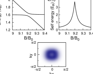
Figure 2: Harmonic trap – dipolar resonances with $\Delta{\cal M}_{z}=-2$. Left upper panel: excitation energy of the two particle system in the harmonic trap as a function of an external magnetic field. The horizontal line at small $B$ corresponds to the $|{\rm ini}\rangle$ state with both atoms fully polarized $|3\rangle|3\rangle$. Notice avoided crossing. Right upper panel: a single maximum in the self-energy curve signifying strong coupling of both involved states at the resonant magnetic field. Lower panel: reduced single particle density (in $xy$ plane) of $|{\cal L}_{2}\rangle$ state coupled to the $|{\rm ini}\rangle$ state.

Evidently, by the construction, $|{\cal L}_{2}\rangle$ is coupled to the initial state: $D=\langle{\cal L}_{2}|h_{+2}|{\rm ini}\rangle\neq 0$. By diagonalization of the full Hamiltonian with the dipole-dipole term included, we indeed find that $|{\cal L}_{2}\rangle$ state is the only one coupled to $|{\rm ini}\rangle$ state by the dipole-dipole interactions. The two coupled states, $|\rm ini\rangle$ and $|{\cal L}_{2}\rangle$ form a two level system. Its eigenenergies depend on the value of the external magnetic field. They are shown in Fig.2. The visible avoided crossing corresponds to the resonance. Obviously there are other resonant states, not included in our basis, which are coupled by the dipolar interactions to the initial state. This coupling takes place, however at higher magnetic fields which we do not consider here.

In the upper right panel of Fig.2 we show the self energy of the $|{\rm ini}\rangle$ as a function of the magnetic field. The self energy reaches maximum at the resonance. The magnitude of $E_{sf}$ at the resonance is equal to $|D|$. Similarly, a width of the resonance is also equal to $|D|$.

Weakness of the dipolar coupling allows for a precise tuning of the two atom system. Initial population of the $m=3$ state will oscillate periodically between two coupled states with a Rabi frequency proportional to the dipolar energy $D$. At half of the period all the population will be transferred to the $m=2$ state, $|{\cal L}_{2}\rangle$. The single particle density corresponding to this state is shown in the lower panel of Fig.2. Note a shallow minimum at the trap center. The vortex $|{\cal L}_{2}\rangle$ state is a vortex in the relative coordinate space. This is not a vortex in the reduced one-particle space.

Finally we return to the observation that the contact interaction in $|{\cal L}_{2}\rangle|2\rangle|2\rangle$ state vanishes, i.e. $U_{22}=g_{22}\langle{\cal L}_{2}|\delta({\bf r}_{1}-{\bf r}_{2})|{\cal L}_{2}\rangle=0$, where $g_{22}=(6g_{6}+5g_{4})/11$. This is because the two body wavefunction of this state vanishes if ${\bf r}_{1}={\bf r}_{2}$. The contact interactions leading to the transfer of one atom to $m=3$ and the second one to $m=1$ state, $U_{22,31}=g_{22,31}\langle{\cal L}_{2}|\delta({\bf r}_{1}-{\bf r}_{2})|{\cal L}_{2}\rangle=0$, also vanishes, where $g_{22,31}=\sqrt{30}/11(g_{6}-g_{4})$. Therefore, in the harmonic axially symmetric trap the spin dynamics of the $|{\cal L}_{2}\rangle|2\rangle|2\rangle$ state due to the contact spin changing collisions is forbidden. There is no need to detune $m=2$ state with respect to $m=3$ and $m=1$ states to prevent contact spin changing collisions. This fact is in a contradiction with experiments with Chromium atoms in an optical lattice Bruno_1 and clearly indicates that the harmonic approximation does not describe correctly the spin dynamics in the optical lattices.

IV.2 Anharmonic trap

If in the expansion of a the lattice site potential we keep the higher order terms then we get a potential which is neither harmonic nor axially symmetric:

$$V({\bf r})=V_{0}\rho^{2}-\frac{1}{3}V_{0}\rho^{4}+\kappa^{2}z^{2}+\frac{2}{3}V_{0}x^{2}y^{2},$$ (23)

where $\rho^{2}=x^{2}+y^{2}$. The second term $\sim\rho^{4}$ introduces anharmonicity while the last term brakes the axial symmetry. To separate effects of anharmonicity from effects of anisotropy we neglect the last term and consider the model anharmonic potential

$$V({\bf r})=V_{0}\rho^{2}-\frac{1}{3}V_{0}\rho^{4}+\kappa^{2}z^{2}.$$ (24)

The combined effect of anharmonicity and anisotropy of the square lattice site will be discussed in the subsequent section.

A measure of anharmonicity is given by a ratio of the anharmonic to the harmonic energy, $\gamma=\frac{1}{3}\rho_{0}^{2}$, at the typical distance $\rho_{0}=1/\sqrt{\Omega_{\perp}}$. Therefore the anharmonicity coefficient is:

$$\gamma=\frac{1}{6}\frac{1}{\sqrt{V_{0}}}.$$ (25)

Obviously anharmoniciy $\gamma$ is small for deep optical lattices. The energy levels of an anharmonic potential are not equally spaced. For this reason the state $|{\cal L}_{2}\rangle$ is no longer the eigenstate of the Hamiltonian $H_{0}+H_{Z}+H_{C}$.

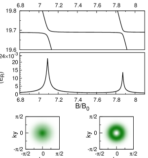
Figure 3: Anharmonic trap – dipolar resonances with $\Delta{\cal M}_{z}=-2$. Upper panel: excitation energy of the two particle system in the anharmonic trap as a function of an external magnetic field. The horizontal line at small $B$ corresponds to the $|{\rm ini}\rangle$ state with both atoms fully polarized $|3\rangle|3\rangle$. Notice two avoided crossings. Middle panel: two maxima in the self-energy curve signifying strong coupling at the resonant magnetic field. Lower panel: reduced single particle densities (in $xy$ plane) of the final states accessible via $\Delta{\cal M}_{z}=-2$ resonant dipolar processes. The densities correspond to the two resonant values of the magnetic field as indicated in the middle panel.

To construct two-body eigenstates we find numerically all $s$, $p$ and $d$ eigenstates of the anharmonic potential. Then the full two-body Hamiltonian is diagonalized in this basis. There are two states $|v_{a_{1}}\rangle$ or $|v_{a_{2}}\rangle$ which are coupled to the initial one at two different magnetic fields. The resonances are visible as avoided crossings in Fig.3. At each resonance the system is effectively a two level one.

The single particle densities of the two resonantly coupled states for $V_{0}=25E_{R}$ are presented in the lowest panel of Fig.3. Let us note, that one particle density of the $|v_{a_{2}}\rangle$ state resembles a singly quantized vortex, but does not reach the zero value at the center. In the middle panel of Fig.3 we show the self energy of the $|{\rm ini}\rangle$ state as a function of the magnetic field. The self energy reaches a maximum at every resonance.

The presented here numerical results can be understood with the help of a perturbative approach with the dipolar energy being a small parameter. The state $|{\cal L}_{2}\rangle$ can be viewed as the superposition of the two states:

$$|{\cal L}_{2}\rangle=\frac{1}{\sqrt{2}}\left(|v_{d}\rangle-|v_{p}\rangle\right),$$ (26)

where the $d$-shell state $|v_{d}\rangle$ is:

$$|v_{d}\rangle=\frac{1}{2}\left(s^{\dagger}\left(d^{\dagger}_{xx}+i\sqrt{2}d^{\dagger}_{xy}-d^{\dagger}_{yy}\right)\right)|0\rangle,$$ (27)

and the $p$-shell state $|v_{p}\rangle$ has the following form:

$$|v_{p}\rangle=\frac{1}{2\sqrt{2}}\left((p^{\dagger}_{x})^{2}+i2p^{\dagger}_{x}p^{\dagger}_{y}-(p^{\dagger}_{y})^{2}\right)|0\rangle,$$ (28)

In Eq.(27) and Eq.(28) the operators $s$, $p$ , $d$ are not the same as those in the harmonic case however we use the same notation. Now the operators create a particle in $s$ , $p$ , $d$ states of the anharmonic potential.

The two resonant states are the eigenstates of the z-component of the orbital angular momentum of two particles. $|v_{d}\rangle$ is the state with one particle in the ground and the second in the $d$-state with ${\cal L}_{z}=2$. $|v_{p}\rangle$ is the state with two particles occupying the same $p$ orbital with ${\cal L}_{z}=1$. Evidently the single particle density of the second state is typical for the singly charged vortex state in a harmonic trap.

In the harmonic trap the two states have the same energies. Their relative shift introduced by anhamonicity, $\delta E$, can be estimated using the perturbative approach with $\gamma$ being the small parameter:

$$\delta E=2\gamma\Omega_{\perp}={2\over 3}.$$ (29)

The energy of $|v_{d}\rangle$ state is smaller then the energy of $|v_{p}\rangle$ state by the $2/3$ of the recoil energy. The shift does not depend on the $V_{0}$.

These states are dressed by the contact interaction whose strength is:

$$U_{22}=\frac{g_{22}}{16\pi^{3/2}}\sqrt{\Omega_{z}}\Omega_{\perp},$$ (30)

where $g_{22}=(6g_{6}+5g_{4})/11$. The dressed eigenvectors of this effective two level system are solutions of a simple eigenvalue problem:

$$\begin{pmatrix}-\delta E&U_{22}\\ U_{22}&0\end{pmatrix}\begin{pmatrix}\alpha_{a}\\ \beta_{a}\end{pmatrix}=\varepsilon_{a}\begin{pmatrix}\alpha_{a}\\ \beta_{a}\end{pmatrix}.$$ (31)

The two eigenstates $|v_{a_{1}}\rangle=\alpha_{a}|v_{d}\rangle-\beta_{a}|v_{p}\rangle$ and $|v_{a_{2}}\rangle=\beta_{a}|v_{d}\rangle+\alpha_{a}|v_{p}\rangle$ are superpositions of the two coupled states $|v_{d}\rangle$ and $|v_{p}\rangle$.

If the contact interaction significantly exceeds the energy splitting $U_{22}>>\delta E/2$, i.e. for:

$$V_{0}>>\frac{256}{9}\frac{\pi^{3}}{(g_{22})^{2}\Omega_{z}},$$ (32)

then the harmonicity is recovered in a deep optical lattice in the strong coupling limit.

Note the crucial role of the axial trapping frequency. In a prolate geometry the harmonicity is recovered for much deeper traps than in a case of an oblate geometry. For $\Omega_{z}=16$ as used here, the anharmonicity of the optical lattices becomes negligible if $V_{0}>>29E_{R}$. In this limit the eigenvectors of the Hamiltonian are $|v_{a_{1}}\rangle\simeq(|v_{d}\rangle-|v_{p}\rangle)/\sqrt{2}$ and $|v_{a_{2}}\rangle\simeq(|v_{d}\rangle+|v_{p}\rangle)/\sqrt{2}$. Note, that the eigenstate $|v_{a_{1}}\rangle$ corresponds to relative excitations and is the same as the state reached by the dipolar interactions in the harmonic trap, $|v_{a_{1}}\rangle\simeq|{\cal L}_{2}\rangle$. The second one, $|v_{a_{2}}\rangle$, decouples from the initial $|{\rm ini}\rangle$ state as the corresponding dipolar matrix element vanishes. This states corresponds to the center of mass excitation. Obviously excitation of the center of mass is not possible in the harmonic trap by any two-body interactions. We checked that even for deep optical lattices, i.e. $V_{0}=40E_{R}$, the effect of anharmonicity cannot be neglected.

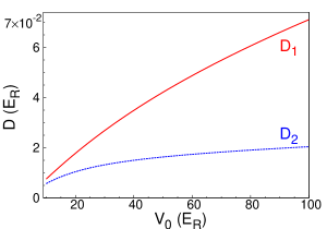
Figure 4: Dipolar matrix elments $D_{1}=|\langle v_{a_{1}}|H_{D}|{\rm ini}\rangle|$ and $D_{2}=|\langle v_{a_{2}}|H_{D}|{\rm ini}\rangle|$ for an axially symmeric anharmonic potential. With increasing barrier height the coupling to the state with no center of mass excitation dominates $D_{1}\sim\sqrt{V_{0}}$ and the harmonic limit is recovered

The way the harmonicity is recovered is quite interesting. First, the strong coupling results in a very large splitting of resonant energies with respect to the harmonic case. Separation of both resonances increases with a lattice height. Moreover the dipolar matrix element $D_{1}=\langle v_{a_{1}}|H_{D}|{\rm ini}\rangle$ grows with the barrier height $D_{1}\sim V_{0}^{1/2}$, while the coupling to the second resonant state $D_{2}=\langle v_{a_{2}}|H_{D}|{\rm ini}\rangle$ is small and independent of $V_{0}$ ($\sim\delta E$), see Fig.4. This way for very high lattices $D_{2}/D_{1}$ becomes very small and only one resonant state is resonantly coupled via the dipole-dipole intaractions.

The other extreme is shallow optical lattice. The contact interactions become negligible, $U_{22}<<\delta E/2$. The eigenstates of the interacting systems can be approximated by the $|v_{a_{1}}\rangle\simeq|v_{d}\rangle$ and $|v_{a_{2}}\rangle\simeq|v_{p}\rangle$. The one-particle density of the latter state is characteristic for a singly quantized vortex - it is therefore a perfect candidate to observe the EdH effect. The case shown in Fig.3 corresponds to a crossover situation $\delta E\sim U_{22}$.

Till now we did not take into account the spin dynamics due to the contact interaction in the final $|2\rangle|2\rangle$ spin space of the doublon. This simplification is justified if coupling due to contact interactions is ‘turned off’ by a relative light shift of energies of $m=3$ and $m=2$ states. If it is not the case then the contact interactions following the dipolar process can further transfer the doublon to $|3\rangle|1\rangle$ spin state.

Somewhat oversimplified picture of $|2\rangle|2\rangle$ to $|3\rangle|1\rangle$ coupling is based on the observation that the eigenstates $|v_{a_{1}}\rangle$ and $|v_{a_{2}}\rangle$ of the two body contact Hamiltonian have their analogons of the same eigenenergies and the same wavefunctions in $|1\rangle|3\rangle$ subspace. If so, then the state $|v_{a_{i}}\rangle|2\rangle|2\rangle$ ($i=1,2$) is coupled to $|v_{a_{i}}\rangle(|1\rangle|3\rangle+|3\rangle|1\rangle)/\sqrt{2}$ state due to the contact term $g_{22,31}\langle v_{a_{i}}|\delta({\bf r}_{1}-{\bf r}_{2})|v_{a_{i}}\rangle$. Then the form of the two-body wavefunction in $|3\rangle|1\rangle$ space is inherited from the $|2\rangle|2\rangle$ subspace.

Situation is more complicated however. The contact interactions are different in different spin subspaces. They are proportional to $g_{22}=(6g_{6}+5g_{4})/11$ or to $g_{31}=(5g_{6}+6g_{4})/11$ in $|2\rangle|2\rangle$ or in $|3\rangle|1\rangle$ spin subspace respectively. For this reason the vectors diagonalizing contact interactions in $|3\rangle|1\rangle$ space are different then $|v_{a_{1}}\rangle$ and $|v_{a_{2}}\rangle$ diagonalizing the contact interactions in the $|2\rangle|2\rangle$ space. Their eigenenergies are also different. Note however that difference in the contact interaction strength is $g_{22}-g_{31}=g_{22,31}/\sqrt{30}$, i.e. by factor $\/\sqrt{30}$ smaller than the term coupling both spin subspaces $g_{22,31}$. For this reason, the simplified discussion is not totally wrong.

Exact treatment requires taking into account two pairs of vectors from different subspaces. In order to find the states of the doublon dressed by the contact interactions one has to diagonalize the $4\times 4$ matrix in the basis of $|v_{d}\rangle$ and $|v_{p}\rangle$ states in the two involved spin subspaces. The splitting of energies of the four eigenstates is determined by the contact interactions. The eigenstates are superpositions of different spin states of the doublon. Each of them can be reached in the dipolar relaxation process if the external magnetic field is tuned to the given resonant value.

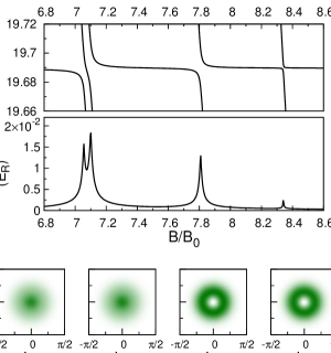
Figure 5: Anharmonic trap – dipolar resonances with $\Delta{\cal M}_{z}=-2$ when the contact interaction coupling $|2\rangle|2\rangle$ and $|3\rangle|1\rangle$ spin states is included (compare Fig.3 where this coupling was omitted). Upper panel: excitation energy of the two particle system in the anharmonic trap as a function of an external magnetic field (upper panel). The horizontal line at small $B$ corresponds to the $|{\rm ini}\rangle$ state with both atoms fully polarized $|3\rangle|3\rangle$. Notice four avoided crossings. Middle panel: four maxima in the self-energy curve signifying strong coupling at resonant magnetic field. Lower panel: reduced single particle densities (in $xy$ plane) of the final states accessible via $\Delta{\cal M}_{z}=-2$ resonant dipolar processes and the spin dependent contact interactions corresponding to the four resonant values of the magnetic fields as indicated in the middle panel.

In Fig.5 the four resonances are clearly visible for $V_{0}=25E_{R}$. The single particle densities corresponding to the every resonant state of the doublon are shown in the lowest panel. Let us observe first that the parameters we choose are in the crossover region. The anharmonic shift of energies, although does not dominate the contact interactions, is still important. The low magnetic field resonant state, in both spin subspaces, is dominated by the $d$-shell $|v_{d}\rangle$ orbital with one particle in the trap ground state (low panel of Fig.5). That is why the single particle density is large in the trap center. The higher field resonant state is dominated by the $p$-shell excitation. This is the reason of the density minimum at the center.

A small anharmonicity of the binding potential significantly modifies the spin dynamics. In the harmonic trap the two atoms oscillate between $|{\rm ini}\rangle|3\rangle|3\rangle$ and $|{\cal L}_{2}\rangle|2\rangle|2\rangle$ state at the resonant magnetic field $B_{res}$. The $|{\cal L}_{2}\rangle$ state is characterized by the orbital angular momentum ${\cal L}_{z}=2$ with no center of mass excitations. For a realistic lattice depth this single resonance splits into four resonances. The wavefunctions of the doublon are, in all four cases, eigenstates of the ${\cal L}_{z}$ component of the orbital angular momentum (with the center of mass excitation). The states are entangled. This entanglement can be usefull, particularly after applying a Stern-Gerlach magnetic field separating spatially different entangled magnetic components of the doublon.

IV.3 Single site of a square lattice

Finally we are ready to discuss a realistic situation of two atoms in a single site of the square optical lattice where both: the effect of anharmonicity and anisotropy are present simultaneously. Again, in order to find final states of the doublon which are accessible via dipolar interactions starting from the initial $|{\rm ini}\rangle|3\rangle|3\rangle$ state we have to find the eigenstates of the single particle and contact Hamiltonian $H_{0}+H_{Z}+H_{C}$. To this end we have to adjust the single particle basis to the lattice case. Instead of oscillatory wavefunctions we use the Wannier states (except of the $z$-component part which is the ground state wavefunction of the harmonic oscillator in the z-direction. To simplify a notation we omit the z-dependence of the basis wavefunction - but we keep it in our calculations). If we limit our basis to the three lowest bands in the lattice then the best approximation to the vortex state is the state created by the operator $v_{2}^{\dagger}$ as defined in Eq.(IV.1). The operators $s^{\dagger}$, $p_{x}^{\dagger}$, $p_{y}^{\dagger}$, $d_{xx}^{\dagger}$, $d_{yy}^{\dagger}$, $d_{xy}^{\dagger}$ have slightly different meaning now. They generate a particle in the Wannier states ${\cal W}_{l}(x)$ rather than in the harmonic oscillator states. For example $s^{\dagger}$ creates particle in the $\Psi_{00}={\cal W}_{0}(x){\cal W}_{0}(y)$ state, $d_{xx}^{\dagger}$ in the $\Psi_{20}={\cal W}_{2}(x){\cal W}_{0}(y)$ state, or $d_{xy}^{\dagger}$ in the $\Psi_{11}={\cal W}_{1}(x){\cal W}_{1}(y)$ state, etc.

It is convenient to rearrange the terms in the expression for the vortex state $|{\cal L}_{2}\rangle$ according to their single particle energies in the lattice, i.e:

$$|{\cal L}_{2}\rangle=|{\rm v}_{1}\rangle+|{\rm v}_{2}\rangle+|{\rm v}_{3}\rangle,$$ (33)

where:

$$|{\rm v}_{1}\rangle = \frac{1}{2\sqrt{2}}\left(s^{\dagger}\left(d_{xx}^{\dagger}-d_{yy}^{\dagger}\right)\right)|0\rangle,$$ (34)

$$|{\rm v}_{2}\rangle = -\frac{1}{4}\left(p_{x}^{\dagger}p_{x}^{\dagger}-p_{y}^{\dagger}p_{y}^{\dagger}\right)|0\rangle,$$ (35)

$$|{\rm v}_{3}\rangle = \frac{i}{2}\left(s^{\dagger}d_{xy}^{\dagger}-p_{x}^{\dagger}p_{y}^{\dagger}\right)|0\rangle.$$ (36)

The single particle contribution to the energies of these states are $E_{1}=E_{s}+E_{d}$, $E_{2}=2E_{p}$, and $E_{3}=E_{2}$ respectively, where $E_{i}^{(1D)}=\langle{\cal W}_{i}|H_{0}|{\cal W}_{i}\rangle$ is the mean energy of particle in the given Wannier state. The single particle energies of the last two states are equal because of the $Z_{2}$ symmetry of the problem. Anharmonicity is responsible for the inequality $E_{1}<E_{2}$.

The goal is to find eigenstates of the contact Hamiltonian and decompose $|{\cal L}_{2}\rangle$ state in the basis of doublon eigenstates. Note, that the two-body wavefunction $\langle{\bf r}_{1},{\bf r}_{2}|{\rm v}_{3}\rangle$ vanishes identically, if ${\bf r}_{1}={\bf r}_{2}$, so does the contact interaction in this state as well as all possible contact interactions coupling this state to the other states. The state $|{\rm v}_{3}\rangle$ is therefore the eigenstate of the two-body Hamiltonian $H_{0}+H_{Z}+H_{C}$.

On the contrary contact interactions couple the vectors $|{\rm v}_{1}\rangle$ and $|{\rm v}_{2}\rangle$. The states $|{\rm v}_{1}\rangle$ and $|{\rm v}_{2}\rangle$ are analogous to $|v_{d}\rangle$ and $|v_{p}\rangle$ states discussed in the previous section. Their two linear superpositions diagonalize the contact Hamiltonian. The two eigenvectors can be found numerically.

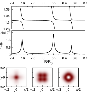
Figure 6: Single site of a square lattice – dipolar resonances with $\Delta{\cal M}_{z}=-2$ Upper panel: excitation energy of the two particle system in a single lattice site as a function of an external magnetic field. The horizontal line at small $B$corresponds to the $|{\rm ini}\rangle$ state with both atoms fully polarized $|3\rangle|3\rangle$. Notice three avoided crossing. Middle panel: three maxima in the self-energy curve signifying strong coupling at the resonant magnetic field. Lower panel: reduced single particle densities (in $xy$ plane) of the final states accessible via $\Delta{\cal M}_{z}=-2$ resonant dipolar processes corresponding to the three resonant values of the magnetic fields as indicated in the middle panel.

In the absence of coupling to the $|3\rangle|1\rangle$ subspace, there are three low energy states which can be accessed due to the dipole-dipole interactions. The three two-body eigenenergies (meassured from the energy of the initial state) are shown in Fig.6. Avoided crossings signifying dipole coupling are clearly visible. In the lower panel the single particle densities of the states coupled to the initial one are shown, while in the middle panel the self energy of the initial state is presented. The self energy depicts position, strength and width of every resonance. Note, that for axially symmetric harmonic trap, all three resonances will coincide forming ${\cal L}_{z}=2$ vortex state in the relative coordinates space of the two atoms.

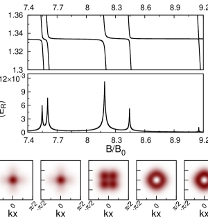
Figure 7: Single site of a square lattice – dipolar resonances with $\Delta{\cal M}_{z}=-2$ when the contact interaction coupling $|2\rangle|2\rangle$ and $|3\rangle|1\rangle$ spin states is included (compare Fig.6 where this coupling was omitted). Upper panel: the excitation energy of the two particle system in a single lattice site as a function of external magnetic field. The horizontal line at small $B$ corresponds to the $|{\rm ini}\rangle$ state with both atoms fully polarized $|3\rangle|3\rangle$. Notice five avoided crossings. Middle panel: five maxima in the self-energy curve signifying strong coupling at the resonant magnetic field. Lower panel: reduced single particle densities (in $xy$ plane) of the final states accessible via $\Delta{\cal M}_{z}=-2$ resonant dipolar processes and the spin dependent contact interactions corresponding to the five resonant values of the magnetic fields as indicated in the middle panel.

If we account for the contact interactions coupling $|{\rm v}_{1}\rangle$ and $|{\rm v}_{2}\rangle$ states in $|2\rangle|2\rangle$ spin subspace to analogous states in $|3\rangle|1\rangle$ subspace the additional channels of the spin dynamics do appear. The situation is analogous to the one discussed in the case of anharmonic trap. Again, the $4\times 4$ eigenvalue problem leads to four different eigenvectors with entangled spin and spatial wavefunctions. Together with $|{\rm v}_{3}\rangle$ state there are five low energy dipolar states resonantly coupled to the initial one in the single site of the optical lattice. The state $|{\rm v}_{3}\rangle$ is not shifted by contact interactions, ‘lives’ entirely in the $|2\rangle|2\rangle$ spin subspace. All the resonances obtained by numerical diagonalization of the full Hamiltonian in the Wannier basis are visible in Fig.7. The single particle densities of the states accessible by the dipole-dipole interactions (summed over final spin projection) are shown in the lower panel.

V Comparison with the experiment

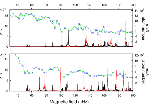
Figure 8: Comparison with the experiment: The self energy as a function of the Larmor frequency for the rectangular lattice of anisotropic sites - black lines. The assumed here lattice potential is separable and in every spatial direction has a form of a $`\sin^{2}$’ function. Quadratic terms in the expantion of the potential correspond to the following harmonic frequencies: $\omega_{x}/2\pi=160$kHz, $\omega_{y}/2\pi=60$kHz and $\omega_{z}/2\pi=90$kHz. Two orthogonal orientations of the magnetic field in the horizonatal plane, similarly as in the experiment, are considered: $y$ direction – upper panel, $x$ direction – lower panel. Occupation of the initial $m=3$ state as measured experimentaly in Tolra_rezonanse is shown for comaprison – circles. The occupation should exhibit a local minimum at every resonance. The red dashed line correspods to the self energy obtained from the harmonic approximation, $\omega_{x}/2\pi=170$kHz, $\omega_{y}/2\pi=55$kHz and $\omega_{z}/2\pi=100$kHz, without any two-body interactions as used in Tolra_rezonanse . Trap frequencies

Resonant demagnetization of initially polarized ${}^{52}Cr$ atoms in $|m_{S}=3\rangle$ state in optical lattice at ultra low magnetic fields has been observed recently Tolra_rezonanse . This process is possible because of the dipole-dipole interactions. Due to a geometrical configuration of laser beams the lattice has quite complicated geometry and results presented in the previous sections do not directly apply to the experiment.

In this section we present quite realistic calculations for parameters of the experiment Tolra_rezonanse . The lattice barrier in the horizontal plane is sufficiently high, $V_{0}=25E_{R}$, therefore the experimental system is in the Mott insulating state with two particle per site. We neglect tunneling and possible lattice inhomogeneities so we do not consider situations with three or more atoms per site.

In the horizontal plane the main axes of a single site are tilted with respect to the lines connecting the lattice minima. The single site is anisotropic. In the harmonic approximation frequencies of a site potential are $\omega_{x}/2\pi=170(10)$kHz, $\omega_{y}/2\pi=55(5)$kHz and $\omega_{z}/2\pi=100(10)$kHz. The realistic potential is non separable and cannot be approximated by the sum of ‘sine square’ functions as studied here. In particular the expansion of the potential around the minimum gives, in addition to quadratic, also the third order terms. They are not present in the expansion of the ‘sin square’ potential. Exact treatment requires construction of realistic Wannier functions. Such an approach goes beyond the scope of this paper. Instead we will fit theoretical results for the 3D lattice potential of the form:

$$V(x,y,z)=V_{0}\big{[}\sin^{2}(k_{x}x)+\sin^{2}(k_{y}y)\big{]}+V_{z}\sin^{2}(k_{z}z),$$ (37)

to the experimental data. In Eq.(37) $V_{0}=25E_{R}$ and $k_{z}=1$. The remaining parameters $k_{x}$, $k_{y}$, and $V_{z}$ are choosen to get the harmonic frequencies $\omega_{x}=2k_{x}\sqrt{V_{0}}$, $\omega_{y}=2k_{y}\sqrt{V_{0}}$, $\omega_{z}=2\sqrt{V_{z}}$, in an agreement with the experimental arrangement.

The range of magnetic fields studied experimentally corresponds to the Larmor frequency $\hbar\omega_{L}=g\mu_{B}B<\hbar 2\pi\times 200$kHz. In this region there is a number of excited orbital states which are accessible via dipole-dipole interactions. The selection rules following from the particular form of the dipole-dipole interactions give limitations on the states. They can be labeled by a number of excitation quanta of vibrational motion of the doublon $(N_{x},N_{y},N_{z})$. For the magnetic field directed along the z-axis the selection rules are the following: i) If $\Delta{\cal M}=-1$ then the quantum numbers $N_{x}$ and $N_{z}$ are odd but $N_{y}$ is even or $N_{y}$ and $N_{z}$ are odd while $N_{x}$ is even. ii) For processes with $\Delta{\cal M}=-2$, the final states must be characterized by even values of the sum $N_{x}+N_{y}$ and even values of $N_{z}$. For the range of magnetic field studied experimentally doublon states of energies up to $E_{fin}=(N_{x}\omega_{x}+N_{y}\omega_{y}+N_{z}\omega_{z})E_{R}<\hbar(2\pi\times 400)$kHz can be populated. This condition combined with the selection rules gives 10 resonantly coupled states for orientation of the external magnetic field parallel to the x-axis and 8 states for the field orientation along the y-axis. Detailed specification of the final states is given in Tolra_rezonanse .

In the harmonic trap only the relative orbital motion of two interacting atoms can be excited therefore the final state is unique. This is no longer true in realistic anharmonic potentials. The quantum numbers $(N_{x},N_{y},N_{z})$ define an energy band. The excitation energy is shared by two atoms, i.e. $N_{i}=n_{i}+n^{\prime}_{i}$, ($i=x,y,z$), where $n_{i}$ and $n^{\prime}_{i}$ are excitation quanta of individual atoms. Within the given energy band there are many two particle states (obeying the bosonic symmetry) which can be coupled by the dipole-dipole interactions to the initial state. To find the positions of dipolar resonances as well as their ’strength’ we diagonalize the full Hamiltonian of the two particle system in the basis of two-particle states which includes the initial state as well as all the states belonging to all the energy bands within interesting energy range. We include all inter- and intra-band contact interactions between particles in the basis states. The intra-band interactions are not negligible as the smallest band spacing $\omega_{y}=2\pi\times 55$kHz is not much larger than the characteristic contact interactions $\sim 2\pi\times 10$kHz. We include $|2\rangle|2\rangle$ as well as $1/\sqrt{2}(|3\rangle|1\rangle+|1\rangle|3\rangle$ spin states for excited system. This way we take into account a possible transfer of atoms from the $|2\rangle|2\rangle$ to $|3\rangle|1\rangle$ spin space due to the spin changing contact interactions.

The results for two different orientations of the magnetic field are presented in Fig.8. To compare them with experimental data of Tolra_rezonanse we plot the self energy as a value of magnetic field (Larmor frequency). The self energy displays a sharp maximum (black lines) at every resonant value of the magnetic field. The points correspond to the experimental data as copied from the paper Tolra_rezonanse (Fig.2) and indicate the number of atoms left in the initial $m=3$ state. This quantity should be small at the resonance, i.e. minima in the experimental curve ought to correspond to maxima of the self energy. For comparison we show the self energy in the harmonic approximation with all contact interaction set to zero as shown in Fig.2 in Tolra_rezonanse – dashed (red) line.

The first observation is that the very fine structures predicted theoretically are significantly narrower than resonant features observed. They are simply not resolved in the experiment. The reasons for this were discussed in the experimental paper and are attributed mainly to the increasing band-width for higher energy lattices bands but also to the magnetic field and lattice depth fluctuations which are broadening the resonances, at the 10 kHz level. The extremely precise control of magnetic field, probably beyond the level of experimental reach is required.

The second observation is that the structure of resonances is very reach. This fact is obvious on the basis of results presented here: degeneracy of every energy shell is removed because of anharmonicity and anisotropy and all the states become accessible via the dipole-dipole interactions.

Finally because of anharmonicity and the contact interactions the positions of the resonances are shifted towards lower magnetic fields. Note that both above mentioned effects act (mainly) in the same direction. The energy shift can be as large as $2\pi\times 10$kHz for the states excited to the high Wannier bands.

The anharmonicity and anisotropy of the lattice does not affect significantly the widths of the resonances. Their main effect is to split the every resonant peak into a reach fine structure. The width of an individual fine resonant feature is smaller than the width predicted in the harmonic approximation, but its magnitude remains at the same level, i.e. $\sim 10\mu$G. It is probably not possible, to resolve these fine structures experimentally. On the other hand, splitting of the singe resonant peak results in an overall broadening of the entire structure composed of several fine features. The broadening due to this splitting is given by the contact interactions strength and corresponds to the magnetic fields $\sim 1-10$mG. A precise control of the magnetic field at this level is quite realistic. The widths of observed in Tolra_rezonanse resonant features ($\sim 10$kHz) correspond to the above estimation and, according to our analysis, can be attributed to the effects of anharmonicity and anisotropy of the binding potential.

The resonant character of the process is visible in a region of low Larmor frequencies only. At the first glance there are only few distinct experimental resonances in the region of small Larmor frequencies. By choosing the following values of the site frequencies: $\omega_{x}/2\pi=160$kHz, $\omega_{y}/2\pi=60$kHz, $\omega_{z}/2\pi=110$kHz, we can reproduce reasonably well the positions of the three first minima for the case with the magnetic field directed along the x-axis. The similar agreement we get for the orientation of the magnetic field along the y-axis. In the region of large $\omega_{L}$ where highly excited states become occupied, resonances are relatively close to each other and their number increases. Different resonant structure start to overlap. Therefore at higher magnetic fields, due to the fine splitting of neighboring resonances the resonant character of the process should be lost. This is clearly seen in the experimental data for large $\omega_{L}$.

The fitted frequencies have values within the given range of experimental uncertainties however they are different than the harmonic frequencies used in the experimental paper to get the red dashed lines in Fig.8. The positions of experimentally resolved resonances can be reproduced theoretically regardless whether anharmonicity and anisotropy of the lattice potential are taken into account or not. Small uncertaintities of the lattice parameters, as well as their fluctuations, give sufficient freedom to allow for fitting positions of the resonances using both a simple harmonic theory without any two-body interactions as well as quite advanced approach accounting for all interactions and anharmonicity and anisotropy of the lattice sites. However, the overall widths of the entire fine structures cannot be reproduced in the harmonic approximation.

VI Final Remarks

We have shown that the dipole-dipole interactions are very effective probe of the two-body states of Chromium atoms in the external trapping potential. They are very sensitive to anharmonicity and symmetry of the single site. The anharmonicity of the single trap becomes very important in particular when higher Wannier states with non vanishing angular momentum are concerned. The contact interactions between the degenerate states in the site lift the degeneracy and introduce a fine structure of the energy spectrum of the system. Spectroscopy of this fine structure can be done with the help of the dipolar resonances. Observation of spin dynamics driven by the contact interactions is a precise method of determination of contact interaction for both Fermi and Bose atoms Bloch ; Sengstock . We show that spin dynamics due to dipolar interactions at the resonant magnetic field is yet another perfect tool for precise determination of the scattering lengths of involved atoms. This can be very important for measurement of the various scattering length for dipolar elements such as Dysprosium or Erbium Lev ; Ferlaino . Generalization of the approach presented here to more atoms per site or Fermi species is straightforward.

- (1) Y. Kawaguchi and M. Ueda, Phys. Rep. 520, 253 (2012).
- (2) O. W. Richardson, A mechanical effect accompanying magnetization, Physical Review (Series I), Vol. 26, Issue 3, pp. 248 96253 (1908).
- (3) A. Einstein, W. J. de Haas, Experimenteller Nachweis der Ampereschen Molekularst F6rme, Deutsche Physikalische Gesellschaft, Verhandlungen 17, pp. 152 96170 (1915).
- (4) A. Einstein, W. J. de Haas, Experimental proof of the existence of Ampe‘re’s molecular currents (in English), Koninklijke Akademie van Wetenschappen te Amsterdam, Proceedings, 18 I, pp. 696 96711 (1915).
- (5) Y. Kawaguchi, H. Saito, and M. Ueda, Phys. Rev. Lett. 96, 080405 (2006).
- (6) L. Santos and T. Pfau, Phys. Rev. Lett. 96, 190404 (2006).
- (7) K. Gawryluk, M. Brewczyk, K. Bongs, and M. Gajda, Phys. Rev. Lett. 99, 130401 (2007).
- (8) T. Świsłocki, T. Sowiński, J. Pietraszewicz, M. Brewczyk, M. Lewenstein, J. Zakrzewski, M. Gajda, Phys. Rev. A 83, 063617 (2011)
- (9) B. Pasquiou, E. Maréchal, G. Bismut, P. Pedri, L. Vernac, O. Gorceix, and B. Laburthe-Tolra, Phys. Rev. Lett. 106, 255303 (2011)
- (10) K. Gawryluk, K. Bongs, M. Brewczyk, Phys. Rev. Lett. 106, 140403 (2011)
- (11) J. Pietraszewicz, T. Sowiński, M. Brewczyk, J. Zakrzewski, M. Lewenstein, M. Gajda, Phys. Rev. A 85, 053638 (2012)
- (12) A. de Paz, A. Chotia, E. Maréchal, P. Pedri, L. Vernac, O. Gorceix,B. Laburthe-Tolra, Phys. Rev. A 87, 051609(R) (2013).
- (13) X. Li, Z. Zhang, W. V. Liu, Phys. Rev. Lett. 108, 175302 (2012)
- (14) B. Sun and L. You, Phys. Rev. Lett. 99, 150402 (2007).
- (15) A. Collin, J. Larson, and J.-P. Martikainen, Phys. Rev. A 81, 023605 (2010)
- (16) F. Pinheiro, J.-P. Martikainen, J. Larson, Phys. Rev. A 85, 033638 (2012)
- (17) A. Widera, F. Garbier, S. Folling, T. Gericke, O. Mandel, I. Bloch, New J. Phys. 8, 152 (2006).
- (18) J. S. Krauser, J. Heinze, N. Fläschner, S. Götze, Ch. Becker, K. Sengstock, Nature Phys.8, 813 (2012)
- (19) M. Lu, N. Q. Burdick, S. H. Youn, B. L. Lev, Phys. Rev. Lett. 107, 190401 (2011)
- (20) K. Aikawa, A. Frisch, M. Mark, S. Baier, A. Rietzler, R. Grimm, F. Ferlaino, Phys. Rev. Lett. 108, 210401 (2012)