Biases in physical parameter estimates through differential lensing magnification

Abstract

We study the lensing magnification effect on background galaxies. Differential magnification due to different magnifications of different source regions of a galaxy will change the lensed composite spectra. The derived properties of the background galaxies are therefore biased. For simplicity, we model galaxies as a superposition of an axis-symmetric bulge and a face-on disk in order to study the differential magnification effect on the composite spectra. We find that some properties derived from the spectra (e.g., velocity dispersion, star formation rate and metallicity) are modified. Depending on the relative positions of the source and the lens, the inferred results can be either over- or under-estimates of the true values. In general, for an extended source at strong lensing regions with high magnifications, the inferred physical parameters (e.g. metallicity) can be strongly biased. Therefore detailed lens modelling is necessary to obtain the true properties of the lensed galaxies.

1. Introduction

The properties of high redshift objects, mostly galaxies, provide important information on the early evolution of galaxies and the role they played in the cosmic reionization (e.g. Loeb, 2010; Fan, 2012). Observations of the high redshift galaxies are challenging due to large distances and faint magnitudes. With the growing power of telescopes, the number of high redshift galaxies found is increasing rapidly, either by deep imaging or the color selection (the $V$-band, $r$-band “dropout” technique) (e.g. Stanway et al., 2004; Hildebrandt et al., 2009). Moreover, the $Y-$band and $J-$band dropouts can potentially detect objects at redshift $z\sim 8$ (e.g. Yan et al., 2012). Galaxy clusters, as nature telescopes can enhance the ability to detect high redshift galaxies (Soucail, 1990). The method has been implemented to study galaxies over a wide range of redshifts (e.g. Ellis et al., 2001; Bradač et al., 2009; Hall et al., 2012) as well as Ly$\alpha$ spheres (Li et al., 2007). It has been shown that the search for the high-$z$ galaxies ($z>7$) in a lensing field is more efficient than that in blank fields, and the maximum efficiency is reached for lens clusters at $z\sim 0.1-0.3$ (Maizy et al., 2010).

Gravitational lensing provides a direct way for studying the mass distribution of the large scale structures in the universe as well as galactic- and cluster-sized halos (e.g. Bartelmann & Schneider, 2001; Treu, 2010). On the other hand, the light from distant galaxies can be magnified by several orders of magnitude by the gravitational potential well of massive galaxy clusters. The effective solid angle of the survey volume decreases in the same way. However, since the luminosity function is exponential at the bright end, the magnification significantly increases the number counts of luminous galaxies (e.g. Lima et al., 2010; Er et al., 2013). In addition, the lensing magnification improves the spatial resolution of distant galaxies (e.g. Stark et al., 2008; McKean et al., 2011; Fan et al., 2012; Jones et al., 2013). For multiply-imaged systems, the positions and magnitudes of the images depend on several factors, e.g., lens and source redshifts, lens mass profiles (including substructures, e.g. Mao & Schneider 1998) and intrinsic properties of the background sources. Thus gravitational lensing provides us with more information for studying both lens galaxies and background sources.

Lensing magnification itself is achromatic. However, magnification varies with the position of the source. The spatial profiles at different wavelengths may not be the same. Thus a source at different wavelengths may be magnified differently (Blandford & Narayan, 1992). It has been noticed that differential magnification can bias the derived results using the spectral energy distribution (SED) of lensed sources (e.g. Blain, 1999; Pontoppidan & Wiklind, 2001), or using the ratio of spectral lines (e.g. Downes et al., 1995). Hezaveh et al. (2012) modelled their sources with two components (a compact and a diffuse one) and showed that the compact one will usually be magnified by a larger factor than the diffuse one in strong lensing.

In this paper, we will study the bias in the derived spectral physical parameters due to differential magnification. We model the background galaxy as a sum of a bulge and a disk with different sizes and spectra. Using ray-tracing simulations, the lensing magnifications of different regions are calculated and applied to obtain the composite observed spectrum. We start with a discussion of the basic formalism in section 2, present our model and magnification effects in section 3, and then discuss our results in section 4. The cosmology adopted here is a $\Lambda$CDM model with parameters based on Kilbinger et al. (2012): $\Omega_{\Lambda}=0.718$, $\Omega_{\rm m}=0.286$, $\sigma_{8}=0.804$, a Hubble constant $H_{0}=100h$ km s^-1 Mpc^-1 with $h=0.693$.

2. Lensing magnification

The fundamentals of gravitational lensing can be found in Bartelmann & Schneider (2001). The thin-lens approximation is adopted in this paper, implying that the lens mass distribution can be projected onto the lens plane perpendicular to the line of sight. We denote angular coordinates on the lens plane as $\theta$, and those on the source plane as $\beta$. The lens equation can be written as

$$\mbox{\boldmath$\beta$}=\mbox{\boldmath$\theta$}-{D_{\rm ds}\over D_{\rm s}}\hat{\alpha}(\mbox{\boldmath$\theta$})=\mbox{\boldmath$\theta$}-\mbox{\boldmath$\alpha(\theta)$},$$ (1)

where $D_{\rm ds}$ and $D_{\rm s}$ are the angular diameter distances from the lens to the source and from the observer to the source respectively. The deflection angle $\alpha$ can be calculated from the lens model.

We denote the brightness distribution of the source by $I^{s}(\mbox{\boldmath$\beta$})$. Since lensing conserves the surface brightness, the brightness distribution of the image is thus $I(\mbox{\boldmath$\theta$})=I^{s}(\mbox{\boldmath$\beta$}(\mbox{\boldmath$\theta$}))$. The total flux of the source and image are

$$S_{0}=\int\mathrm{d}^{2}\beta\;I^{s}(\mbox{\boldmath$\beta$}),\qquad S=\int\mathrm{d}^{2}\theta\;I(\mbox{\boldmath$\theta$}),$$ (2)

respectively. The magnification is defined as $\mu\equiv S/S_{0}$.

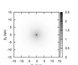
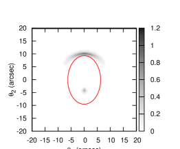
Figure 1.— The simulated image of a background source (left) and the lensed (right) images. Notice that the scales and units of the two panels are different. In the right panel, the lens is at the origin of the map with $\theta_{\rm E}=7.8$ arcsec ($\sim 15$kpc). The solid line is the critical curve of the lens. The lens and source are at redshift 0.1 and 2.0 respectively.

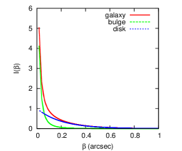
Figure 2.— The left panel shows the surface intensity profile of the source galaxy: an axis-symmetric bulge, a face-on disk component and the sum. The right panel shows the velocity dispersion variation as a function of radius.

3. Lensing effects on the spectroscopic properties of background sources

Lensing magnification varies with the relative positions of the lens and source, especially when the source is close to the caustics. For extended galaxies, different components differ in intrinsic sizes, thus their magnifications will be different. Therefore the observed spectrum of the background galaxy is changed by lensing. The estimation of galaxy properties differs from its intrinsic ones, like velocity dispersion ($\sigma_{*}$), star formation rate (SFR) and metallicity of galaxies ($Z$). In Hezaveh et al. (2012), the galaxy is modelled as the sum of an extended component and an inner core. The total flux is the sum of the two components and the total magnification is their weighted average. A similar approach will be adopted here. In reality, galaxies are structurally complicated, e.g. they host some clumpy star formation regions. Moreover, their morphology may not be regular, especially during the early stage of galaxy formation. The simple model here is for illustration purposes.

3.1. Light profile of the background galaxy

The luminosity profiles of the bulge and the disk are described as follows:

$$I(R) = I_{e}\,{\rm exp}\{-7.67\left[\left(R/R_{e}\right)^{1/4}-1\right]\},$$ (3)

$$I(R) = I_{d}\,{\rm exp}\left(-R/R_{d}\right),$$ (4)

where $I_{e}$ is the surface brightness at the bulge effective radius $R_{e}$, $I_{d}$ is the central surface brightness and $R_{d}$ is the scale length of the exponential disk. The bulge to total ratio is (Binney & Tremaine, 1987)

$$B/T={R_{e}^{2}I_{e}\over R_{e}^{2}I_{e}+0.28R_{d}^{2}I_{d}}.$$ (5)

We use $I_{d}=1.0$ and $I_{e}=0.44$ (the unit is arbitrary here, since we only need the luminosity ratio between the bulge and the disk). With a small bulge assumption in this study ($B/T=0.2$) (Lackner & Gunn, 2012), we take $R_{e}=0.7$ kpc and $R_{d}=1.7$ kpc, corresponding to $0.08$ and $0.2$ arcsec at redshift $z_{s}=2$ respectively. For simplicity, we assume an axis-symmetric bulge and a face-on disk (see the left panel of Fig. 1).

For convenience, we will use the angular separation in the rest of this paper ($1$ arcsec equals to $8.7$ kpc in the source plane $z_{s}=2$, and $1.9$ kpc in the lens plane $z_{d}=0.1$). The velocity dispersion is estimated from the surface brightness using the isothermal sheet. Further approximation, assuming a uniform disc scale height, the velocity dispersion of the source as a function of radii is given by $\sigma_{*}(\theta)\propto\sqrt{I(\theta)}$ (Binney & Tremaine, 1987, Chapter 4.4), and we set the central value as $218\,{\rm km\,s^{-1}}$ (see the right panel of Fig. 2).

The stellar velocity dispersion and the metallicity of source galaxy relies on stellar continuum, while the star formation rate (SFR) can be estimated from the [O ii] emission lines. Hence we simulate the spectra of bulge and disk by combining the emission-line spectra and the stellar continuum. For stellar continuum, four artificial stellar populations are used to generate the spectra (Bruzual & Charlot, 2003). The weight of each stellar population is set to be equal ($1/4$). Due to the metallicity gradient of galaxies (e.g. Rolleston et al., 2000), the metallicity of the bulge is set to be larger than that of the disk region (see Table 1 for more details on the stellar populations of the bulge and disk).

The emission-line spectra of the bulge and disk are also simulated separately. For the bulge there are two components: a narrow-line region (NLR) of the central active galactic nucleus (AGN) and a starburst in the bulge. For the disk there is only a starburst component. In order to study the stellar continuum, we can only take into account the emission of a type II AGN by assuming that the emissions from the accretion disk and the broad line region are obscured by the torus. The type II AGN emission-line spectrum is taken from Reyes et al. (2008). The starburst emission-line spectra are taken from SDSS DR7 with the selection criteria of [OIII]/$H{\beta}\sim 0.35$ and [NII]/$H{\alpha}\sim-1.0$, which is appropriate for the star-forming gas rich galaxies at redshift $2$. The SFRs of the bulge and disk, which are estimated by using [O ii] luminosities, are set to be proportional to the surface brightness.

Table 1Stellar populations used for the bulge and disk

Name	Age	Metallicity $Z/Z_{\odot}$
Bulge
age116$\_$m42	1.0152E+08	0.2
age070$\_$m62	1.0000E+07	1.0
age135$\_$m62	9.0479E+08	1.0
age150$\_$m72	2.5000E+09	2.25
Disk
age055$\_$m42	5.0100E+06	0.2
age070$\_$m42	1.0000E+07	0.2
age139$\_$m42	1.4340E+09	0.2
age116$\_$m62	1.0152E+08	1.0

With the chosen spectra and luminosity profiles of the bulge and the disk, the lensed spectrum of the background galaxy can be obtained after knowing the mean magnification of each part of the source:

$$F(\nu,\mbox{\boldmath$\theta$})=\mu_{b}F_{b}(\nu,\mbox{\boldmath$\theta$})+\mu_{d}F_{d}(\nu,\mbox{\boldmath$\theta$}).$$ (6)

where $\mu_{b}$ and $\mu_{d}$ are the magnifications of the bulge region ($<0.1$ arcsec) and the disk region, which can be calculated from the lensing model.

3.2. Lens modelling

In order to study the differential magnification effect on the spectrum of background sources, we perform ray-tracing simulations. For simplicity, we model our lens as a singular isothermal ellipsoid with a velocity dispersion of $770$ km/s ($M_{200}\approx 1\times 10^{14}h^{-1}M_{\odot}$) and ellipticity $\epsilon=0.2$. The lens is placed at redshift $z_{d}=0.1$, which gives an Einstein radius $\theta_{\rm E}=7.8$  arcsec. We map a grid of pixels from the lens plane to the source plane using the lens equation to obtain the surface brightness distribution of the image. From this distribution, the total flux of the image is obtained using Eq. 2. We will calculate the magnifications separately for the inner region, $\mu_{b}$ ($<0.1$ arcsec), and for the outer region ($\mu_{d}$).

The magnification ratio between the bulge and the disk strongly depends on the relative position of the source and lens, and the intrinsic size of source galaxies. In the left panel of Fig. 3, one can see that when the bulge of the source galaxy is close to the caustics, the magnification differences in the bulge and the disk are significantly larger. An interesting point is when the disk is closer to the caustics than the bulge, the ratio becomes smaller than $1$ ($\mu_{d}>\mu_{b}$). When the bulge crosses the caustics, the reverse occurs ($\mu_{b}>\mu_{d}$). As a consequence, a slight shift of the source position (or a change of the lens model) may cause a significantly different magnification ratio. One can also see that the region where the differential magnification is strong, the absolute magnification is also high (e.g. $\mu>5$, right panel of Fig. 3).

We first place the source at $\beta=(0,3)$ arcsec on the source plane (and study another position $(0.3,2.5)$ in the end). Two images are generated by lensing (see the right panel of Fig. 1). We only study the primary image in this paper, since it is more luminous and easier to detect. The mean magnification of the bulge (disk) region is $\mu_{b}=15$ ($\mu_{d}=10$).

We simulate the velocity dispersion $\sigma_{*}$ detected by different sizes of fibers. The centre of the fiber is aligned with the centre of the lensed source. The mean velocity dispersion is weighted by luminosity. In Fig. 4, the solid and dashed lines represent the $\sigma_{*}(\theta)$ after and before lensing respectively. When the fiber size becomes very small, the measured velocity dispersion approaches the intrinsic ones; in the other cases, the measurements of the lensed galaxy are larger than the initial ones for $\beta=(0,3)$.

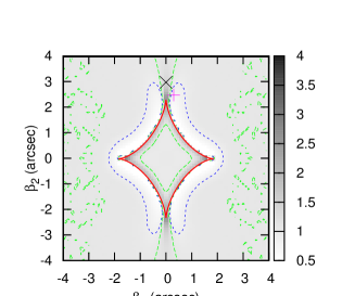
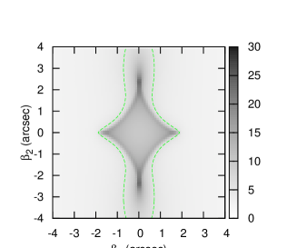
Figure 3.— $Left:$ The ratio of $\mu_{b}/\mu_{d}$ on the source plane, given on linear grey scale and contours. The blue dashed lines enclose the region where $\mu_{b}/\mu_{d}<0.85$. The green lines enclose the dark region where the ratio is greater than $1$. The red solid line is the caustics. The cross and plus represent the positions of our mock source galaxies. $Right:$ The mean magnification of the whole galaxy on the source plane. The green dashed line encloses the region where $|\mu|>5$.

Figure 4.— The luminosity-weighted mean velocity dispersion as a function of the fiber size.

3.3. Results from spectral analysis

The $\sigma_{*}$, SFR and metallicity ($Z$) variation of the source and the lensed galaxy can be obtained through the analysis of the composite spectra. According to the source model and the parameters listed in Table 2, we can fit the galactic continuum using STARLIGHT (Cid Fernandes et al., 2005). This code employs 45 stellar population templates which are composed of 3 metallicities and 15 ages (Bruzual & Charlot, 2003). The differences between the spectra of the lensed image and the initial galaxy are listed in Table 2. The velocity dispersion of the lensed image is higher in the case of $\mu_{b}$/$\mu_{d}=15/10$, since the velocity dispersion of the bulge is larger than the disk. In order to get a reliable result, we fit the spectra by using the direct pixel fitting method (Greene & Ho, 2006; Ho et al., 2009; Ge et al., 2012), and obtain the same results.

With the continuum subtracted, we can obtain the emission-line only spectra. The SFR is estimated by fitting [OII]$\lambda$3727. Here the SFR is normalized to $10M_{\odot}{\rm yr}^{-1}$ (e.g. Santini et al., 2009). The SFR derived from the lensed image is enhanced by about $11$ times in the case of $\mu_{b}$/$\mu_{d}=15/10$. After correcting by the mean magnification of the whole galaxy ($\mu=12.7$), the SFR result is smaller than the true value by $\sim 10\%$.

The metallicity of the whole galaxy is again obtained from the STARLIGHT, $Z=\Sigma x_{j}\times Z_{j}$, where $x_{j}$ is the weight of the $j$-th stellar population, and $Z_{j}$ is its metallicity. The result from the lensed image is significantly larger than the initial one. The reason is that both the metallicity and the magnification of the bulge are higher than those of the disk, and the weight of the bulge is enlarged by lensing.

To see the sensitivity of the results to the source position, we place the source at a different location $(0.3,2.5)$. The results are given in the column ‘lensed 2’ in Table 2. The magnification ratio is different from the first case: $\mu_{b}/\mu_{d}=7/10$. In this case, the contribution of the bulge to the total lensed spectrum is suppressed, which leads to a smaller $\sigma_{*}$ and metallicity while the SFR is overestimated.

When we observe the lensed galaxy with fibers, the light may actually come from different parts of the bulge and the disk, which makes the measurement of velocity dispersion, SFR and metallicity of the source more complicated. We perform simulations with a fiber size of $3$ arcsec diameter. The centre of the lensed image is identified as the brightest position of the image. The results are given in the bottom part of Table 2. For both source positions, similar biases are obtained.

Table 2Results of differential magnification

Parameters	Bulge	Disk	lensed $1$	lensed $2$	Source
total flux
$\mu$	15(7)	10(10)	15+10	7+10	1+1
luminosity	1	4	58	50	5
$\sigma_{*}$(km/s)	131	48	67	58	59
SFR (10$h^{-1}M_{\odot}$/yr)	2	8	113(8.9)	93(11)	10
metallicity $Z/Z_{\odot}$	0.95	0.4	0.59	0.47	0.51
flux within 3 arcsec diameter fiber
$\mu$	15(6.7)	13.5(6.6)	15+13.5	6.7+6.6	1+1
luminosity	1	0.67	19	11	1.67
$\sigma_{*}$(km/s)	164(134)	53(52)	118	76	110 (74)
SFR (10$h^{-1}M_{\odot}$/yr)	6	4	144(9.6)	67(10)	10
metallicity $Z/Z_{\odot}$	0.95	0.4	0.8	0.58	0.61

Note. — The column ‘lensed 1’ represents the lensed results for the source position $(0,3)$ (black cross in Fig. 3), while the column ‘lensed 2’ represents the results for the source position $(0.3,2.5)$ (purple plus in Fig. 3). $\sigma_{*}$ is the velocity dispersion estimated using the method in Ge et al. (2012). The SFR in brackets is corrected by the mean magnification of the whole lensed galaxy.

4. Summary and discussion

In this paper, we have studied the differential magnification effect on the spectrum of a lensed background galaxy. Two components (a bulge and a disk) with different luminosity profiles and spectra are used to model the background galaxy. Ray-tracing simulations are employed to calculate the lensing magnification. We find that the derived properties of the lensed galaxy are changed, e.g. SFR, metallicity and velocity dispersion. Velocity dispersion and metallicity can either increase or decrease, depending on the relative position of the source and the lens. The SFR is strongly enhanced but can be corrected by dividing the mean magnification. However, a slight bias of SFR still remains after correction. Not surprisingly, the differential magnification will be strong when the source is close to the caustics, and the absolute value of the magnification is also high (e.g. $|\mu|>5$). In this case, a slight shift of the source position will cause a dramatic change in the derived results. Therefore, one needs to take into account the differential magnification effect for highly magnified extended sources.

Because of observational limitations, the black hole vs. velocity dispersion ($M_{\rm BH}-\sigma_{*}$) relation at high redshift (e.g. Tremaine et al., 2002) is uncertain. Gravitational lensing boosts our chances of studying black holes at high redshift. However, we found that the measured $\sigma_{*}$ may be an unreliable indicator of the black hole mass. In practice, for very high-redshift galaxies, it is easier to observe with slits than fibres since the background subtraction is more reliable. To avoid extra bias entering the results, one needs to consider carefully the region of the background galaxy covered when taking a spectrum.

Our study is simplistic in several ways. For example, source galaxies may be irregular, lacking regular bulge and disk components. Additionally, high redshift galaxies can be complicated, e.g. they may have clumpy star forming regions with different spectra (Genzel et al., 2008; Jones et al., 2013). This will mislead the calculation of derived physical properties. Moreover, lens clusters are also complicated. The magnification map is strongly affected by the shape and mass profile (including substructures) of the lens. Therefore accurate lens modelling is necessary when deriving the properties of lensed galaxies.

On the other hand, multiple images can provide more constraints on both the lens and source. With Integral Field Unit (IFU) spectra for different components of the multiple images at high redshift, we can study the lens mass distribution and the intrinsic properties of background galaxies in greater detail. With iterative modelling of the lens and source, a relatively precise source image can be reconstructed. The bias due to differential magnification can be strongly suppressed.

Current telescopes, such as the Hubble Space Telescope (HST) or the Keck telescope can already study differential magnifications. The next-generation telescopes with adaptive optics, such as the Thirty Meter Telescope and the E-ELT, will allow even more accurate studies of dynamics in high redshift galaxies.

5. Acknowledgments

We thank Richard Long, Tucker Jones, and the referee for useful comments on the draft. XE is supported by NSFC grant No.11203029. SM is supported by the Chinese Academy of Sciences and the National Astronomical Observatories of China.

References

- Bartelmann & Schneider (2001) Bartelmann, M., & Schneider, P. 2001, Phys. Rep., 340, 291
- Binney & Tremaine (1987) Binney, J., & Tremaine, S. 1987, Galactic dynamics, Princeton University Press, Princeton, NJ
- Blain (1999) Blain, A. W. 1999, MNRAS, 304, 669
- Blandford & Narayan (1992) Blandford, R. D., & Narayan, R. 1992, ARA&A, 30, 311
- Bradač et al. (2009) Bradač, M., et al. 2009, ApJ, 706, 1201
- Bruzual & Charlot (2003) Bruzual, G., & Charlot, S. 2003, MNRAS, 344, 1000
- Cid Fernandes et al. (2005) Cid Fernandes, R., Mateus, A., Sodré, L., Stasińska, G., & Gomes, J. M. 2005, MNRAS, 358, 363
- Downes et al. (1995) Downes, D., Solomon, P. M., & Radford, S. J. E. 1995, ApJ, 453, L65
- Ellis et al. (2001) Ellis, R., Santos, M. R., Kneib, J.-P., & Kuijken, K. 2001, ApJ, 560, L119
- Er et al. (2013) Er, X., Li, G., Mao, S., & Cao, L. 2013, MNRAS, 430, 1423
- Fan et al. (2012) Fan, L., Chen, Y., Er, X., Li, J., Lin, L., & Kong, X. 2012, ArXiv 1212.6700
- Fan (2012) Fan, X. 2012, Research in Astronomy and Astrophysics, 12, 865
- Ge et al. (2012) Ge, J.-Q., Hu, C., Wang, J.-M., Bai, J.-M., & Zhang, S. 2012, ApJS, 201, 31
- Genzel et al. (2008) Genzel, R., et al. 2008, ApJ, 687, 59
- Greene & Ho (2006) Greene, J. E., & Ho, L. C. 2006, ApJ, 641, 117
- Hall et al. (2012) Hall, N., et al. 2012, ApJ, 745, 155
- Hezaveh et al. (2012) Hezaveh, Y. D., Marrone, D. P., & Holder, G. P. 2012, ApJ, 761, 20
- Hildebrandt et al. (2009) Hildebrandt, H., Pielorz, J., Erben, T., van Waerbeke, L., Simon, P., & Capak, P. 2009, A&A, 498, 725
- Ho et al. (2009) Ho, L. C., Greene, J. E., Filippenko, A. V., & Sargent, W. L. W. 2009, ApJS, 183, 1
- Jones et al. (2013) Jones, T., Ellis, R. S., Richard, J., & Jullo, E. 2013, ApJ, 765, 48
- Kilbinger et al. (2012) Kilbinger, M., et al. 2012, ArXiv 1212.3338
- Lackner & Gunn (2012) Lackner, C. N., & Gunn, J. E. 2012, MNRAS, 421, 2277
- Li et al. (2007) Li, G., Zhang, P., & Chen, X. 2007, ApJ, 666, 45
- Lima et al. (2010) Lima, M., Jain, B., & Devlin, M. 2010, MNRAS, 406, 2352
- Loeb (2010) Loeb, A. 2010, How Did the First Stars and Galaxies Form? Princeton University Press, Princeton, NJ
- Maizy et al. (2010) Maizy, A., Richard, J., de Leo, M. A., Pelló, R., & Kneib, J. P. 2010, A&A, 509, A105
- Mao & Schneider (1998) Mao, S., & Schneider, P. 1998, MNRAS, 295, 587
- McKean et al. (2011) McKean, J. P., Impellizzeri, C. M. V., Roy, A. L., Castangia, P., Samuel, F., Brunthaler, A., Henkel, C., & Wucknitz, O. 2011, MNRAS, 410, 2506
- Pontoppidan & Wiklind (2001) Pontoppidan, K. M., & Wiklind, T. 2001, in Astronomical Society of the Pacific Conference Series, Vol. 237, Gravitational Lensing: Recent Progress and Future Go, ed. T. G. Brainerd & C. S. Kochanek, 183
- Reyes et al. (2008) Reyes, R., et al. 2008, AJ, 136, 2373
- Rolleston et al. (2000) Rolleston, W. R. J., Smartt, S. J., Dufton, P. L., & Ryans, R. S. I. 2000, A&A, 363, 537
- Santini et al. (2009) Santini, P., et al. 2009, A&A, 504, 751
- Soucail (1990) Soucail, G. 1990, Ap&SS, 170, 283
- Stanway et al. (2004) Stanway, E. R., Bunker, A. J., McMahon, R. G., Ellis, R. S., Treu, T., & McCarthy, P. J. 2004, ApJ, 607, 704
- Stark et al. (2008) Stark, D. P., Swinbank, A. M., Ellis, R. S., Dye, S., Smail, I. R., & Richard, J. 2008, Nature, 455, 775
- Tremaine et al. (2002) Tremaine, S., et al. 2002, ApJ, 574, 740
- Treu (2010) Treu, T. 2010, ARA&A, 48, 87
- Yan et al. (2012) Yan, H., et al. 2012, ApJ, 761, 177