Autler-Townes Multiplet Spectroscopy

Abstract

We extend the concepts of the Autler-Townes doublet and triplet spectroscopy to quartuplet, quintuplet and suggest linkages in sodium atom in which to display these spectra. We explore the involved fundamental processes of quantum interference of the corresponding spectroscopy by examining the Laplace transform of the corresponding state-vector subjected to steady coherent illumination in the rotating wave approximation and Weisskopf-Wigner treatment of spontaneous emission as a simplest probability loss. In the quartuplet, four fields interact appropriately and resonantly with the five-level atom. The spectral profile of the single decaying level, upon interaction with three other levels, splits into four destructively interfering dressed states generating three dark lines in the spectrum. These dark lines divide the spectrum into four spectral components (bright lines) whose widths are effectively controlled by the relative strength of the laser fields and the relative width of the single decaying level. We also extend the idea to the higher-ordered multiplet spectroscopy by increasing the number of energy levels of the atomic system, the number of laser fields to couple with the required states. The apparent disadvantage of these schemes is the successive increase in the number of laser fields required for the strongly interactive atomic states in the complex atomic systems. However, these complexities are naturally inherited and are the beauties of these atomic systems. They provide the foundations for the basic mechanisms of the quantum interference involved in the higher-ordered multiplet spectroscopy.

I Introduction

The spontaneous emission spectrum of a two-level atom in the absence of any driving field exhibits a Lorentzian line shape whose width according to the Weisskopf-Wigner theory is proportional to Einstein’s decay rate, $\Gamma$ Book1 . The spectrum modifies in the presence of a driving field. A two-level atom leads to a three-peak resonance fluorescence spectrum when it decays from an upper level to a lower one Book1 . However, a three-level atom, when the driving field couples the upper two levels and decay takes place from an intermediate level to the ground, exhibits an Autler-Townes doublet in the spectrum Autler . These modifications in the spectrum arise due to Stark splitting of the driven atomic energy levels where the decaying atom from the two dressed states interfere destructively to create a Fano type dark line in the single Lorentzian peak Fano . A large number of studies exist to understand different aspects of spontaneous emission of this type of atom-field interaction. For example in Ref. Agarwal if the upper two levels are degenerate then the spectrum can be modified because of the mechanisms of population trapping and the quantum interference while in Ref. Agassi if the upper two levels are closely placed comparable to $\Gamma$ then the single dark line always exists even in the absence of the driving field. However this condition was avoided by Zhu et al. Zhu-Narducci as the interference mechanism is always there even in the presence of the field at any strength. The Autler-Townes doublet and its spontaneous emission version are based on the simple probability loss. However, the spectroscopy both in absorption and emission context is studied extensively in the context of naturally existing complications. Furthermore, Paspalakis et al. Knight01 utilized this scheme for spontaneous emission from a coherently prepared and microwave-driven doublet of potentially closely excited states to a common ground. They showed that the effect of the relative phase between the pump and the coupling field allows us to control efficiently the spontaneous emission spectrum and the population dynamics. Following the work of Toschek and coworkers Physik ; Keil ; Keil00 there have been a number of studies of Autler-Townes splitting in probe absorption, when a strong laser pump field drives a coupled transition in a vapor cell or atomic beam Pic ; Ph ; Bjor ; Gray ; Delsart ; Fisk . The Autler-Townes doublet scheme has been utilized to study other areas of quantum optics. These include, for example, the direct measurement of the state of electromagnetic fields Autler-Zubairy , reconstruction of the Wigner function of non-classical fields such as a Schödinger-cat state Wigner-Zubairy , the measurement of the Wigner function for a generalized entangled state Zubairy-Manzoor and the measurements of atomic position in a standing wave field Herkommer .

The phenomenon of the Autler-Townes doublet can further be generalized to a triplet when a four-level atom interacts appropriately with three coherent fields Fazal . The interaction splits the upper excited bare energy state into a triplet. The atom now finds itself in three decaying dressed states resulting in the quantum interference effect. Two dark lines appear which split the single Lorentzian peak into the three components (bright lines). These results achieved were analytical for a simplified version of the atom-field system Fazal00 and were numerical for an experimental feasible scheme Fazal . Further, this scheme has been utilized for precision measurement of atomic position in the standing wave-field from the emission Ghafoor ; Ghafoor00 ; F-Ghafoor and absorption spectrum Sehrai . Furthermore, the efficient control of the widths of the three spectral components can be used for the measurement of the state of the radiation field under relaxed experimental condition as compared to the one reported in Ref. Autler-Zubairy . This type of atom-field interaction also leads to subluminal and superluminal behavior of the probe absorbed field under the condition of EIT Sehrai1 .

Owing to the potential use of the Autler-Townes doublet and triplet spectroscopy in the spontaneous emission study and to their applications in other areas of quantum optics, the question arises, is it an end to the Autler-Townes spectroscopy regarding its multiplicity? We answer this question. We propose schemes for its generalization from the doublet and the triplet to quartuplet, quintuplet, and consequently to the higher-ordered multiplet spectroscopy. For the conceptual development of the mechanisms involved in these multiplet Autler-Townes spectroscopies we need to extend the concept to the schemes of five-level, six-level, seven-level and so on to multi-level atomic systems interacting appropriately with the required fields. To understand the fundamentals of these processes ideally we examined the Laplace transform for the state-vector of these multi-state systems subjected to steady coherent illumination in the rotating wave approximation and Weisskopf-Wigner treatment of spontaneous emission as a simple probability loss. The results obtained under this way are very simple, readable and analytically interpretable. The Lorentzian line-shaped spectrum then splits into five, six and larger numbered spectral components associated with five, six and large-numbered decaying dressed states of the bare energy state created by the atom-field interactions, respectively. Initially we propose atomic schemes avoiding parity violation which can be found in the hyperfine structured sodium atom Mirza . However, for higher-ordered multiplet spectroscopy, the system becomes complicated and some of the decay processes may not be avoided. These may alter the ideal behavior of the system but the underlying physics we expect to be unaffected. For example, in Autler-Townes doublet and triplet schemes the complete dark lines feature gradually becomes insignificant with the increase in the other decay rates of the system Fazal ; Zhu-Narducci . However, the general behavior of the system agrees with its ideal behavior. Further, we also discuss various aspects of experimental feasibility of our models based on the fine structure sodium D1 line adjustable with a current experiment Xia ; Zanch . Here the only disadvantage is the complex atomic systems. However, these complexities are naturally inherited and the thing is to explore them for understanding the fundamental of the quantum interference processes responsible for these multiplicity in the spectra.

The paper is structured as follows. In section II we discuss sodium atom as a suitable experimental candidate for the realization of the different results of Autler-Townes multiplet spectroscopy. In section III, we extend the idea of the Autler-Townes doublet and triplet spectrum to the Autler-Townes quartuplet spectrum and calculate the analytical expression for it to discuss the basic mechanism involved in the interference processes in the atomic system. Its experimental feasibility and also its adjustability with the current technology are discussed in this section. In the next section IV we propose another scheme to go a step beyond to demonstrate the Autler-Townes quintuplet spectrum. Its experimental feasibility is also discussed in this section. In section V, we present the ways how to generalized the spectroscopy to the sextuplet and consequently to the higher-ordered ones. Following the generalization we underline some expected complications. We also provide the details of how to handle these higher-ordered multiplet spectra mathematically and numerically. The section VI is devoted to the detail discussion of our main results. Finally, the conclusion is presented at the end of this paper.

II The Sodium Atom and Our Proposals

The atomic sodium Na${}^{\text{23}}$ is a alkali metal and is hydrogenoid having no complications like the atoms of multiple valence electrons. Due to its versatility properties, the sodium atom is famous in laboratories. Sodium atom is very sensitive to strong fields and is useful in nonlinear studied. It is therefore considered a well suited candidate for use in research laboratories, particularly, in spectroscopic studies. Further, the spectroscopic studies can be carried in the homogenous-broadened limit with an atomic beam or a magneto-optic trap (MOT), and the Doppler-broadened features can be observed in a vapor cell or a heatpipe.

The energy levels structure of the sodium atom in its hyperfine energy levels in the weak magnetic field is very much compatible with our various proposals for Autler-Townes multiplet atomic schemes. Therefore we based the experimental proposals for quartuplet, quintuplet and consequently higher-ordered multiplet atomic schemes on the naturally available various excited states of the sodium atom. Furthermore, we also take the support of a very important experiment conducted recently for multi-wave mixing by Zuo et al. Zanch based on a sodium atom. In the experiment, they achieved eight-wave mixing in sodium atom having a folded five-level configuration in its fine structure. They suggested that their experiment is important for the future work and might be helpful for the coherent transient spectroscopy, Autler-Townes spectroscopy and EIT. Their method may also particularly provide new insight into the nature of highly excited states. Following the facilities of multiple fields coupling with the sodium atom we underline the ways that how their experimental set-up is feasible and adjustable in the context of our proposed schemes if based on hyperfine energy levels of Sodium D1 line for recording the spontaneous emission spectra. These feasibilities and adjustability are discussed in each section for each atomic scheme under the investigation. Although we are interested in the experiment on the wave mixing in the context of spontaneous emission study, there are many other recently reported works Yanp ; Zhiq ; Yig ; Chang ; Yanp01 ; Chang01 related to this subject may be interesting for future studies of Autler-Townes multiplet spectroscopy.

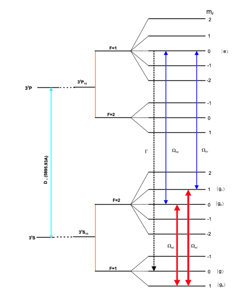
Figure 1: Linkages for quartuplet spectrum of four fields and four strongly-coupled levels of the Sodium atom. Spontaneous emission from state $\left|e\right\rangle,$ shown as a dashed linkage, is responsible for the spectrum

III The Autler-Townes quartuplet Spectroscopy

We propose a five-level atom with four as ground states hyperfine quadruplet and one excited state driven resonantly by two coherent and two microwave fields appropriately (see Fig. 1). Two pairs i.e., $\left|g_{1}\right\rangle$—$\left|g_{3}\right\rangle$ and $\left|g_{3}\right\rangle$—$\left|g_{2}\right\rangle$ of the four ground hyperfine energy states $\left|g_{1}\right\rangle$, $\left|g_{2}\right\rangle$, $\left|g\right\rangle$, $\left|g_{3}\right\rangle$ are driven by two microwave fields having Rabi frequencies $\Omega_{m_{1}}$ and $\Omega_{m_{2}}$ respectively. Similarly the excited state $\left|e\right\rangle$ is coupled with the ground states $\left|g_{1}\right\rangle$ and $\left|g_{2}\right\rangle$ by two coherent driving fields having Rabi frequencies $\Omega_{o_{1}}$ and $\Omega_{o_{2}}$. The system forms the shape of loop structured configuration under these steps. Furthermore the level $\left|e\right\rangle$ is also coupled with the level $\left|g\right\rangle$ via vacuum field modes. The coupling of the vacuum field modes only to this particular transition is reasonable, as in proposed configuration all transitions from the other states to $\left|g\right\rangle$ are dipole forbidden. The naturally existing one decay processes makes our system the simplest ones due to the simply probability loss. This will leads to some ideal behavior regarding the quartuplet spectroscopy which is necessary for defining the fundamental of this system. More later, at the end of this section we match this scheme with current experiments that may capable us to realize the results of this spectroscopy in a laboratory. We also consider the resonant atom-field interaction therefore, the interaction picture and the rotating wave picture coincide for the coherent couplings. The Hamiltonian under the interaction picture for the rotating wave and dipole approximation is now given by

$$\mathcal{H}(t)=\mathcal{H}_{A}+\mathcal{H}_{B}\left(t\right),$$ (1)

where

$$\mathcal{H}_{A} =\hbar(\Omega_{o_{1}}\left|e\right\rangle\left\langle g_{1}\right|+\Omega_{o_{2}}\left|e\right\rangle\left\langle g_{2}\right|+\Omega_{m_{1}}\left|g_{1}\right\rangle\left\langle g_{3}\right|+\Omega_{m_{2}}\left|g_{2}\right\rangle\left\langle g_{3}\right|)+H.C.,$$ (2)

$$\mathcal{H}_{B}\left(t\right) =\hbar\sum\limits_{k}g_{k}e^{i\Delta_{k}t}\left|e\right\rangle\left\langle g\right|a_{k}+H.C.$$ (3)

In Eq. (3), $g_{k}$ is the coupling constant between the $k$th mode and the atomic dipole moment between level $\left|e\right\rangle$ and level $\left|g\right\rangle$ while $\Delta_{k}=\omega_{eg}-\nu_{k}$ is the detuning of the $k$th mode with respect to the central frequency. Moreover, $a_{k}$ and $a_{k}^{\dagger}$ are the annihilation and creation operators, respectively. The statevector of the system at any time $t$ is given by

$$\left|\Psi(t)\right\rangle=[E(t)\left|e\right\rangle+G_{1}(t)\left|g_{1}\right\rangle+G_{2}(t)\left|g_{2}\right\rangle+G_{3}(t)\left|g_{3}\right\rangle]\left|\mathbf{0}\right\rangle+\sum\limits_{k}G_{k}(t)\left|g\right\rangle\left|1_{k}\right\rangle,$$ (4)

where $\left|\mathbf{0}\right\rangle$ denotes the absence of photons in all vacuum modes and $\left|1_{k}\right\rangle$ represents a single photon in the vacuum modes. In the infinite volume limits and apart from the proportionality factor the spontaneous emission spectrum can be obtained as (see Appendix-A),

$$S(\Delta)=\frac{\left|g\right|^{2}\Delta^{2}(\Delta^{2}-\left|\Omega_{m_{1}}\right|^{2}-\left|\Omega_{m_{2}}\right|^{2})^{2}}{(\Delta^{4}-\Delta^{2}\left|\Omega\right|^{2}+\left|\Omega_{o_{2}}\right|^{2}\left|\Omega_{m_{2}}\right|^{2}+\left|\Omega_{o_{1}}\right|\left|\Omega_{o_{2}}\right|\left|\Omega_{m_{1}}\right|\left|\Omega_{m_{2}}\right|\sin\varphi)^{2}+\frac{\Gamma^{2}}{4}(\Delta^{2}-\left|\Omega_{m_{1}}\right|^{2}-\left|\Omega_{m_{2}}\right|^{2})^{2}}.$$ (5)

Here we have replaced the set of discrete mode frequency $\nu_{k}$ by a continuum-field frequency $\omega,$ with that we have replaced the discrete set of detnings $\Delta_{k}$ by continuum variable $\Delta=\omega_{eg}-$ $\omega.$ We have also taken the continuum to have a uniform coupling to state $\left|d\right\rangle$ and have therefore replaced $g_{k}$ by a mode-dependent $g$ (not similar with the state $\left|g\right\rangle$). Also, in the Eq. (5), $\left|\Omega\right|=$ $\sqrt{\left|\Omega_{o_{2}}\right|^{2}+\left|\Omega_{m_{1}}\right|^{2}+\left|\Omega_{m_{2}}\right|^{2}}$ appears for the effective Rabi-frequency of the system. The spectrum vanishes when $\Delta=0,$ $\pm\sqrt{\left|\Omega_{m_{1}}\right|^{2}+\left|\Omega_{m_{2}}\right|^{2}}$, yielding three dark lines in the spectrum dividing it into four spectral components. The height of all the spectral components are the same and can be calculated from the expression $\frac{4\left|g_{k}\right|^{2}}{\Gamma^{2}}$. During the derivation of the spectrum relation we assumed that the atom is initially prepared in the excited state $\left|e\right\rangle$. This way of handling the problem is mathematically correct for the ideal behavior. However, physically it might be difficult to place an atom in its excited state as soon as the atom enters the cavity to interact with other driving fields. Thus from experimental point of view we ought to add the techniques or the mechanism of the process to prepare an atom in its excited state. This can be done very easily by coupling another field with the ground energy level and the level where the atom is required to prepare. This act will then bring the system into the context of resonance fluorescence where the results obtained under strong field limit will not match with the expected results of our system. However, the results obtained will match under weak field limit, in which the added field strength must be comparable with the decay rates, a well known phenomenon of resonance fluorescence in quantum optics. Hence the assumption of initial state preparation is reasonable and experimentally incorporable. In our system we selected a particular nature of the interaction of the driving fields with the atom to form a loop preserving the phase effect in the system. Each single phase, when treated separately, has a similar effect. However, if two or more of the phases are varied relatively, the result obtained may not match with the ones in which the phases vary separately. In our analysis we deal only with one phase for its effect on the system.

To support the physical aspect regarding the dressing of bare energy state into multiple components we define the state function of the system in terms of dressed state basis having eigen states $\left|\alpha\right\rangle,$ $\left|\beta\right\rangle,$ $\left|\gamma\right\rangle$ and $\left|\delta\right\rangle$ with their corresponding eigenvalues $\xi_{1}$, $\xi_{2}$, $\xi_{3}$ and $\xi_{4}$, as

$$\left|\Psi(t)\right\rangle = [\alpha_{k}\left(t\right)\left|\alpha\right\rangle+\beta_{k}\left(t\right)\left|\beta\right\rangle+\gamma_{k}\left(t\right)\left|\gamma\right\rangle+\delta_{k}\left(t\right)\left|\delta\right\rangle]\left|0\right\rangle$$ (6)

$$+\sum_{k}G_{k}(t)\left|g\right\rangle\left|1_{k}\right\rangle,$$

where

$$\mathcal{H}_{A}\left|\alpha\right\rangle =\hbar\xi_{1}\left|\alpha\right\rangle,$$ (7)

$$\mathcal{H}_{A}\left|\beta\right\rangle =\hbar\xi_{2}\left|\beta\right\rangle,$$ (8)

$$\mathcal{H}_{A}\left|\gamma\right\rangle =\hbar\xi_{3}\left|\gamma\right\rangle,$$ (9)

$$\mathcal{H}_{A}\left|\delta\right\rangle =\hbar\xi_{4}\left|\delta\right\rangle.$$ (10)

The eigenvalues appearing in the Eqs. (7-10) are the roots of characteristic equation of this system while the dressed states can be found by the usual way. These eigenvalues associated with the dressed states are also the roots of $D\left(\Delta_{k}\right)$ of the denominator of Eq. (A6) mentioned in the Appendix-A, using the bare energy state-vector approach. Thus the dressed statevector approach coincides with the bare statevector at least for the association of the number of bright spectral lines in the emission spectrum with the dressed states defined for this system (see Fig. 2). Satisfactorily, we will use the terminology of dressed states frequently for the explanation of our main results obtained by the bare statevector approach. The detailed analysis for the physical processes of the system in terms of dressed states basis is beyond the aim of this paper and will be discussed elsewhere. However, the analysis of our main results using bare statevector explains almost all the underlying physics of our system.

Next we continue with our bare statevector approach. To explore many facts about the mechanism involved in the phenomenon of quantum interference among the four decaying dressed states, we rewrite the above Eq. (5) in the following form

$$S(\Delta)\varpropto\sum_{i=1}^{4}\left|\frac{g^{\ast}}{\digamma}\frac{\xi_{i}(\xi_{i}^{2}-\left|\Omega_{m_{1}}\right|^{2}-\left|\Omega_{m_{2}}\right|^{2})\zeta_{i}}{\Delta-\xi_{i}}\right|^{2},$$ (11)

where the factor $\digamma$ and the factors $\zeta_{i}$ $\left(i=1-4\right)$ are given in the Appendix-A. $\xi_{i}$ $(i=1-4)$ as discussed earlier, are the roots of the following equation

$$\Delta^{4}-\Delta^{2}\left|\Omega\right|^{2}+\left|\Omega_{o_{2}}\right|^{2}\left|\Omega_{m_{2}}\right|^{2}+\left|\Omega_{o_{1}1}\right|\left|\Omega_{o_{2}}\right|\left|\Omega_{m_{1}}\right|\left|\Omega_{m_{2}}\right|\sin\varphi$$

$$+i\frac{\Gamma}{2}\Delta(\left|\Omega_{m_{1}}\right|^{2}+\left|\Omega_{m_{2}}\right|^{2}-\Delta^{2})=0.$$ (12)

The analysis of the Eqs. (11,12) leads us to interpret the phenomenon of quantum interference among the decaying dressed states in a more clear and transparent way. Since, the spontaneous emission intensity is proportional to the steady state of the absolute square of the probability amplitude $G_{k}(t\rightarrow\infty)$ (see Appendix A) in continuum limit. The continuum limit of the spectrum at detuning $\Delta,$ which is now proportional to $\left|G(\infty)\right|^{2}$ contains four absolute squared terms and twelve interference terms. The four absolute squared terms can be associated with four emission probabilities from the four dressed states of the bare energy state created by the atom-field interaction. The interference terms are contributed by the pathways among the upper excited four decaying dressed energy states. We note that the interference terms compensate the contribution from the absolute squared terms at the location $\Delta$ = $0,$ $\pm\sqrt{\left|\Omega_{m_{1}}\right|^{2}+\left|\Omega_{m_{2}}\right|^{2}}$. The spectrum becomes zero at these values leading to three dark lines in the total spectrum.

For appropriate choices of different spectroscopic parameters, the Eqs. (11)-(12) get the following shape

$$S(\Delta)=\Gamma\sum_{i=1}^{4}\left|\frac{\alpha_{i}+i\beta_{i}}{\Delta-(\alpha_{i}^{\prime}+i\beta_{i}^{\prime})}\right|^{2},$$ (13)

where in the Eq. (13), $\alpha_{i}$, $\beta_{i}$, $\alpha^{\prime}{}_{i}$, and $\beta^{\prime}{}_{i}$ $(i=1-4)$ are the appropriate integer values obtained due to specific choices of spectroscopic variables i.e., all the Rabi-frequencies and the decay rate in Eqs. (11,12). This equation is totally the numerical version of Eq. (10). Eq. (11) consists of four terms. Each term further consists of a numerator and a denominator. Each numerator and denominator if subjected to the selected variables of the system for the analysis of some behavior of the system then these terms appear as a complex numbers with the real and imaginary parts as real values. Thus as whole the spectrum appears as shown by Eq. (13). Here for each set of the system variables we estimates the FWHM of each spectral components. These estimation for various data are displayed in the form of numerical values in the discussion parts showing the validity of the Weisskopf-Wigner theory. These integer values appearing in the Eq. (13) are different for the different sets of these spectroscopic variables chosen for exploration of some behavior in the system. Now, we can readily estimate the peaks height, their locations and widths from the absolute squared terms. The spectrum therefore consists, in general, of four peaks locating at $\delta=\alpha_{i}^{\prime}$ with peak heights $(\alpha_{i}^{2}+\beta_{i}{}^{2})/\beta_{i}^{\prime 2}$ for $i=1-4$, respectively.

Figure 2: Schematic diagram of dressed-state energies and spontaneous emission transitions (dashed arrows) from these to the ground state. The dressed states are evenly spaced only when all the Rabi frequencies are equal. The dressed states of this figure are those associated with Fig. 3 frame (a). The corresponding dressed state diagram for the quintuplet spectrum Fig. 5 frames (a) and (b) has five equidistant dressed states and five spectral lines

Next we discuss the experimental feasibility of our loop structured five-level atomic scheme. We select the Sodium D1 line having two fine structured energy levels. Each state further splits into two hyperfine energy levels according to the usual coupling of the nuclear magnetic moment associated with the Sodium nuclear spin and the internal atomic magnetic field by the total electronics angular momentum of the orbital spinning electron. For each hyperfine level, the F quantum number further splits into $m_{F}=(2F+1)$ hyperfine sub-energy-level due to the Earth magnetic field of strength 1 Gauss. Therefore, the Sodium $D1$ line has a total of 16 sub-energy level lines with 12 allowed transitions due selection and polarization rules of Zeeman lines of a dipole transition. The hyperfine Zeeman splitting within each hyperfine state of the $D1$ line all lies in lower-frequency range of Radio frequency (RF) range i.e., $0.5$ $\sim$ $2.8$ MHz. However the typical value of Rabi frequency of a pulsed laser range from microwave ($\mathbf{\sim}$10 MHz) to Infrared range (1 THz). The values of the splitting of the hyperfine in the excited state is $189$ MHz while for the ground state it is of order of $1772$ MHz, a significantly large splitting. Both are in the range of lower frequency side of the microwave. Therefore, it is reasonable to couple the ground hyperfine energy levels with microwave fields. The excited allowed Zeeman energy levels of the $3P_{1/2}$ state can then be coupled with the grounded hyperfine Zeeman energy levels by optical frequency ranged laser fields. The simplification of the sixteen lines of the Sodium $D1$ into four hyperfine states have also been proposed in literature Fry ; Fry01 . The arguments employed are depended on linear polarization rules and the selection rules of the magnetic dipole allowed transitions. Extending to five-level atomic we select the four ground states of D1 lines i.e., $\left|3S_{1/2},F_{2}=2,m_{F}=1\right\rangle\Leftrightarrow\left|g_{1}\right\rangle,$ $\left|3S_{1/2},F_{2}=2,m_{F}=0\right\rangle\Leftrightarrow\left|g_{2}\right\rangle,$ $\left|3S_{1/2},F_{1}=1,m_{F}=1\right\rangle\Leftrightarrow\left|g_{3}\right\rangle$ and one excited state $\left|3P_{1/2},F_{1}=1,m_{F}=0\right\rangle\Leftrightarrow\left|e\right\rangle.$ The states $\left|3S_{1/2},F_{2}=2,m_{F}=1\right\rangle\Leftrightarrow\left|g_{1}\right\rangle$ and $\left|3S_{1/2},F_{2}=2,m_{F}=0\right\rangle\Leftrightarrow\left|g_{2}\right\rangle$ are coupled with the state $\left|3S_{1/2},F_{1}=1,m_{F}=1\right\rangle\Leftrightarrow\left|g_{3}\right\rangle$ by two microwave fields while they are coupled with the excited decaying state $\left|3P_{1/2},F_{1}=1,m_{F}=0\right\rangle\Leftrightarrow\left|e\right\rangle$ by two optical fields. The linkage of the excited state $\left|3P_{1/2},F_{1}=1,m_{F}=0\right\rangle\Leftrightarrow\left|e\right\rangle$ is considered with the ground state, $\left|3S_{1/2},F_{1}=1,m_{F}=0\right\rangle\Leftrightarrow\left|g\right\rangle$ via vacuum field modes. It is noteworthy to mention that in our scheme the order of energy levels does not matter as we considering resonant atom fields interaction. The linkages of the closely spaced hyperfine states by microwave fields are usual in literature. For example, the upper two closely spaced decaying levels of the model scheme of quantum beat laser are prepared in coherent superposition by a microwave field. In our system the one linkage of the optical linkages is dipole forbidden following the selection rules of the Zeeman splitting. However, there are experimental and theoretical methods where the linkages between the dipole forbidden transition may be made allowed by applying small statics magnetic of strength up to $1.2$ $mT$. For examples, the dipole forbidden transition in the Alkaline earth elements can be allowed by the linkage of this low statics electric field with appropriate levels, an experimental fact Barber . Moreover, in the model scheme of Correlated Spontaneous Emission (CEL) Laser the dipole forbidden states are coupled with a strong coherent field to prepare the system in coherent superposition of the upper and the ground states of the cascaded three-level atomic system. However, the involvement of one decay process in this quartuplet system makes it an ideal ones to have ideal behavior for defining the fundamentals of even this complicated spectroscopy. This simply loss system is very much important as there is no simple mechanism in literature (to the best of my knowledge) to control the spontaneous decay in a system. Moreover, the multiple ground states implementation for an atomic system are considered both theoretically copy and experimentally Xia . Next we discuss the experimental adjustability of our scheme with a very important experiment conducted recently for multi-wave mixing reported in Zanch . In the experiment they achieved eight-wave mixing in sodium atom having a folded five-level in the fine structure sodium atom. They suggested that their experiment is important for the future work and might be helpful for the coherent transient spectroscopy, Autler-Townes spectroscopy and EIT. Having the facilities of the linkages of multiple fields with the sodium atom it will be easy to go from fine to hyperfine Zeeman splitting in the Sodium D1 line due the technological facilities of the multiple-field couplings. We are required to link two microwave fields and two optical fields with the selected energy levels of the sodium D1 line for our system. The initially prepared excited state is then allowed to decay steadily to record the spectrum.

Having quantum interference as a basic processes in the Autler-Townes multiplet spectroscopy we make a distinction with the coherent population trapping (CPT), a phenomenon also arising of the same effect in the spontaneous emission studies Zhu-Scully ; Paspalakis ; Xia ; Mart . The area under the curve of spontaneous emission spectrum in the case of CPT is always less than the case when there is no quantum interference in the system. However, here in the Autler-Townes spectroscopy, there are dark lines in the spectrum arising because of quantum interferences among the decaying dressed states. The area under the curve in this case is almost the same as the one obtained from the Lorentzian line shaped spectrum associated with a decaying bare energy state without its dressing. This fact is also evident from our multiplet schemes where the sum of the full width at half maximum (FWHM) of all the spectral components are always almost equal to Einstein’s decay rate, $\Gamma$, a decay rate that is normally associated with a decaying bare energy state without its dressing. The area under the curves of the spontaneous emission spectrum which representing the energy given out by the atom to environment are same in the case of Autler-Townes spectrum but not in the CPT case. This means some population is always trapped in an upper excited dressed energy state in CPT while almost no population trapping is there in Autler-Townes multiplet spectroscopy. In both the CPT and Autler-Townes multiplet spectra there is quantum interference but their approaches are different regarding its effect. In the later case there are dark lines in the spectrum of Lorentzian line-shape while in the former there is complete elimination (and not control) of a spectral component.

IV The Autler-Townes Quintuplet Spectroscopy

Next, we modify our previous scheme for Autler-Townes quintuplet spectroscopy. These modifications can be carried in the previous system with a view to have a loop structured atom fields interaction. However, the needed single looped atom fields interaction is not unique and the problem can also be dealt for at least one loop in order to preserve the phase effect in the system. Therefore the higher odd-ordered multiplet schemes can be handled through branches and loops if and only if there is no parity violation. In the present scheme, we select one branch and one loop to preserve the phase effect. Therefore, we consider a six-level atom having five hyperfine ground energy states. The three pairs $\left|g_{1}\right\rangle$—$\left|g_{3}\right\rangle$, $\left|g_{3}\right\rangle$—$\left|g_{2}\right\rangle$ and $\left|g_{2}\right\rangle$—$\left|g_{4}\right\rangle$ of the four ground states are coupled resonantly with three microwave fields having the Rabi frequencies $\Omega_{m_{1}}$, $\Omega_{m_{2}}$ and $\Omega_{m_{3}}$ respectively. Similarly the ground states $\left|g_{1}\right\rangle$ and $\left|g_{2}\right\rangle$ are coupled resonantly with the excited state $\left|e\right\rangle$ by two optical driving fields having the Rabi frequencies$\ \Omega_{o_{1}}$and $\Omega_{o_{2}}$ respectively. The structure of this atom field interaction form a branch and a loop configurations (see Fig. 3). We expect same results if the structure of the atom-field interaction is kept in one loop shape. However, we are following the branch and the loop structure to have the different possibility of getting almost the same type results. Moreover, to include the unique allowed decay process in the system the level $\left|e\right\rangle$ is coupled with the level $\left|g\right\rangle$ via vacuum field modes. Later, at the end of this section we discuss the possibility of utilizing the experiment of Ref. Zanch for this quintuplet scheme and give a proposal of its adjustability for the realization using hyperfine D1 line of Sodium. The interaction picture Hamiltonian in the dipole and rotating wave approximation is then given by

$$\mathcal{H}(t)=\mathcal{H}_{A}+\mathcal{H}_{B}\left(t\right),$$ (14)

where

$$\mathcal{H}_{A} =\hbar(\Omega_{o_{1}}\left|e\right\rangle\left\langle g_{1}\right|+\Omega_{o_{2}}\left|e\right\rangle\left\langle g_{2}\right|+\Omega_{m_{1}}\left|g_{1}\right\rangle\left\langle g_{3}\right|+\Omega_{m_{2}}\left|g_{3}\right\rangle\left\langle g_{2}\right|$$

$$+\Omega_{m_{3}}\left|g_{2}\right\rangle\left\langle g_{4}\right|))+H.C.,$$ (15)

$$\mathcal{H}_{B}\left(t\right) =\hbar\sum\limits_{k}g_{k}e^{i\Delta_{k}t}\left|e\right\rangle\left\langle g\right|a_{k}+H.C.$$ (16)

The state-vector of the system at any time t is given by

$$\left|\Psi(t)\right\rangle =[E(t)\left|a\right\rangle+G_{1}(t)\left|g_{1}\right\rangle+G_{2}(t)\left|g_{2}\right\rangle+G_{3}(t)\left|g_{3}\right\rangle+$$

$$+G_{4}(t)\left|g_{4}\right\rangle]\left|\mathbf{0}\right\rangle+\sum\limits_{k}G_{k}(t)\left|g\right\rangle\left|1_{k}\right\rangle,$$ (17)

where $\left|\mathbf{0}\right\rangle$ denotes the absence of photons in all vacuum modes and $\left|1_{k}\right\rangle$ represents a single photon in the vacuum modes. In the infinite volume limit and apart from the proportionality factor the spontaneous emission intensity for this quintuplet atomic system is proportional to the steady state of the absolute square of the probability amplitude $G_{k}(t\rightarrow\infty)$ [see Eq. (B9) of the Appendix A] in continuum limit. The continuum limit of the spectrum $S(\Delta)$ at detuning $\Delta,$ which is now proportional to $\left|G(\infty)\right|^{2}$ is obtained as,

$$S(\Delta)=\frac{\left|g\right|^{2}\Delta^{4}\left[\Delta^{2}-\left|\Omega_{A}\right|^{2}+\left|\Omega_{B}\right|^{4}\right]^{2}}{(\Delta^{5}-\Delta^{3}\left|\Omega\right|^{2}+\Delta\left|\Omega_{C}\right|^{4}+2\left|\Omega_{D}\right|^{5}\cos\varphi)^{2}+\frac{\Gamma^{2}}{4}\Delta^{4}\left[\Delta^{2}-\left|\Omega_{A}\right|^{2}+\left|\Omega_{B}\right|^{4}\right]^{2}},$$ (18)

where

$$\left|\Omega_{A}\right|^{2} =\left|\Omega_{m_{1}}\right|^{2}+\left|\Omega_{m_{2}}\right|^{2}+\left|\Omega_{m_{3}}\right|^{2},$$ (19)

$$\left|\Omega_{B}\right|^{4} =\left|\Omega_{m_{2}}\right|^{2}\left|\Omega_{m_{3}}\right|^{2},$$ (20)

$$\left|\Omega_{C}\right|^{4} =\left|\Omega_{o_{1}}\right|^{2}\left|\Omega_{m_{2}}\right|^{2}+\left|\Omega_{m_{1}}\right|^{2}\left|\Omega_{o_{2}}\right|^{2}+\left|\Omega_{m_{2}}\right|^{2}\left|\Omega_{m_{3}}\right|^{2}+\left|\Omega_{m_{3}}\right|^{2}\left|\Omega_{o_{2}}\right|^{2},$$ (21)

$$\left|\Omega_{D}\right|^{5} =\left|\Omega_{o_{1}1}\right|\left|\Omega_{m_{1}}\right|\left|\Omega_{m_{2}}\right|\left|\Omega_{m_{3}}\right|\left|\Omega_{o_{2}}\right|,$$ (22)

$$\left|\Omega\right| =\sqrt{\left|\Omega_{o_{1}}\right|^{2}+\left|\Omega_{m_{1}}\right|^{2}+\left|\Omega_{m_{2}}\right|^{2}+\left|\Omega_{m_{3}}\right|^{2}+\left|\Omega_{o_{2}}\right|^{2}},$$ (23)

Again, we have replaced the set of discrete mode frequency $\nu_{k}$ by a continuum-field frequency $\omega,$ for this system. Consequently we have replaced the discret set of detnings $\Delta_{k}$ by continuum variable $\Delta=\omega_{eg}-$ $\omega.$ We have also taken the continuum to have a uniform coupling to state $\left|g\right\rangle$ and have therefore replaced $g_{k}$ by a mode-dependent $g.$ Further, by inspection we note that the spectrum is vanished at the locations:

$$\Delta=\pm\frac{1}{\sqrt{2}}\sqrt{\left|\Omega_{A}\right|^{2}-\sqrt{\left|\Omega_{A}\right|^{4}-4\left|\Omega_{B}\right|^{4}},}$$ (24)

and

$$\Delta=\pm\frac{1}{\sqrt{2}}\sqrt{\left|\Omega_{A}\right|^{2}+\sqrt{\left|\Omega_{A}\right|^{4}-4\left|\Omega_{B}\right|^{4}}}.$$ (25)

Thus, yielding four dark lines in the spectrum dividing it into five spectral components. The height of all the spectral components are same and can be calculated from $\frac{4\left|g_{k}\right|^{2}}{\Gamma^{2}}.$

Again to explain the physical aspects regarding the dressing of bare energy state into multiple components we define the state function of the system in terms of five dressed-states basis having eigenstates $\left|\alpha\right\rangle$, $\left|\beta\right\rangle$, $\left|\gamma\right\rangle$, $\left|\delta\right\rangle$ and $\left|\epsilon\right\rangle$ with their corresponding eigenvalues $\xi_{1}$, $\xi_{2}$, $\xi_{3}$, $\xi_{4}$ and $\xi_{5}$, respectively

$$\left|\Psi(t)\right\rangle =[\alpha_{k}\left(t\right)\left|\alpha\right\rangle+\beta_{k}\left(t\right)\left|\beta\right\rangle+\gamma_{k}\left(t\right)\left|\gamma\right\rangle$$

$$+\delta_{k}\left(t\right)\left|\delta\right\rangle+\epsilon_{k}\left(t\right)\left|\epsilon\right\rangle]\left|0\right\rangle+\sum_{k}G_{k}(t)\left|g\right\rangle\left|1_{k}\right\rangle,$$ (26)

where

$$\mathcal{H}_{A}\left|\alpha\right\rangle =\hbar\xi_{1}\left|\alpha\right\rangle,$$ (27)

$$\mathcal{H}_{A}\left|\beta\right\rangle =\hbar\xi_{2}\left|\beta\right\rangle,$$ (28)

$$\mathcal{H}_{A}\left|\gamma\right\rangle =\hbar\xi_{3}\left|\gamma\right\rangle,$$ (29)

$$\mathcal{H}_{A}\left|\delta\right\rangle =\hbar\xi_{4}\left|\delta\right\rangle,$$ (30)

$$\mathcal{H}_{A}\left|\epsilon\right\rangle =\hbar\xi_{5}\left|\epsilon\right\rangle.$$ (31)

The eigenvalues appearing in the Eqs. (27-31) are the roots of the characteristics equation of this system and are also the roots of $D\left(\Delta_{k}\right)$ appeared in the Eq. (B9) of the Appendix-B while these dressed states can be calculated by the usual way. For this system the dressed statevector approach also coincides with the bare statevector at least for the association of the five bright spectral lines in the emission spectrum with the five dressed states defined for this system. Again, we are safe to use the terminology of the dressed states for the explanation of the results obtained under the bare statevector approach.

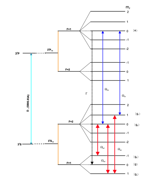
Figure 3: Linkages for quintuplet spectrum of five fields and five strongly-coupled levels of the Sodium atom. The spontaneous emission from state $\left|e\right\rangle$ of the quintuplet, shown as a dashed linkage, is responsible for the spectrum

To continue the discussion, we proceed with bare energy statevector approach. Further, to understand and explain the physical processes of the quantum interference with a view of the dressing of the bare energy, the Eq. (18) is rewritten as

$$S(\Delta)\varpropto\sum_{i=1}^{5}\left|\frac{g^{\ast}}{\Lambda}\frac{[\left|\Omega_{B}\right|^{2}-\left|\Omega_{A}\right|^{2}\xi_{i}^{2}+\xi_{i}^{4}]\kappa_{i}}{\Delta-\xi_{i}}\right|^{2},$$ (32)

where $\xi_{i}$ $\left(i=1-5\right)$ are the roots of the equation

$$(\Delta^{5}-\Delta^{3}\left|\Omega\right|^{2}+\Delta\left|\Omega_{C}\right|^{4}+2\left|\Omega_{D}\right|^{5}\cos\varphi)^{2}+\frac{\Gamma^{2}}{4}(\Delta^{4}-\Delta^{2}\left|\Omega_{A}\right|^{2}+\left|\Omega_{B}\right|^{4})^{2}=0,$$ (33)

and the factor $\Lambda$ and the factors $\kappa_{i}$ $\left(i=1-5\right)$ are given in the Appendix-B. Further, Eqs. (32,33) are now again simply to read. The spectrum relation contains five absolute squared terms and twenty interference terms. The five absolute squared terms are associated with five emission probabilities from the set of five dressed state of the bare energy state having no dark lines in the spectrum. The twenty interference terms are contributed by the five pathways among the upper excited decaying dressed states responsible for generating the four dark lines in the total spectrum of the system. We note that the interference terms compensate the contribution from the absolute squared terms at the locations given by the Eqs. (24,25).

For appropriate choices of different spectroscopic variables Eqs. (34,35) get the following shape

$$S(\Delta)=\Gamma\sum_{i=1}^{5}\left|\frac{\alpha_{i}+i\beta_{i}}{\Delta-(\alpha_{i}^{\prime}+i\beta_{i}^{\prime})}\right|^{2},$$ (34)

where in the above equation $\alpha_{i}$, $\beta_{i}$, $\alpha_{i}^{\prime}$, and $\beta_{i}^{\prime}$ $(i=1-5)$ are the appropriate integer values obtained due to specific choices of spectroscopic variables of this system. Therefore, we can again readily estimate the peaks height, their locations and their widths from the absolute squared terms. The spectrum therefore consists of in general, five peaks located at $\Delta=\alpha_{i}^{\prime}$ $(i=1-5)$ while the heights of the peaks locating at $\alpha_{i}^{\prime}$ are given by $(\alpha_{i}^{2}+\beta_{i}{}^{2})/\beta_{i}^{\prime 2}$ for $i=1-5$.

We again utilize the Sodium atom in its hyperfine Zeeman states of the D1 lines. Extending to six-level atomic system we select the five ground states of D1 lines i.e., $\left|3S_{1/2},F_{2}=2,m_{F}=1\right\rangle\Leftrightarrow\left|g_{1}\right\rangle,$ $\left|3S_{1/2},F_{2}=2,m_{F}=0\right\rangle\Leftrightarrow\left|g_{2}\right\rangle,$ $\left|3S_{1/2},F_{1}=1,m_{F}=1\right\rangle\Leftrightarrow\left|g_{3}\right\rangle,$ $\left|3S_{1/2},F_{1}=2,m_{F}=-1\right\rangle\Leftrightarrow\left|g_{4}\right\rangle$ and one excited state $\left|3P_{1/2},F_{1}=1,m_{F}=0\right\rangle\Leftrightarrow\left|e\right\rangle.$ The states $\left|3S_{1/2},F_{2}=2,m_{F}=1\right\rangle\Leftrightarrow\left|g_{1}\right\rangle$ and $\left|3S_{1/2},F_{2}=2,m_{F}=0\right\rangle\Leftrightarrow\left|g_{2}\right\rangle$ are coupled with the state $\left|3S_{1/2},F_{1}=1,m_{F}=1\right\rangle\Leftrightarrow\left|g_{3}\right\rangle$ by two microwave fields while they are coupled with the excited decaying state $\left|3P_{1/2},F_{1}=1,m_{F}=0\right\rangle\Leftrightarrow\left|e\right\rangle$ by two optical fields. In addition to this we couple another microwave field with the transition $\left|3S_{1/2},F_{2}=2,m_{F}=0\right\rangle\Leftrightarrow\left|g_{2}\right\rangle\Leftrightarrow\left|3S_{1/2},F_{1}=1,m_{F}=-1\right\rangle\Leftrightarrow\left|g_{4}\right\rangle$. Like the previous scheme here the linkage of the excited state $\left|3P_{1/2},F_{1}=2,m_{F}=0\right\rangle\Leftrightarrow\left|e\right\rangle$ is also considered with the ground state, $\left|3S_{1/2},F_{1}=1,m_{F}=0\right\rangle\Leftrightarrow\left|g\right\rangle$ via vacuum field modes. It is again noteworthy to mention that in our scheme the order of energy levels does not matter as we considering resonant atom fields interaction.The nomenclature of this form the shape of a loop and a branch, another possibility of the atom-field interaction. The same experiment of Ref. Zanch is equally useful for demonstration of the results of quintuplet spectroscopy. Here we are need to couple another microwave field with the additional ground energy level to have five ground states. Although, the atom-field interaction forming the configuration of a branch and a loop however, the order of energy levels does not affect the end results for resonant atom-field interaction of this system. Now, we need to record the spectrum when the atom decay from the excited state to the ground.

V Autler-Townes Sextuplet and Higher-Ordered Multiplet Spectroscopy

In this section we suggest the general nomenclatures for the sextuplet and consequently for the higher-ordered multiplet Autler-Townes atomic schemes. From the successive study of Autler-Townes spectra from the doublet to the quintuplet we come to know that going from a lower to a next higher-ordered spectrum we need to increase the number of atomic states by one interacting with the required number of fields to have the required coupling states. If there are N coupled states then there is the generation of N dressed states associated with the decaying bare state of the scheme under investigation regardless of the number of fields. Generally this procedure is necessary to increase the number of dressed states by one. In this way we may be able to split the decaying bare energy state to any number of dressed energy state depending on the number of energy levels of the atomic system, the nature of the required fields and the nature of their interaction. Earlier, in our previously proposed schemes for the quartuplet and quintuplet spectroscopy we based our schemes on D1 line of the hyperfine-structured Sodium atom to have simple probability loss. Due to this plausible simplification, the atomic systems are the ideal one having one decaying levels and are handled analytically by a statevector method even for these complicated systems. It worthy to mention that these simplified systems are necessary for displaying the ideal behavior. The potentiality of these systems is unquestionable because the multiple uncontrollable decaying processes may lead to complications to disturb the ideal behavior of the involved dynamics in the systems under investigation. The states of these simple schemes correspond to pure states and the obtained results are mathematically very easy to explain various aspects of the phenomenon of spontaneous emission processes in the higher-ordered multiplet spectroscopy.

To go beyond and to suggest schemes of higher-ordered multiplet spectrum, for example the sextuplet atomic scheme, we need six ground hyperfine energy states and an excited energy state of the sodium atom. Luckily this type of nomenclature can also be found in the sodium D1 lines in hyperfine Zeeman splitting. Six ground states can be selected from the eight closely spaced Zeeman levels associated with the lower level of the fine energy level of the sodium D1 line and one from the allowed ones of the excited states. This seven energy states scheme can be driven by two optical and five microwave fields either in a loop or a loop plus a branch structured configuration using the real sodium atom. This then forms a scheme of having simple probability loss and can be handled by the previously presented approach to have ideal behavior. Due to this atom-field interaction, the only one decaying bare energy states will split into six dressed energy states which will then interfere destructively among themselves to create five dark lines in the spectrum. These dark lines will then divide the spectrum into six components.

Furthermore, if the fine structured sodium atom is considered, for example the ones of Zuo et al. which requires a loop plus a branch structured involving three decay rates such that the system is strictly subjected to the resonant atom-field interaction with no requirement of microwave fields. The configuration then forms the shape of folded NV shaped atomic system. This scheme involves three decay processes and corresponds to a mix state and may not be handled by the previously presented statevector approach.

The system becomes more complicated due to the next increase in the number of coupled atomic energy levels and the increase in the number of the driven laser fields for higher ordered multiplet spectroscopy. In this situation it will not be very easy to avoid decaying processes and the other processes of decoherence during an experiment and may affect the ideal behavior Zhu-Narducci ; Fazal . However, if these complications are very large in its rates then the decoherence processes may completely eliminate the dark lines feature from the spectra. The process of quantum destructive interference among the dressed energy states will then be completely washed out from the system. It will also become very hard to handle the problems with the statevector methods and may be dealt with the density matrix formalism or using generalized Bloch equations of motion for the system under investigation using numerical simulation. This idea is extendable into any higher-ordered multiplet spectrum. Proposing such a multiplet scheme requires careful selection of the laser fields, number of atomic energy levels of the atom or molecule and their appropriate interaction such that there is no violation of parity except the ones that nature permit.

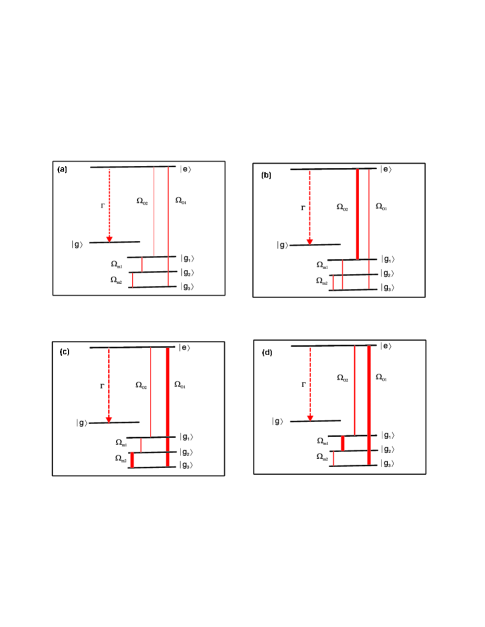
Figure 4: Linkage patterns and relative strengths of four driving fields for quartet spectra of Fig. 4. (a) all Rabi frequencies are equal to $0.5\Gamma$. (b) The single Rabi frequency $\left|\Omega_{o_{2}}\right|$ is $4\times$ the others. (c) Rabi frequencies $\left|\Omega_{o_{1}}\right|$ and $\left|\Omega_{m_{1}}\right|$ are $4\times$ the others. (d) Rabi frequencies $\left|\Omega_{o_{1}}\right|$ andr $\left|\Omega_{m_{2}}\right|$ are $4\times$ the others. In these linkage plots the vertical positions of the lines associated with energy states is irrelevant, unlike Fig. 1 where vertical position is associated with energy.

VI Discussion

In this section we discuss our main results presented in the text. In presenting these results we take support of the analytical results and the numerical estimations regarding various facts of Autler-Townes multiplets spectra. We specially underlined the techniques in the text that how the widths of all the spectral components (bright lines) in all the schemes can be estimated from the numerical analysis. We preferred this way of analysis as due to complex nature of atom-field interaction, the analytical forms of the widths of all spectral components in their corresponding schemes are very hard to calculate and are not presentable.

VI.1 The Quartuplet Spectrum

First of all we inspect the generality of quartuplet atomic system. The analytical result obtained for this system is given by Eq. (5). The atomic system reduces to a two-level atom interacting with the vacuum field modes when all the four laser fields are vanished. This results in a Lorentzian line-shape spectrum whose height is $4\left|g_{\mathbf{k}}\right|^{2}/\Gamma^{2}$ and the FWHM is $\Gamma$ Book1 . Furthermore, the result reduces to the form

$$S\left(\Delta\right)=\frac{\left|g\right|^{2}\Delta^{2}}{\left(\Delta^{2}-\left|\Omega_{o_{1}}\right|^{2}\right)^{2}+\frac{\Gamma^{2}}{4}\Delta^{2}}.$$ (35)

when only $\left|\Omega_{o_{2}}\right|$, $\left|\Omega_{m_{1}}\right|$ and $\left|\Omega_{m_{2}}\right|$ are set to zero. In this case the atomic system reduces to a three-level atom interacting with a laser field and results in the well known Autler-Townes doublet spectrum Zhu-Narducci showing its generality. Furthermore, this scheme cannot be reduced to the results of Autler-Townes triplet spectrum as all the atomic systems are subjected to no parity violation condition except the ones that nature permit. Therefore, there is symmetry among the even numbered Autler-Townes multiplet schemes when and only when the schemes are based on fine structured atomic system while avoiding the parity violations. The higher even numbered multiplet schemes then reduce to the analytical results of the preceding even numbered multiplet schemes. For example in the present case the results of the quartuplet spectrum is reduced to the results of doublet scheme as shown above. However, this symmetry is valid only for spectrum beyond Autler-Townes triplet in the present case.

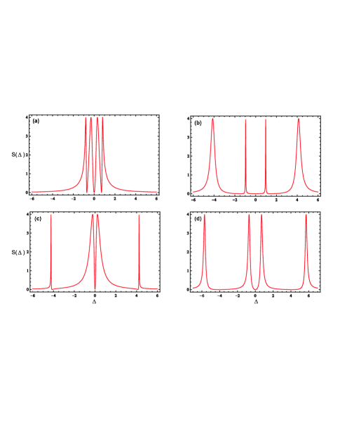
Figure 5: Quartuplet spectrum for four fields and five states for the linkages of Fig. 3 with phase $\varphi=2\pi$ and (a) $\left|\Omega_{o_{1}}\right|=\left|\Omega_{o_{2}}\right|=\left|\Omega_{m_{1}}\right|=\left|\Omega_{m_{2}}\right|=0.5\Gamma$. (b) $\left|\Omega_{o_{1}}\right|=\left|\Omega_{m_{1}}\right|=\left|\Omega_{m_{2}}\right|=1\Gamma$ and $\left|\Omega_{o_{2}}\right|=4\Gamma$. (c) $\left|\Omega_{o_{1}}\right|=\left|\Omega_{m_{1}}\right|=4\Gamma$ and $\left|\Omega_{o_{2}}\right|=\left|\Omega_{m_{2}}\right|=1\Gamma$. (d) $\left|\Omega_{o_{1}}\right|=\left|\Omega_{m_{2}}\right|=1\Gamma$ and $\left|\Omega_{o_{2}}\right|=\left|\Omega_{m_{1}}\right|=4\Gamma$.

Now we proceed with the discussion of the results for the quartuplet spectrum. In Fig. (4), we present the linkages of the driving fields with the atomic system according to our proposal presented in section 3. However, in these linkages plots the vertical positions of the lines associated with actual position in the sodium hyperfine structured atomic system is irrelevant. Also, in this quartuplet scheme, the linkages of the coherently strong driving fields associated with their respective Rabi frequencies are shown by the thick lines while the thin are shown for the weak fields under consideration. These are displayed for the better understanding of the physics of the spectrum for this quartuplet as the order of energy levels in the resonant atom-field interactions does not matter. We note that the three dark lines are always there regardless of the strengths of the four driving fields. The four spectral components can obviously be seen separated by the three dark lines at the locations $\Delta$ = $0,$ $\pm\sqrt{\left|\Omega_{m_{1}}\right|^{2}+\left|\Omega_{m_{2}}\right|^{2}}$ for the small values of the Rabi frequencies as shown in Fig. (5a). In Fig. (4a) the four equally linked weak fields with the atomic transition frequencies are shown by the thin lines. The spectral components are equally spaced on the frequency axis having small separation. These three dark lines appear due to the interference effect among the four decaying dressed states created by the atom-field interaction. One dark line is always located at the central line. However, the other two which lying symmetrically on the positive and negative frequency axes of the spectrum are effectively controlled by the variation of $\left|\Omega_{m_{1}}\right|$ and $\left|\Omega_{m_{2}}\right|$. This symmetry arises due to the resonance coupling of the driving fields with their respective atomic transitions frequencies. However, if the fields are detuned from these transitions then the spectrum will become asymmetric. Here, we limit our discussion only to the resonance cases due their various advantages. Further, both the dark lines and the effective Rabi frequency for this system are independent of the Rabi-frequency $\left|\Omega_{o_{1}}\right|$ which means that the quartuplet nature of the spectrum is not altering if $\left|\Omega_{o_{1}}\right|=0$. However, the phase dependent term, $\left|\Omega_{o_{1}}\right|\left|\Omega_{o_{2}}\right|\left|\Omega_{m_{1}}\right|\left|\Omega_{m_{2}}\right|\sin\varphi$ appearing at the denominator of the spectrum Eq. (5) is vanished eliminating the phase effect from the system. Therefore the loop structure of the atom-field interaction is important for the preserving the phase effect in the system, a parameter which may have numerous advantages for future studies related to this work Fazal111 . Furthermore, using Eq. (5) we note that the FWHM of these spectral components for the same strength of the driving laser fields are always the same and are equal to one-fourth of the Einstein’s decay rate $\Gamma.$ The sum of these widths is equal to $\Gamma$ which is the standard value as obtained by Weisskopf-Wigner theory for the spontaneous emission of two-level decaying atom due to vacuum. However, for stronger but same driving fields, the dark lines feature of the spectrum equally widens, with the expected behavior of the upper excited four dressed states, whose spacing are controlled by the Rabi frequencies of all the four driving fields. Moreover, the FWHM of each of the four spectral components in this case is also $\frac{\Gamma}{4}$ and obeying the Weisskopf-Wigner theory for its total width. Obviously, the shapes of the individual spectral component in these cases and in the coming up are not Lorentzian. They are the examples of Breit-Wigner or Fano profiles. It is now obvious to describe that when all the Rabi frequencies are equal then the widths of all the peaks are then all equal and they are separated equally by greater amounts. Consequently the peaks are more widely spaced while their widths are unaffected. Generally, in the quartuplet atomic scheme there are always four spectral lines separated by the dark lines and associated with the four dressed states created by the interaction of four fields with the atom. However, it is worthwhile to mention that the number of the dressed states and the number of the fields which are equal in this system, is accidental. In principle, one dressed state can be associated with one strongly linked state by the fields regardless of its numbers. If there are N linked atomic states with the driving fields then there must be N dressed states. For example, the very famous scheme for spontaneous emission cancellation Zhu-Scully ; Xia ; Mart involves only one field in a four level atomic system. However, the strong linkage of this single field with three atomic states creates three dressed states while there is only one driving field in the system. Another very famous scheme is the Autler-Townes doublet where single strong coherent driving field linked with the two bare states and thus generates two dressed states for the one decaying bare state.

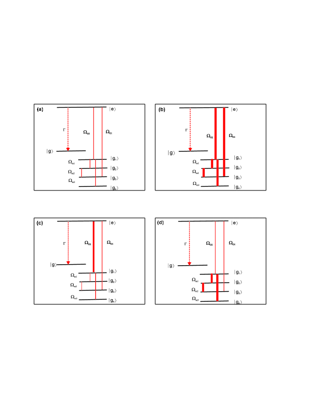
Figure 6: Linkage patterns and relative strengths of five driving fields for quintuplet spectra of Fig. 6. (a) all Rabi frequencies are equal to $0.5\Gamma$. (b) Rabi frequencies are strong, equal to $3\Gamma.$ (c) Rabi frequencies $\left|\Omega_{o_{2}}\right|$ is $4\times$ all the others. (d) Rabi frequencies $\left|\Omega_{m_{3}}\right|$, $\left|\Omega_{m_{2}}\right|$ and $\left|\Omega_{m_{1}}\right|$ are $4\times$ the others. In these linkage plots the vertical positions of the lines associated with energy states is irrelevant, unlike Fig. 2 where vertical position is associated with energy

Next, we explore the nature of the line-width narrowing and broadening in different spectral components of the emission spectra of the quartuplet scheme. We explain clearly the coherence effect of the driving fields and its distinction regarding the opposite effects of the line-width narrowing and broadening associated with their appropriate driven fields respectively. We note the extreme line width narrowing in all the four peaks of the spectrum with the change in relative strengths of the coherently driving fields. The detailed numerical analysis of the spectrum Eq. (11) for the different sets of parameters of the system variable leads us to a similar response as compared with the analytical results. The FWHM of the central two peaks associated with the two central dressed states of the set of four dressed states for the decaying bare energy state start to decrease with the increase of either $\left|\Omega_{o_{1}}\right|$ or $\left|\Omega_{0_{2}}\right|$. They become lesser and lesser with the more increase of the corresponding Rabi frequency as shown by the Fig. 5(b). The linkages of one strong field and three weak fields with atomic system are displayed in Fig. 4(b) by a thick line and three thin lines, respectively. This effect of spectral narrowing becomes double for both the central peaks when there is simultaneous increase in both the Rabi frequencies. However, the widths of the side peaks of the set of four dressed states become larger and larger accordingly. Furthermore, we also noticed that the decrease in widths of the two central peaks always compensates the increase in the widths of the side two peaks of the spectrum for both the individual or simultaneous increase of the Rabi frequencies. This is in accord with the theory of Weisskopf-Wigner and the sum of these widths is always equal to Einstein’s decay rate. The plot of the Eq. (5) manifests the behavior what we predicted from the numerical analysis of the widths of the four spectral components. The four linkages for the two weak fields and the two strong fields are also shown by the Fig. 4(c). Further, the widths of the two central peaks are always the same and these decreases to the same value of $0.05\Gamma$ for an optimum value of the Rabi frequency $\left|\Omega_{o_{1}}\right|$, while the widths of the side two peaks increase in the same proportion and is equal to $0.45\Gamma$ for each one respectively. The same effects are seen when $\left|\Omega_{o_{2}}\right|$ is increased instead of $\left|\Omega_{o_{1}}\right|.$ Moreover by increasing both the Rabi frequencies, the narrowing effect is doubled with the side peaks displaced more from the central one [see Fig. 5(c)]. While increasing the Rabi frequencies $\left|\Omega_{m_{1}}\right|$, $(\left|\Omega_{m_{2}}\right|)$ or both, the FWHM of the two central peaks of the set of four peaks of the spectrum starts to increase drastically with a double effect in the simultaneous case. However, it reduces the widths of the two side peaks correspondingly. As a result we obtain extreme line-width narrowing in the side two peaks and extreme line-width broadening in the two central peaks for optimum value of these Rabi frequencies. This increase and decrease in the two central and the two sides peaks are again always in the same proportion and obey Weisskopf-Wigner theory. The maximum possible increase in the widths of the two central peaks in this case is $0.45\Gamma$ for each one of the two, whereas for the sides peaks it decreases to $0.05\Gamma$ for each one of the two. However, when the linkages pattern of the driving fields like the one shown in the atomic scheme of Fig. 3(d), the spectrum displays irregular behavior regarding the widths of the four components of the spectrum and the position of the dark lines. The reason is obvious. The one stronger field having narrowing effect in one component compensate the broadening effect of the other equally stronger field on the same component see Fig. 5(d). However, the peaks take the position according to the strengths of the fields. The fields which are directly linked with the decaying level play the role of displacing away (closing together) the two central peaks while the fields which are not directly linked with the decaying level play the role in displacing away (closing together) the sides peaks of the spectrum when fields strength are increasing (decreasing). Physically, this is reasonable as the splitting of the dressed states are directly controlled by the strengths of the driving fields but in a symmetrical way. In fact, this is a relative phenomenon for this system regarding the effect of relative strengths on the spacing of the dressed states for this system. However, the combinational effect can then be dealt accordingly. This makes sense to having unequal spacing with the irregular strength of the driving fields avoiding the principle stated above. Further, it is also worthwhile to note that the numerical analysis of the widths of different spectral components is sufficient to explore the physics of spectral narrowing and broadening arises due to the quantum interference mechanism in the atomic system. However, it is not difficult to plot the response of widths with the different Rabi frequencies of the system by following the method discussed in Ref. Fazal00 .

VI.2 The Quintuplet Spectrum

The analytical results obtained for the quintuplet atomic system are given by the Eq. (18). This atomic system also reduces to a two level atom interacting with the vacuum fields when all the five laser fields are vanished. This results in a Lorentzian line-shape spectrum whose height is $4\left|g_{\mathbf{k}}\right|^{2}/\Gamma^{2}$ and the FWHM is $\Gamma$ Book1 . In this case too, the result reduces to the form of Autler-Townes doublet when the Rabi frequencies $\left|\Omega_{m_{1}}\right|$, $\left|\Omega_{m_{2}}\right|$, $\left|\Omega_{m_{3}}\right|$ and $\left|\Omega_{o_{2}}\right|$ in Eq. (18) become zero. Further when the Rabi frequencies $\left|\Omega_{o_{2}}\right|$ and $\left|\Omega_{m_{3}}\right|$ in the analytical expression of this system are set to zero then the spontaneous emission spectrum reduces to the expression of Autler-Townes triplet spectrum Fazal ; Fazal00 given by

$$S\left(\Delta\right)\varpropto\frac{\left|g\right|^{2}\left(\left|\Omega_{m_{1}}\right|^{2}-\Delta^{2}\right)^{2}}{\left(\Delta^{3}-\left(\left|\Omega_{o_{1}}\right|^{2}+\left|\Omega_{m_{1}}\right|^{2}+\left|\Omega_{m_{1}}\right|^{2}\left|\Omega_{m_{2}}\right|^{2}\right)\Delta\right)^{2}+\frac{\Gamma^{2}}{4}\left(\left|\Omega_{m_{1}}\right|^{2}-\Delta^{2}\right)^{2}}.$$ (36)

Furthermore, the quintuplet scheme cannot be reduced to the results of Autler-Townes quartuplet spectrum as all the systems are independent of parity violation. Therefore, there is symmetry among the odd numbered Autler-Townes multiplet schemes when and only when the schemes are based on the hyperfine structured atomic system having no parity violations. The analytical results for higher odd numbered schemes will reduce to the analytical results of the preceding odd numbered Autler-Townes multiplet schemes. For example in the present case the result of the quintuplet spectrum is reduced to the result of triplet scheme as shown above. However, this symmetry is valid only for spectrum beyond Autler-Townes quartuplet spectrum in the case of odd numbered Autler-Townes multiplet schemes.

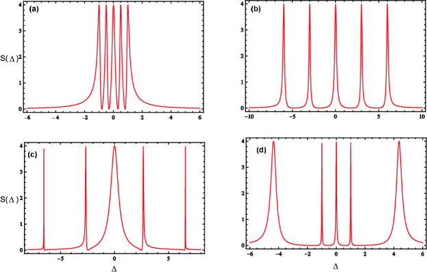
Figure 7: LQuaintuplet spectrum for four fields and five states for the linkages of Fig. 5 with phase $\varphi=2\pi$ and (a) $\left|\Omega_{o_{1}}\right|=\left|\Omega_{o_{2}}\right|=\left|\Omega_{m_{1}}\right|=\left|\Omega_{m_{2}}\right|=\left|\Omega_{m_{3}}\right|=0.5\Gamma$. (b) $\left|\Omega_{o_{1}}\right|=\left|\Omega_{o_{2}}\right|=\left|\Omega_{m_{1}}\right|=\left|\Omega_{m_{2}}\right|=\left|\Omega_{m_{3}}\right|=3\Gamma$. (c) $\left|\Omega_{o_{1}}\right|=4\Gamma$ and $\left|\Omega_{o_{2}}\right|=\left|\Omega_{m_{1}}\right|=\left|\Omega_{m_{2}}\right|=\left|\Omega_{m_{3}}\right|=1\Gamma$. (d) $\left|\Omega_{o_{1}}\right|=\left|\Omega_{o_{3}}\right|=1\Gamma$ and $\left|\Omega_{m_{3}}\right|=\left|\Omega_{m_{2}}\right|=\left|\Omega_{m_{3}}\right|=4\Gamma$.

In Fig. (5), we present the linkages of the driving fields with the atomic system proposed for this system. In these Linkages plots the vertical positions of the six lines associated with actual positions in the sodium hyperfine structured atom (see Fig. (3)) are irrelevant. In this quintuplet scheme, the linkages of the coherently strong driving fields associated with their respective Rabi frequencies are shown by the thick lines while they are thin for the weak fields. Here, we observed four dark lines in the spectrum irrespective of the strength of the five driving fields. The locations of these four dark lines can be inspected very easily from Eqs. (24,25) which split the spectrum into five spectral components as shown by the Fig. 7 (a). Their relevant linkages pattern for all the weak fields is shown in Fig. 7(a). The source of these dark lines is the interference mechanism among the five paths from the five dressed decaying states created by the atom-field interaction. Again, all the dark lines as well as the effective Rabi frequency are independent of Rabi-frequency $\left|\Omega_{o_{2}}\right|$ and means that the quintuplet nature of the spectrum is not altering if $\left|\Omega_{o_{2}}\right|=0$. However, the phase dependent term, $\left|\Omega_{o_{1}}\right|\left|\Omega_{m_{1}}\right|\left|\Omega_{m_{2}}\right|\left|\Omega_{m_{3}}\right|\left|\Omega_{o_{2}}\right|\cos\varphi$ appearing at the denominator of the spectrum Eq. (20) is vanished, washing out the phase effect from the system. Further, the naturally conversion of $\sin\varphi$ to $\cos\varphi$ in this system is satisfactory as the increase in the energy level of the system changes the origin of the phase by $\frac{\pi}{2}.$ This change in the phase arises due to the term in the calculations of the spectrum for the quintuplet scheme appearing as a complex conjugate when compared with its related term in the quartuplet scheme. The FWHM of each of the five spectral components for the same strength of the driving laser field is always the same and is equal to $\frac{\Gamma}{5}.$ The sum of these five widths is equal to $\Gamma$ which agrees with Weisskopf-Wigner theory. However, for stronger but same driving fields, the dark line features of the spectrum widens equally, with the expected behavior of the upper excited five dressed states, whose spacings are controlled by the Rabi frequencies of all the five driving fields. This is shown in Figs. 7(b) where the linkage of the strong field display as thick line while for the weak fields these are thin see Fig. 6(b). Moreover, the FWHM of each of these five spectral components in this case is also $\frac{\Gamma}{5}$ and obeying the Weisskopf-Wigner theory for its total width. Again, we explore the nature of the line-width narrowing and broadening in different spectral components of the emission spectra of the quintuplet scheme. The response of the quintuplet spectrum regarding the line-width narrowing and broadening of the five spectral components with the relative strength of the driving fields are also enormous. Using Eq. (36), we estimated numerically that by increasing the Rabi frequency $\left|\Omega_{m_{1}}\right|$, $\left|\Omega_{m_{2}}\right|$ and $\left|\Omega_{m_{3}}\right|$ the FWHM of the central peak of the spectrum starts to increase drastically. All these three Rabi frequencies individually have the same effect on the width of the central peak. However, their effects are adding if the increase in these Rabi frequencies are considered simultaneously in two or three combination while these displace the side peaks more from the central one. Correspondingly, these reduce the widths of the four side peaks to obey Weisskopf-Wigner theory. As a result we obtained an extreme line-width narrowing in the sides four peaks and an extreme line-width broadening in the central peak for optimum value of the Rabi frequency as shown by Fig. (7c). The linkage of the fields with atomic system is also shown in Fig. (6c). The maximum possible increase in the width of the central peak is $0.7\Gamma$, whereas for the side peaks the widths decrease to $0.1\Gamma$ and $0.05\Gamma$ respectively. We next note, the FWHM of the central three peaks associated with the three central dressed states of the set of five dressed states of the decaying bare energy state start to decrease with the increase of $\left|\Omega_{o_{1}}\right|$ and becomes lesser and lesser with more increase of the Rabi frequency. However, it becomes larger and larger for the sides two peaks of the set of five peaks. Furthermore, we also noticed that the decrease in widths of the three central peaks always compensates the increase in the widths of the side two peaks of the set of five peaks of the spectrum obeying the theory of Weisskopf-Wigner. The plot of the Eq. (20) manifests the behavior of what we predict from the analysis of the widths of the five spectral components. The widths of the three central peaks are always the same and these decreases to a value of $0.067\Gamma$ for an optimum value of the Rabi frequency $\left|\Omega_{o_{1}}\right|.$ However, the widths of the side two peaks increase in the same proportion and is equal to $0.4\Gamma$ for each ones. We also provide the linkages pattern of the driving fields regarding their strengths in the Fig. 6(d). The same effect is seen when $\left|\Omega_{o_{2}}\right|$ is increased instead of $\left|\Omega_{o_{1}}\right|.$ Moreover by increasing both the Rabi frequencies, we have the doubled effect regarding the spectral narrowing. However, the side peaks are more displaced from the central one in this case as shown in Fig. 7(d).

In the discussion of this and the previous system we consider the simplest systems which display ideal behavior obeying Weisskopf-Wigner theory. These then correspond to pure states and are handled via a statevector method. However, if mixed states are considered where the decay processes from the multi levels are involved, the Weisskopf-Wigner theory is no longer obeyed. This is due to the fact that the additional contributions of the losses at high rates, are added to the systems in the form of increase of the widths of the spectral components. Also this contribution minimizes the effect of the interference mechanisms in the system. However, these behavior does not correspond to our quartuplet and quintuplet systems as they have simply probability losses. Generally, this is natural as all the ideal behavior are always disturbed by any kind of decoherence processes in any system. However, in these presented systems the broadening in the spectral components are the possibly minimum one allowed by Weisskopf-Wigner theory for the vacuum fields (not modified fields) fluctuations only

VII Comparison

Obviously, the response of the widths of the five spectral components of the spectrum for the quintuplet scheme is different from the four components of the spectrum for the quartuplet scheme with the relative strengths of their corresponding driving fields. The detailed study of the multiplet spectroscopy reveals that there is always decrease in the widths of some components with the increase in the Rabi frequencies associated with those driving fields which are coupled directly with the decaying energy level of the system under investigation. The driving fields which are not coupled directly with the appropriate decaying energy level of the system have the opposite effects on the same components of the spectrum. For example, in triplet spectroscopy where only three driving fields are involved in which the two directly coupled fields with the decaying energy level have a similar effect on the central peak of the triplet while there is only one field which is indirectly coupled with the decaying energy level of the system and have the opposite effect on the same spectral components Fazal ; Fazal00 . In quartuplet spectrum, there are again two directly coupled fields with the decaying energy level while the indirectly coupled fields are also two but have the opposite effect on the same spectral components of the system. Similarly in the quintuplet spectrum, there are again two directly coupled fields with the decaying state and have similar narrowing effect on a spectral component. However, here the indirectly coupled fields are three having the broadening effect on the same spectral component of the system. This procedure is valid for any ordered multiplet scheme, where the effect of two directly coupled fields with a decaying energy level will always have the opposite effect on a spectral component as compared with the rest of the fields indirectly coupled with the decaying energy state of the system under the investigation. Generalizing, we can conclude that the same principle can be applied to a system having multiple decaying processes provided the one of the all decays is dominant over the others. Physically we can understand this behavior from the principle that the coherence of one field induces the others following some symmetric way concerning with nature of the coupled fields with the atom. Thus the effect of the combination of all the fields of a system narrows some spectral components while broadens the remaining to obey Weisskopf-Wigner theory. This phenomenon is completely different from the spontaneously generated coherence, a phenomenon arising due to coherence in the incoherent decay processes.

The effects of the relative strength of the driving fields on the position of different spectral components in Autler-Townes multiplet spectroscopy is also very important to discuss. Here we outline the general role of how the position of spectral components are affected with the relative strength of the driving fields. The role of the driving fields plays in a systematic manner on the different spectral components of the spectrum for a given atomic system depending on the strengths of the fields linked. Obviously the positions of the spectral components are traced back to the spacing among the different dressed states of a bare state created by the interactions of these fields with the atomic system either in the form of a loop or branch plus loop. The role of the different driving fields in the multiplet spectra is more complex than the field in the Autler-Townes doublet. However, due to fields generated coherence we can easily observe the correlation of the peaks position in the Autler-Townes multiplet spectra with the relative strength of the coupled laser fields . The reason is obvious. For example, the fields which are directly linked with the decaying level play the role of displacing away (displacing together) the two central peaks of the set of four peaks while the fields which are not directly linked with the decaying level play the role of displacing away (displacing together) the sides peaks of the spectrum with the increase (decrease) of the fields strength. Physically, this is reasonable as the splitting of the dressed states are directly controlled by the strength of the driving fields. In fact, this is a relative phenomenon for this system regarding the effect of relative strengths on the spacing of the dressed states for this system. However, the combinational effect can then be dealt accordingly. This makes sense to having unequal spacing with the irregular strength of the driving fields avoiding the principle stated above. Furthermore, if these correlations in the relative strength are carried in a systematic manner then the increase or decrease in the spacing of the peaks positions are also in a systematic manner following the principle stated above. If there are odd number of spectral components, for example the quintuplet which has one spectral component always at line center while the rest follow the same principle stated for the quartuplet. However, it is not difficult to generalize this principle for locations of spectral components of any order multiplet spectroscopy provided the system is subjected to the fine structured configuration of naturally existing atoms of simple probability loss.

VII.1 Autler-Townes Multiplet Spectra and The Existing Related Works

Although there are symmetries among the different atomic schemes presented for different Autler-Townes multiplet spectra in this paper. However, these schemes are not unique and many other can be proposed to have a similar or related spectrum. There are number of atomic schemes in literatures having some similarities with our work. However a careful analysis is needed to interpret these results in association with the Autler-Townes multiplet spectra.

We begin with the discussion of correlation of the Autler-Townes multiplet spectra with the existing literature concerning with the emission spectroscopy. In reference Bibhas , the control of spontaneous emission is studied in a coherently driven four levels atomic system with an excited decaying bare energy state. This scheme is an approximate version of the Autler-Townes triplet spectrum Fazal . Also, the work Bibhas01 presented by Bibhas and Prasanta in a N-type atom driven by two coherent fields is also an approximated version of Autler-Townes triplet spectrum with introduction of an additional effect of collisional broadening. Extreme line-width narrowing and broadening is observed in all the three spectral components agreeing with the Autler-Townes triplet spectrum.

Moreover, Ref. Shujing discussed the manipulations of absorption spectrum via double controlled destructive (constructive) interference via multiple routes to excitation in the four levels coherently driven atomic system. Of course, they interpreted their results in connection with the EIT and its utilization in logic gates, sensitive optical switches and quantum coherence information storage due to the dispersive properties of the medium. In their results two dark lines are always there which needs careful interpretation regarding Autler-Townes multiplet spectroscopy. A $\Lambda$-type four levels atomic scheme was conducted experimentally by Chun-Liang et al. Chun for the absorption and dispersive properties of the medium in the context of specific emission processes. They demonstrated that double transparency windows with the controllable narrow central peak can be observed due to the spontaneously generated coherence (SGC) without the need of the rigorous condition of nearly degenerated levels. The double-transparency windows are normally resulting from the double dark lines in the absorption profile. These dark lines are traditionally traced back to the interference mechanism of Fano type but is also the primary part of Autler-Townes multiplet spectroscopy Fazal111 under ideal conditions. Therefore, these results can be best interpreted using Fano type interference mechanism as an integral part of Autler-Townes multiplet spectroscopy. However, for large decay rates, the Weisskopf Wigner theory may not be satisfied regarding the widths and also the Fano profile of the dark lines of the spectra may not be significant. Next, the absorption and consequently the dispersive properties of the medium is also discussed in tripod type atom Hou . Again here the destructive interference mechanism in the excitation probabilities via three distinct paths to the three excited dressed state also requires interpretation of the results in the context of Autler-Townes triplet absorption spectroscopy. The two dark lines appearing in the spectrum lead to two transparency windows at two location on the frequency axis. The correlation of the Autler-Townes multiplet schemes with the other related schemes in the context of absorption spectra is broad in its range. However, all these studies are not necessarily having spectral narrowing in all components. Further, to the best of our knowledge only Autler-Townes triplet type absorption schemes may be found in literature.

VIII Conclusion

Generally, when the excited state is also coupled with a third level by strong laser field through an allowed electric dipole transition then the excitation signal is modified and it appears as two distinct components, a pattern often termed the Autler-Townes doublet, honoring those who first observed it Autler . In Refs. Fazal ; Fazal00 we extended their idea to three distinct components (bright lines) in a spontaneous emission spectrum by modifying their way of atom-field interaction and named in their honor as Autler-Townes triplet spectrum.

We further proposed schemes for the generalization of Autler-Townes spectroscopy from doublet and triplet to quartuplet, quintuplet and, suggest linkages in sodium atom in which to display these spectra. We also underlined the way how to extend to more higher ordered multiplet spectroscopy. To understand the fundamentals of the processes ideally we examined the Laplace transform for the statevector of these multi-state systems subjected to steady coherent illumination in the rotating wave approximation and Weisskopf-Wigner treatment of spontaneous emission as a simple probability loss. We learned from the study of different Autler-Townes multiplet schemes in which the single Lorentzian line shaped spectrum can be divided into any number of spectral components depending on the nature of the atom, nature of required fields and their interactions. In this way we can split the decaying bare energy state into any number of dressed energy state playing a vital role in generating the processes of quantum interferences during the evolution of the systems. Further, the widths of all the spectral components can be controlled through the relative strength of the laser fields in a way obeying Weisskopf-Wigner theory. This behavior is different from Autler-Townes doublet where no such an effect exists through the strength of the driving fields. Furthermore, it is experimentally very easy to control the strength of the laser fields as these are externally controllable parameters. In this way an extreme line-width narrowing can be achieved in all the spectral lines resulting from the emission probabilities of all the dressed energy states of the bare energy state for the atom in all the schemes under investigation.

The phenomenon of Autler-Townes multiplet spectroscopy can be realized experimentally in alkali metal, for example, Na-atom Mirza , and molecule Xia ; Ruth . Further, if the interactions of the fields with the atoms or molecules are consider in a cavity then it is certain to include the velocity distribution and the decay terms due to the interaction with the buffer gas. This may modify some phenomenon presented in this paper; however, the underlying physics of the quantum interference is still valid. Furthermore, if the experiment is performed in magneto-optical-trap (MOT) MOT where the atomic temperature can be decreased up to few tents $\mu K$ then the Doppler broadening effect can be eliminated significantly. Reliable quantitative analysis of the profiles of Autler-Townes multiplet spectroscopy including the peaks height, widths and spectral lines separation and dark line feature requires detailed modelling of relevant atomic or molecular states with all possible decaying rates, with inclusion of magnetic sub-degeneracy, Doppler shift distribution, collisional broadening and many other decoherence processes.

The complexities occurred due to increase in the number of laser fields interacting with the complex atomic systems are naturally inherited for the conceptual foundation of the mechanisms of the interference involved in the multiplet spectroscopy. However, in nature we are not limited to the domain of simple atomic systems. In fact there are complex structured atoms, molecules and clusters where the higher-ordered multiplet spectroscopy can be realized theoretically and experimentally.

Our proposed schemes for this higher-ordered multiplet spectroscopy will further open up new ways to explore, particularly, the physics of spontaneous emission, stimulated absorption, their population dynamics, multiwaves mixing and EIT while generally, it may be of interest to some physicists and chemists working in the areas of laser spectroscopy, quantum optics and nonlinear optics.

Appendix A Equations of Motion for Autler-Townes quartuplet Spectroscopy

We derive the equations of motion for the probability amplitudes of the state-vector using SchrÖdinger equation and Weisskopf-Wigner theory, which are given as

$$\overset{\cdot}{E}(t) =-i\Omega_{o_{1}}G_{1}(t)-i\Omega_{o_{2}}G_{2}(t)-\frac{\Gamma}{2}E(t),$$ (37)

$$\overset{\cdot}{G}_{1}(t) =-i\Omega_{m_{1}}G_{3}(t)-i\Omega_{o_{1}}^{\ast}E(t),$$ (38)

$$\overset{\cdot}{G_{2}}(t) =-i\Omega_{o_{2}}^{\ast}E(t)-i\Omega_{m_{2}}G_{3}(t),$$ (39)

$$\overset{\cdot}{G}_{3}(t) =-i\Omega_{m_{1}}^{\ast}G_{1}(t)-i\Omega_{m_{2}}^{\ast}G_{2}(t),$$ (40)

$$\overset{\cdot}{G}_{k}(t) =-ig_{k}^{\ast}e^{-i\Delta_{k}t}E(t),$$ (41)

where $\Gamma$ is the decay rate from level $\left|a\right\rangle$ to the ground level $\left|g\right\rangle$. Further, we assume that initially, at time $t=0,$ the atom is prepared in the level $\left|E\right\rangle$, therefore, $E(0)=1$ and $G_{1}(0)=G_{2}(0)=G_{3}(0)=G(0)=0$. In our system we only consider $\Omega_{o_{1}}$ as a complex quantity i.e., $\left|\Omega_{o_{1}}\right|e^{i\varphi}$ whereas $\Omega_{o_{2}}$, $\Omega_{m_{1}}$ and $\Omega_{m_{2}}$ are real i.e., $\Omega_{o_{2}}=\left|\Omega_{o_{2}}\right|$, $\Omega_{m_{1}}=\left|\Omega_{m_{2}}\right|$ and $\Omega_{m_{3}}=\left|\Omega_{m_{2}}\right|$. We use Laplace transforms to obtain expressions for the time-dependent amplitudes. Using Eq. (A5) we then obtain the required asymptotic amplitude in the form

$$G_{k}(t\rightarrow\infty)=\frac{N\left(\Delta_{k}\right)}{D\left(\Delta_{k}\right)},$$ (42)

where

$$N\left(\Delta_{k}\right)=g_{k}^{\ast}\Delta_{k}(\left|\Omega_{m_{2}}\right|^{2}+\left|\Omega_{m_{3}}\right|^{2}-\Delta_{k}^{2}),$$ (43)

and

$$D\left(\Delta_{k}\right) =\Delta_{k}^{4}-\left(\left|\Omega_{o_{2}}\right|^{2}+\left|\Omega_{m_{1}}\right|^{2}+\left|\Omega_{m_{2}}\right|^{2}\right)\Delta_{k}^{2}+\left|\Omega_{o_{2}}\right|^{2}\left|\Omega_{m_{2}}\right|^{2}+\left|\Omega_{o_{1}}\right|\left|\Omega_{o_{2}}\right|\left|\Omega_{m_{1}}\right|\left|\Omega_{m_{2}}\right|\sin\varphi$$

$$+i\frac{\Gamma}{2}\Delta_{k}(\left|\Omega_{m_{2}}\right|^{2}+\left|\Omega_{m_{3}}\right|^{2}-\Delta_{k}^{2}).$$ (44)

The asymptotic form of the state-vector is given by

$$\left|\Psi(t\rightarrow\infty)\right\rangle=\sum\limits_{k}G_{k}(t\longrightarrow\infty)\left|g\right\rangle\left|1_{k}\right\rangle.$$ (45a)

Using the above steady state-vector we find the spontaneous emission spectrum proportional to

$$S(\Delta)\varpropto\left|G(\infty)\right|^{2}$$ (46)

where $G_{k}(t\rightarrow\infty)$ is replaced by $G(\infty)$ under the consideration of the replacement of the discrete frequencies and the detuning of the emission spectrum by their a continuum values using Weisskopf-Wigner theory. Therefore apart from the proportionality factor, the spontaneous emission spectrum is then given by Eq. (5)

Next, the factor $\digamma$ appearing in the Eq. (11) is given by

$$\digamma =\xi_{1}^{3}(\xi_{3}-\xi_{4})(\xi_{2}^{2}+\xi_{3}\xi_{4}-2\xi_{2}\xi_{4})+\xi_{2}^{3}[(\xi_{4}-\xi_{3})(\xi_{1}^{2}+\xi_{3}\xi_{4})$$

$$-\xi_{1}(\xi_{4}^{2}-\xi_{3}^{2})]+\xi_{3}^{3}(\xi_{4}-\xi_{1})[\xi_{1}\xi_{4}-\xi_{2}(\xi_{4}-\xi_{2})]+\xi_{4}^{3}[(\xi_{3}-\xi_{1})$$

$$(\xi_{1}^{2}-\xi_{1}\xi_{2}-\xi_{2}^{2})+\xi_{2}(\xi_{4}^{2}-\xi_{1}^{2})]+\xi_{1}\xi_{2}\xi_{3}\xi_{4}[\xi_{1}(1+\xi_{4})-2\xi_{3}\xi_{4}],$$ (47)

while the terms $\zeta_{i}$ $(i=1-4)$ appearing in the same equation are

$$\zeta_{1} =(\xi_{2}^{2}+\xi_{3}\xi_{4})(\xi_{4}-\xi_{3})-\xi_{2}(\xi_{4}^{2}-\xi_{3}^{2}),$$ (48)

$$\zeta_{2} =(\xi_{3}^{2}+\xi_{4}\xi_{1})(\xi_{1}-\xi_{4})-\xi_{3}(\xi_{1}^{2}-\xi_{4}^{2}),$$ (49)

$$\zeta_{3} =(\xi_{4}^{2}+\xi_{1}\xi_{2})(\xi_{2}-\xi_{1})-\xi_{4}(\xi_{2}^{2}-\xi_{1}^{2}),$$ (50)

$$\zeta_{4} =(\xi_{1}^{2}+\xi_{2}\xi_{3})(\xi_{3}-\xi_{2})-\xi_{1}(\xi_{3}^{2}-\xi_{2}^{2}),$$ (51)

respectively.

Appendix B Equations of Motion for Autler-Townes Quintuplet Spectroscopy

We derive the equations of motion for the probability amplitudes of the state-vector (17) using Schr$\mathtt{\ddot{o}}$dinger equation and Weisskopf-Wigner theory, which are given as

$$\overset{\cdot}{E}(t) =-i\Omega_{o_{1}}G_{1}(t)-i\Omega_{o_{2}}G_{2}(t)-\frac{\Gamma}{2}E(t),$$ (52)

$$\overset{\cdot}{G}_{1}(t) =-i\Omega_{m_{1}}G_{4}(t)-i\Omega_{o_{1}}^{\ast}E(t),$$ (53)

$$\overset{\cdot}{G}_{2}(t) =-i\Omega_{m_{3}}G_{4}(t)-i\Omega_{o_{2}}^{\ast}E(t)-i\Omega_{m_{1}}G_{3}(t),$$ (54)

$$\overset{\cdot}{G}_{3}(t) =-i\Omega_{m_{1}}^{\ast}G_{1}(t)-i\Omega_{m_{2}}^{\ast}G_{2}(t),$$ (55)

$$\overset{\cdot}{G}_{4}(t) =-i\Omega_{m_{3}}^{\ast}G_{2}(t),$$ (56)

$$\overset{\cdot}{G}_{k}(t) =-ig_{k}^{\ast}e^{-i\Delta_{k}t}E(t),$$ (57)

where $\Gamma$ is the decay rate from upper level $\left|e\right\rangle$ to the ground level $\left|g\right\rangle$. Further, we assume that initially, at time $t=0,$ the atom is prepared in the level $\left|e\right\rangle$, therefore, $E(0)=1$ and $G_{1}(0)=G_{2}(0)=G_{3}(0)=G_{4}(0)=G_{5}(0)=0$. Again we assume that $\Omega_{o_{1}}$ to be complex i.e., $\left|\Omega_{o_{1}}\right|e^{i\varphi}$ however $\Omega_{o_{2}}$, $\Omega_{m_{1}}$, $\Omega_{m_{2}}$ and $\Omega_{m_{3}}$ to be real i.e., $\Omega_{o_{2}}=\left|\Omega_{o_{2}}\right|$, $\Omega_{m_{1}}=\left|\Omega_{m_{1}}\right|$,$\Omega_{m_{2}}$ $=\left|\Omega_{m_{2}}\right|$ and $\Omega_{m_{3}}=\left|\Omega_{m_{3}}\right|$. We use Laplace transform method to evaluate the steady state expression for the probability amplitudes $G_{k}(t\rightarrow\infty)$, as

$$G_{k}(t\rightarrow\infty)=\frac{N\left(\Delta_{k}\right)}{D\left(\Delta_{k}\right)},$$ (58)

where

$$N\left(\Delta_{k}\right)=g_{k}^{\ast}\left[\Delta_{k}^{4}-\Delta_{k}^{2}\left(\left|\Omega_{m_{1}}\right|^{2}+\left|\Omega_{m_{2}}\right|^{2}+\left|\Omega_{m_{3}}\right|^{2}\right)+\left|\Omega_{m_{2}}\right|^{2}\left|\Omega_{m_{3}}\right|^{2}\right],$$ (59)

and

$$D\left(\Delta_{k}\right) =-\Delta_{k}^{5}+\Delta_{k}^{3}\left(\left|\Omega_{o_{1}}\right|^{2}+\left|\Omega_{m_{1}}\right|^{2}+\left|\Omega_{m_{2}}\right|^{2}+\left|\Omega_{m_{3}}\right|^{2}+\left|\Omega_{o_{2}}\right|^{2}\right)$$

$$-\Delta_{k}(\left|\Omega_{o_{1}}\right|^{2}\left|\Omega_{3}\right|^{2}+\left|\Omega_{m_{1}}\right|^{2}\left|\Omega_{o_{2}}\right|^{2}+\left|\Omega_{m_{2}}\right|^{2}\left|\Omega_{m_{3}}\right|^{2}+\left|\Omega_{m_{3}}\right|^{2}\left|\Omega_{o_{2}}\right|^{2}$$

$$-2\left|\Omega_{o_{1}}\right|\left|\Omega_{m_{1}}\right|\left|\Omega_{m_{2}}\right|\left|\Omega_{m_{2}}\right|\left|\Omega_{o_{2}}\right|\cos\varphi)$$

$$+i\frac{\Gamma}{2}(\Delta_{k}^{4}-\Delta_{k}^{2}\left(\left|\Omega_{m_{1}}\right|^{2}+\left|\Omega_{m_{2}}\right|^{2}+\left|\Omega_{m_{3}}\right|^{2}\right)+\left|\Omega_{m_{2}}\right|^{2}\left|\Omega_{m_{3}}\right|^{2}).$$ (60)

Further, in Eqs. (32), the factor $\Lambda$ and the factors $\kappa_{i}$ $\left(i=1-5\right)$ are given by

$$\Lambda =(\xi_{1}-\xi_{2})(\xi_{1}-\xi_{3})(\xi_{1}-\xi_{4})(\xi_{1}-\xi_{5})(\xi_{2}-\xi_{3})$$

$$(\xi_{2}-\xi_{4})(\xi_{2}-\xi_{5})(\xi_{3}-\xi_{4})(\xi_{3}-\xi_{5})(\xi_{4}-\xi_{5}),$$ (61)

and

$$\kappa_{1} =(\xi_{2}-\xi_{3})(\xi_{2}-\xi_{4})(\xi_{2}-\xi_{5})(\xi_{3}-\xi_{4})(\xi_{3}-\xi_{5})(\xi_{4}-\xi_{5}),$$ (62)

$$\kappa_{2} =(\xi_{1}-\xi_{3})(\xi_{1}-\xi_{4})(\xi_{1}-\xi_{5})(\xi_{3}-\xi_{4})(\xi_{3}-\xi_{5})(\xi_{4}-\xi_{5}),$$ (63)

$$\kappa_{3} =(\xi_{1}-\xi_{2})(\xi_{1}-\xi_{4})(\xi_{1}-\xi_{5})(\xi_{2}-\xi_{4})(\xi_{2}-\xi_{5})(\xi_{4}-\xi_{5}),$$ (64)

$$\kappa_{4} =(\xi_{1}-\xi_{2})(\xi_{1}-\xi_{3})(\xi_{1}-\xi_{5})(\xi_{2}-\xi_{3})(\xi_{2}-\xi_{5})(\xi_{3}-\xi_{5}),$$ (65)

$$\kappa_{5} =(\xi_{1}-\xi_{2})(\xi_{1}-\xi_{3})(\xi_{1}-\xi_{4})(\xi_{2}-\xi_{3})(\xi_{2}-\xi_{4})(\xi_{3}-\xi_{4}).$$ (66)

respectively.

References

- (1) See, for example, M. O. Scully and M. S. Zubairy, Quantum Optics (Cambridge University Press, Cambridge, 1997); W. H. Louisell, Quantum Statistical Properties of Radiation (Wiley, New York, 1973).
- (2) S. H. Autler and C. H. Townes, Phys. Rev. 100, 4963 (1955).
- (3) U. Fano, ”Effect of configuration interaction on intensities and phase shifts’ Phys. Rev. 124, 1866 (1961); U. Fano and J. W. Cooper., Phys. Rev. A 340, 441 (1968); P. L. Knight and P. W. Milonni, Phys. Rep. 66, 23 (1980); Plastina Francesco and Piperno Francesco, Phys. Lett. A 236, 16 (1997).
- (4) G. S. Agarwal, in Quantum Optics Statistical Theories of Spontaneous Emission and Their Relation to Other Approaches, edited by G. Höhler et al., Springer Tracts in Modern Physics Vol. 70 (Springer-Verlag, Berlin, 1974).
- (5) D. Agassi, ”Spontaneous radiative decay of a continuum” Phys. Rev. A 30, 2449 (1984).
- (6) S.-Y. Zhu, L. M. Narducci and M. O. Scully, ”Qunatum mechanical interference effects in the spontaneous-emission spectrum of a driven atom” Phys. Rev. A 52, 4791 (1995).
- (7) E. Paspalakis, C. H. Keitel and P. L. Knight, ”Flourescenec control through multiple interference mechanism” Phys. Rev. A 58, 4868 (1998).
- (8) T. Hänsch, R. Keil, A. Schabert, Ch. Schmelzer and P. Toschek, ”Interaction of laser light waves by dynamic Stark splitting”, Z. Physik 226, 293 (1969).
- (9) A. Schabert, R. Keil and P. E. Toscheck, Opt. Commun. 13, 265 (1975).
- (10) A. Schabert, R. Keil and P. E. Toscheck, ”Dynamic Stark effect of an optical line observed by cross saturated absorbtion”, Appl. Phys. 6, 181 (1975).
- (11) J. L. Picque and J. Pinard, J. Phys. B 9, 177 (1976).
- (12) P. Cahuzac and R. Vetter, ”Observation of Autler-Townes effect on infrared laser transitions of Xenon”, Phys. Rev. A 14, 270 (1976).
- (13) J. E. Bjorkholm and P. F. Liao, Opt. Commun. 21, 132 (77).
- (14) H. R. Gray and C. R. Stroud, Jr Opt. Commun. 25, 359 (1978).
- (15) C. Delsart, J. C. Keller and V. P. Kaftandjian, J. Phys. (Paris) 42, 529 (1981).
- (16) P. T. H. Fisk, H.-A. Bachor and R. J. Sandeman,”Investigation of the dynamic Stark effect in a three-level system. I. Experiment” Phys. Rev. A 33, 2418 (1986).
- (17) M. S. Zubairy, ”Qunatum state measurement via Autler-Townes spectroscopy” Phys. Lett. A 222, 91 (1996).
- (18) M. Mehmoudi, H. Tajalli and M. S. Zubairy, ”Measurement of Wigner function of a cavity field via Autler-Townes spectroscopy”, Jr. Opt. B: Quant. Semiclass. Opt. 2, 315 (2000).
- (19) M. Ikram and M. S. Zubairy, ”Reconstruction of an entangled state in a cavity via Autler-Townes spectroscopy”, Phys. Rev. A 65, 044305 (2002).
- (20) A. M. Herkommer, W. P. Schleich, and M. S. Zubairy, ”Autler-Townes microscopy on a single atom”, Jr. Mod. Opt. 44, 2507 (1997).
- (21) F. Ghafoor, S. Qamar, S.- Y. Zhu, and M. S. Zubairy, ”Autler-Townes triplet spectroscopy” Opt. Commun. 273, 464 (2007).
- (22) F. Ghafoor, ”Autler-Townes triplet spectroscopy: an nalytical approach”, Opt. Commun. 284, 1913 (2011).
- (23) F. Ghafoor, S. Qamar and M. S. Zubairy, ”Atom localization via phase and amplitude control of the driving fields”, Phys. Rev. A 65, 043819 (2002).
- (24) F. Ghafoor, ”Subwavelength atom localization via quantum coherence”’ Phys. Rev. A 84, 063849 (2011).
- (25) F. Ghafoor, S.-Y. Zhu, and M. S. Zubairy, ”Amplitude and phase control of spontaneous emission”, Phys. Rev. A 62, 13811 (2000).
- (26) M. Sahrai, H. Tajalli, K. T. Kapale and M. S. Zubairy, ”Subwavelength atom localization via amplitude and phase control of the absorption spectrum ”, Phys. Rev. A 72, 013820 (2005).
- (27) M. Sahrai, H. Tajalli, K. T. Kapale and M. S. Zubairy, ”Tunable phase control for subluminal to superluminal light propagation”, Phys. Rev. A 70, 023813 (2004).
- (28) A. B. Mirza and S. Singh, ”Wave-vector mismatch effects in electromagnetically induced transparency in -type systems”, Phys. Rev. A 85, 053837 (2012).
- (29) H.-R. Xia, C.-Y. Ye, and S.-Y. Zhu, ”Experimental Observation of Spontaneous Emission Cancellation”, Phys. Rev. Lett. 77, 1032 (1996).
- (30) Z. Zuo, J. Sung, X. Liu, Q. Jiang, G. Fu, L-A. Wu and P. Fu, Phys. Rev. Lett. 97, 193904 (2004).
- (31) Y. Zhang, B. Anderson and M. Xiao, J. Phys. B, 41, 045502 (2008).
- (32) Z. Nie, H. Z. P. Li, Y. Yang, Y. Zhang and M. Xiao, Phys. Rev. A, Iss. 77, 6 (2008).
- (33) Y. Du, Y. Zhang, C. Zuo, C. Li, Z. Nie, H. Zheng, M. Shi, R. Wang, J. Song, K. Lu and M. Xiao, ”Generalized n-Photon Resonant -Wave Mixing in an -Level System with Phase-Conjugate Geometry”, Phys. Rev. A, 79, 063839 (2009).
- (34) C. Li, Y. Zhang, Z. Nie, H. Zheng, C. Zuo, Y. Du, J. Song, K. Lu, and C. Gan, Opt. Commun. 283, 29182928 (2010).
- (35) Y. Zhang, P. Li, H. Zheng, Z. Wang, H, Chen, C. Li, R. Zhang and M. Xiao, Opt. Exp, 19, 7769 (2011).
- (36) C. Li, Y. Zhang, Z. Wang, Y. Li, Z. Nie, Y. Zhao, R. Wang, C. Yuan and K. Lu, Opt. Commun. 284, 1379 (2011).
- (37) E. Paspalakis and P. L. Knight, ”Phase Control of Spontaneous Emission”, Phys. Rev. Lett. 81, 293 (1998).
- (38) S.-Y. Zhu and M. O. Scully, Phys. Rev. Lett. 76, 388 (1996).
- (39) E. S. Fry, X. Li, D. Nikonov, G. G. Padmabandu, M. O. Scully, A. V. Smith, F. K. Tittel, C. Wang, S. R. Wilkinson and S-Y. Zhu, ”Atomic Coherence Effects within the Sodium D line: Lasing without Inversion via Population Trapping”, Phys. Rev. Lett. 70, 3235 (1993);G. G. Padmabandu, X. Li, C. Su, E. S. Fry, D. Nikonov, S-Y. Zhu, G. M. Meyer and M. O. Scully, Quantum Semiclass. Opt. 6, 261, (1994).
- (40) G. M. Meyer, U. W. Rathe, M. Graf, S-Y. Zhu, E. S. Fry, M. O. Scully, G. H. Herling and L. M. Narducci, Quantum Semiclass. Opt. 6, 231, (1994;D. E. Nikonov, U. W. Rathe, M. O. Scully, Shi-Yao. Zhu, E. S. Fry, X. Li, G. G. Padmabandu, M. Plschhauer, Quantum Semiclass. Opt. 6, 245, (1994).
- (41) Z. W Barber, C. W. Hoyt, C. W. Oates, L. Hollberg, A. V. Taichenachev and V. I Yudin, arXive: physics/0512084v2 [physics.atom-ph] 2 march 2006.
- (42) C. Ding, J. Li, R. Yu, X. Hao, and Y. Wu, Optics Express, 20, 7871 (2012).
- (43) M. A. G. Martinez, P. R. Herezfeld, C. Sannuels, L. M. Narducci and C. H. Keitel, ”Quantum interference effects in spontaneous atomic emission: Dependence of the resonance ?uorescence spectrum on the phase of the driving field”, Phys. Rev. A 55, 4483 (1997).
- (44) B. K. Butta and P. K. Mahapatra, Opt. Commun. 284, 594 (2009).
- (45) B. K. Butta and P. K. Mahapatra, ”Control of the spontaneous emission in a Driven -type by dynamically induced quantum interference”, Phys, Scr. 79, 065402 (2009).
- (46) S. Li, X. Yang, X. Cao, C. Xie and H. Wang, ”Two electromagnetically induced transparency windows and an enhanced electromagnetically induced transparency signal in a four-level tripod atomic system”, J. Phys. B, 40, 3211 (2007).
- (47) C. L. Wang, A. J. Li, X. Y. Zhou, Z. H. Kang, J. Yun and J. Y Gao, ”Passively mode-locked thin-disk laser with pulse energies exceeding 13 J by use of an 2 Joerg Neuhaus, 1 1,2, active multipass geometry”, Optics Letters, 33, 7 (2008).
- (48) Absorption spectra are more complex than the emission spectra having varous other type of results associated with the dispersion profile of a system under certain general conditions. However under certain limiting conditions we may get the results for the required phase sensitive spectroscopy (to be submitted).
- (49) B. P. Hou, S. J. Wang, W. L. Yu and W. L. Sun, ”Effects of vacuum-induced coherence on dispersion and absorption properties in a tripod-scheme atomic system”, J. Phys. B, 39, 2335 (2006).
- (50) R. Garcia-Fernandez, A. Ekers, J. Klavins, L. P. Yatsenko, N. N. Bezuglov, B. W. Shore and K. Bergmann, ”Autler-Townes effect in a sodium molecular-ladder scheme”, Phys, Rev. A 71, 023401 (2005).
- (51) E. L. Raab, M. Prentiss, A. Cable, S. Chu and D. E. Pritchard, ”Trapping of Neutral Sodium Atoms with Radiation Pressure”, Phys. Rev. Lett. 59, 2631 (1987).