Modeling the frequency-dependence of radio beams for cone-dominant pulsars

Abstract

Beam radii for cone-dominant pulsars follow a power-law relation with frequency, $\vartheta=(\nu/\nu_{0})^{k}+\vartheta_{0}$, which has not yet well explained in previous works. We study this frequency dependence of beam radius (FDB) for cone-dominant pulsars by using the curvature radiation mechanism. Considering various density and energy distributions of particles in the pulsar open field line region, we numerically simulate the emission intensity distribution across emission height and rotation phase, and get integrated profiles at different frequencies and obtain the FDB curves. For the density model of a conal-like distribution, the simulated profiles always shrink to one component at high frequencies. In the density model with two separated density patches, the profiles always have two distinct components, and the power-law indices $k$ are found to be in the range from $-0.1$ to $-2.5$, consistent with observational results. Energy distributions of streaming particles have significant influence on the frequency-dependence behavior. Radial energy decay of particles are necessary to get proper $\vartheta_{0}$ in models. We conclude that by using the curvature radiation mechanism, the observed frequency dependence of beam radius for the cone-dominant pulsars can only be explained by the emission model of particles in two density patches with a Gaussian energy distribution and a radial energy loss.

1 Introduction

A pulsar profile is explained as being the line-of-sight cuts through the emission beam when a pulsar rotates. For cone-dominant pulsars, profiles widen at low frequencies. The variation of pulsar profile width or component separation, $W$, against the observation frequency, $\nu$, can be described by a power-law function (Thorsett, 1991)

$$W=a\nu^{k}+W_{0}.$$ (1)

Here, $W_{0}$ is a width constant. With a dipole field geometry for pulsar emission region, the emission of lower frequencies is believed to be generated at larger heights for the wider open angles of the emission cone. This is well known as the radius-to-frequency mapping (Ruderman & Sutherland, 1975; Cordes, 1978; Phillips, 1992).

Observed profile width can be expressed by, for example, the peak separation between the outermost components, $W_{pp}$ (i.e. the peak-peak separation), the pulse width at the $10\%$ of the highest intensity peak, $W_{10}$, and the pulse width at the $50\%$ of the peak, $W_{50}$. In order to understand the frequency dependence of pulsar profiles in a much wider frequency range, Xilouris et al. (1996) observed a number of nearby bright pulsars up to 32 GHz and measured their $W_{50}$. Combining with previous measurements at lower frequencies, they fitted the pulse widths by $W_{50}=a\nu^{k}+W_{0}$, and got $-0.29>k>-0.94$ for a sample of pulsars.

Table 1: Geometry parameters and fitted $k$ and $\vartheta_{0}$ for 7 cone-dominant pulsars with clear frequency dependence (Mitra & Rankin, 2002).

PSR	P(s)	$\alpha(^{\circ})$	$\beta(^{\circ})$	$\nu_{0}$(GHz)	$k$	$\vartheta_{0}(^{\circ})$
B$0301+19$	$1.388$	$38\pm 5$	$1.7\pm 0.3$	$2.10\pm 0.90$	$-0.47\pm 0.06$	$2.3\pm 0.2$
B$0329+54$	$0.715$	$32\pm 3$	$3.0\pm 0.9$	$0.26\pm 0.05$	$-1.07\pm 0.17$	$6.0\pm 0.1$
B$0525+21$	$3.745$	$21\pm 2$	$0.6\pm 0.1$	$0.40\pm 0.01$	$-0.40\pm 0.08$	$1.7\pm 0.2$
B$1133+16$	$1.188$	$46\pm 3$	$4.1\pm 0.5$	$0.12\pm 0.03$	$-0.55\pm 0.03$	$4.4\pm 0.1$
B$1237+25$	$1.382$	$53\pm 3$	$0.9\pm 0.1$	$1.10\pm 0.20$	$-0.45\pm 0.05$	$3.0\pm 0.2$
B$2020+28$	$0.343$	$56\pm 5$	$8.0\pm 1.4$	$0.17\pm 0.08$	$-0.89\pm 0.11$	$8.7\pm 0.1$
B$2045-16$	$1.962$	$34\pm 2$	$1.1\pm 0.1$	$0.40\pm 0.05$	$-0.42\pm 0.01$	$2.7\pm 0.2$

The radius of the pulsar emission beam, $\vartheta$, is related to the profile width, $W$, by (Gil, 1981),

$$\vartheta=2\arcsin[\sin^{2}\frac{W}{4}\sin\alpha\sin(\alpha+\beta)+\sin^{2}\frac{\beta}{2}]^{1/2}.$$ (2)

Here, $\alpha$ is the inclination angle of the magnetic axis related to the rotation axis, $\beta$ is the impact angle of the line of sight to the magnetic axis. For many pulsars with good polarization measurements, the values of $\alpha$ and $\beta$ have been determined (Lyne & Manchester, 1988; Rankin, 1990; Everett & Weisberg, 2001). For a given pulsar, the beam radius, $\vartheta$, and the profile width, $W$, are quasi-linearly related for various frequencies. Therefore, the variation of pulse-width with frequency should be physically related to the frequency dependence of pulsar beam radius. Mitra & Rankin (2002) collected observed pulse widths for 7 cone-dominant pulsars and calculated their beam radii at various frequencies. They found that the radius of the outer-cone beam of 7 pulsars follows

$$\vartheta=(\nu/\nu_{0})^{k}+\vartheta_{0},$$ (3)

here $\vartheta_{0}$ is the beam radius at the infinite-frequency, and the $\nu_{0}$ is the characteristic frequency. The values of the power-law index $k$ are in the range of $-0.3$ to $-1.2$. The values of $\beta$ are smaller than those of $\vartheta_{0}$, as shown in Table 1. We noticed that for a given pulsar the $k$ value obtained from pulse widths is almost the same as that fitted from the beam radii. Mitra & Rankin (2002) noticed that the beam radii of inner-cone do not show the frequency dependence.

The frequency dependence of beam radii or profile widths can be easily explained by the open field-lines of the emission region in a dipole field geometry of neutron stars, as long as the radius-frequency-mapping holds (Ruderman & Sutherland, 1975). Different emission mechanisms can lead to different power-law indices $k$. The electron bremsstrahlung model (Vitarmo & Jauho, 1973) predicts $k\sim-0.45$. The vacuum inner gap model (Ruderman & Sutherland, 1975) can give $k\sim-1/3$. The curvature plasma model (Beskin et al., 1988) can have two extremes for the ordinary emission mode, either $k\sim-0.14$ or $k\sim-0.29$. The emission from the cyclotron instability (Machabeli & Usov, 1989) gives $k\sim-0.17$. These theoretical values can not cover the wide range of the observed $k$.

In this paper, we try to explain the frequency dependence of the radio beam observed for cone-dominant pulsars using the curvature radiation mechanism. If the edge of pulsar beam is generated by particles flowing along the last open field-lines (LOF), we can calculate the radio beams, and investigate their dependence on pulsar parameters, period $P$, inclination angle $\alpha$, impact angle $\beta$ and the Lorentz factor of particles $\gamma$. Using some generalized energy and density distributions of particles in the magnetosphere, we numerically calculate the radio emission beams and fit their frequency dependence. We also investigate the influence on the pulsar beam by the radial decrease of particle energy and the particle energy distribution.

2 Curvature radiation beam for particles with a given $\gamma$ in a dipole field

In general, pulsar radio emission is assumed to be generated by curvature radiation of secondary particles streaming along the last open field-lines. In the radio emission region, magnetic fields can be described as a static dipole (e.g. Gangadhara, 2004), because the multipolar field components of a neutron star vanish there and the sweeping effect due to rotation is also negligible according to Dyks & Harding (2004). Therefore, in this paper, we will use the dipole field to study the frequency dependence of beam radius (FDB).

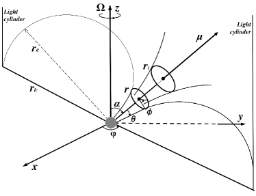
Figure 1: Geometry and parameters defined for an emitting beam. $\Omega$ indicates the rotation axis in $z$ direction, $\mu$ represents the magnetic axis, which is inclined by an angle of $\alpha$ with respect to $\Omega$. The LOF is tangential to the light cylinder, which has a polar angle $\theta$ from the magnetic axis $\mu$. The radiation beam has a radius of $\vartheta$ at a height of $r$.

Figure 2: Frequency dependence of the beam radius (FDB curve) calculated from the curvature radiation from particles of a single $\gamma$ for an inclined dipole of $\alpha=60^{\circ}$. Beam radii in the magnetic azimuth of $\phi=0^{\circ}$ and $\phi=90^{\circ}$ are frequency dependent, though the beam size of $\phi=0^{\circ}$ is smaller than that of $\phi=90^{\circ}$ at any frequency. This behavior is shown in the top panel for 300 MHz, 1.0 GHz and 2.0 GHz emission. The solid lines are calculated using two terms in Eq. (7), and the dashed lines are only for its first term. Here period $P=1$ s and $\gamma=400$ are taken for calculations.

The size and geometry of a dipole magnetic field is determined by pulsar period $P$, inclination angle $\alpha$ and impact angle $\beta$. In the polar coordinate system with the polar axis along the magnetic axis direction (Fig. 1), a dipole field-line can be described by $r=r_{e}~{}\sin^{2}\theta$, here $\theta$ is the polar angle from the magnetic axis, $r$ is the distance from the dipole origin, $r_{e}$ is the field-line constant, which is the distance from the origin to the point of the field-line intersection with the magnetic equatorial plane of $\theta=90\arcdeg$. For an inclined dipole, the LOF are contained in the light cylinder (see Fig. 1). The radius of the light-cylinder, $R_{\rm lc}=cP/2\pi$, gives the limit of the field line constants $r_{e}$ for the LOF, which is different for pulsars with different periods. The angular diameter of the polar cap defined by the feet of LOF on the neutron star surface is related to the pulsar period, $P$, by $2\theta_{\rm pc}=1.6\arcdeg P^{-1/2}$. The opening angle of the beam from the tangents of the LOF near the surface is about $1.2\arcdeg P^{-1/2}$, which defines the minimum geometrical beam angle. Observations show $\vartheta_{0}>1.2\arcdeg P^{-1/2}$. The emission beam determined by the LOF is not circular but compressed in the meridional direction in the plane of rotation and magnetic axes (Biggs, 1990). We define the magnetic azimuthal angle, $\phi$, starting from the connection between the magnetic axis and the rotation axis (to the top being the north) as being $\phi=0^{\circ}$ (see Fig. 2). The beam radius in the direction of $\phi=0^{\circ}$ is smaller than that in the direction of $\phi=90^{\circ}$ (to the east).

In the curvature radiation mechanism, the emission frequency is not only related to the field geometry but also to the Lorentz factor $\gamma$ of particles. The simplest case we consider here is that particles have the same Lorentz factor $\gamma$, and that the radio beam is defined by the tangents of the LOF. When a relativistic particle streams along a field-line, it can produce curvature radiation with a characteristic frequency of

$$\nu=\frac{3\gamma^{3}c}{4\pi\rho}.$$ (4)

Here, $\gamma$ is the Lorentz factor of particles in the range $10^{2}-10^{4}$, $\rho$ is the curvature radius of the particle trajectory. In any field-line, the curvature radius can be expressed by (Gangadhara, 2004)

$$\rho={r_{e}}\frac{\sin\theta(5+3\cos 2\theta)^{3/2}}{3\sqrt{2}(3+2\cos 2\theta)}.$$ (5)

Note that $\theta$ varies with $r$. The angle between the tangent of a field-line of $\theta$ and the magnetic axis is

$$\vartheta=\arccos(\frac{1+3\cos 2\theta}{\sqrt{10+6\cos 2\theta}}).$$ (6)

Combining Eq. (5) and Eq. (6), one can find the relation between $\vartheta$ and $\rho$ for any field-line of $r_{e}$. Because the radiation frequency $\nu$ is related to $\rho$ by Eq. (4), we get

$$\vartheta=15.4^{\circ}(\frac{\gamma^{3}c}{r_{e}\nu})+0.43^{\circ}(\frac{\gamma^{3}c}{r_{e}\nu})^{3}.$$ (7)

One can use Eq. (15) from Gangadhara (2004) to get the field-line constants $r_{e}$ for each LOF. Obviously, as indicated in Eq. (7), the beam radius is related to the radiation frequency. At a higher frequency of $\nu\gg\gamma^{3}c/r_{e}$, the second term can be neglected, and the beam radius $\vartheta$ is related to the frequency $\nu$ by roughly a power-law with the index of $k=-1$. At a low frequency of $\nu\leq\gamma^{3}c/r_{e}$, the frequency dependence becomes slightly steeper due to the contribution from the second term. Note that the beam radii in all magnetic azimuthal directions are frequency dependent. Clearly, the first term of Eq. (7) is a good approximation of the frequency dependence of pulsar beam, which has a power-law index $k=-1$.

Figure 3: Beam radii at a series of frequencies calculated from the curvature radiation of particles with a single $\gamma$. Default model parameters are $P=0.5$ s, $\alpha=60^{\circ}$, $\beta=0^{\circ}$ and $\gamma=400$. Various curves have been calculated for different parameters, $\alpha$, $\beta$, $P$ and $\gamma$ in four panels. Note that the two curves for $\alpha=60\arcdeg$ and $\alpha=30\arcdeg$ in the upper left panel are completely overlapped.

We calculated the beam radii at different frequencies for various model parameters, as shown in Fig. 3. All curves show the frequency dependence of radiation beam with a power-law index of approximately $-1$, which is different from observational values in the range of $-0.3>k>-1.2$ (Mitra & Rankin, 2002). We found that there is no influence on the frequency dependence of beam size by the magnetic inclination $\alpha$, because $\alpha$ only leads to the compression of beam in the meridional direction, and has almost no influence on the radius of $\phi=90^{\circ}$. Different impacts of line of sight with different $\beta$ values lead to different cuts of the beam from $\beta=0^{\circ}$ to $\beta=\vartheta$. The lower limit of $\vartheta$ is determined by the angular size of the polar cap (3/2$\theta_{\rm pc}$) or the $\beta$ value. Pulsars with a small period $P$ have a small $R_{\rm lc}$ and hence a small $r_{e}$ and a small curvature radius [Eq. (5)], which corresponds to a larger radiation frequency [Eq. (4)], as shown in Fig. 3. Note also that in the pulsar emission region curvature radiation of particles with a single $\gamma$ cannot produce radio emission over a wide frequency range from hundreds MHz to ten GHz. Particles with larger $\gamma$ produce curvature radiation at much higher frequency, which shifts the FDB curves to higher frequency ranges.

The calculations shown in Fig.2 and 3 were made with assumptions that pulsar beams are bounded by the LOF. However, Ruderman & Sutherland (1975) suggested that beam edge should be bounded by the critical field-lines, which are orthogonal to (instead of tangent to) the light cylinder at the intersection points. The critical field-lines are located between the magnetic axis and the LOF. Here, the parameter $\eta$ is used to describe the location of field-lines, with $\eta=0$ for the magnetic axis, $\eta=1$ for the LOF. To generate the curvature emission beam of the same open angle, the emission height from the critical field lines ($0<\eta<0.74$, depending on $\alpha$) is larger than that from the LOF as shown in Fig. 3, and the curvature radius is also larger, so that the emission has a smaller frequency of,

$$\nu=\nu_{\rm lof}\times\eta^{2}=\frac{3\gamma^{3}c}{4\pi\rho}\eta^{2},$$ (8)

with $\nu_{\rm lof}$ the corresponding emission frequency for the LOF. We carried out a set of calculations, and found that the curvature radiation for the critical field lines has almost the same frequency dependence of emission beam as that for the LOF, and $k$ and $\vartheta_{0}$ values are consistent within 5%, though $\nu_{0}$ is smaller due to larger curvature radii of field lines.

3 Curvature radiation beam from particles with various energy and density distributions

Particles in pulsar magnetosphere should have an energy distribution, which radiate in a range of frequencies at a range of heights for a given LOF. Furthermore, particles flow out along a set of open field-lines, rather than just the LOF. The pulsar radio emission from a given height and a given rotation phase is contributed from particles not only in the field lines which are tangential towards the observer, but also in the nearby field lines in the bunch within the $1/\gamma$ emission cone. The emission is coherent radiation from a bunch of particles (Buschauer & Benford, 1976).

According to simulation results of Medin & Lai (2010), we assume in this section that secondary particles for curvature radiation at radio bands follow a Gaussian energy distribution with a peak at $\gamma_{m}$ of several hundreds:

$$n_{\rm e}(\gamma)\sim\exp[-\frac{(\gamma-\gamma_{m})^{2}}{2\sigma_{\gamma}^{2}}].$$ (9)

Here, the standard deviation $\sigma_{\gamma}$ is of several tens. Considering the continuity of the particles flowing along the field-line tube, we got the number density of particles at $r$ as

$$n_{\rm e}(r)=n_{\rm e0}(r/R_{\star})^{-3}.$$ (10)

Here, $n_{\rm e0}$ represents the number density at the bottom of a magnetic field tube near the surface of a neutron star.

The power of curvature radiation at a frequency $\nu$ from one particle is given by,

$$P_{\rm e}=\frac{2q^{2}\gamma^{4}}{3c}(\frac{c}{\rho})^{2}.$$ (11)

$N_{b}$ particles in a field bunch in the region with a dimension size of less than half emission wavelength produce the total emission power of approximately $N_{b}^{2}\;P_{\rm e}$.

Because the curvature radius varies everywhere in the dipole field, according to Eq. (4) and (11), the observed emission at frequency $\nu$ and rotation phase $\varphi$ should come from the tangents of a set of open field-lines with the same magnetic azimuth $\phi$, where the curvature radius $\rho$ of a field-line and particle energy $\gamma$ are nicely combined to produce emission. The observed total power therefore should be the sum of them,

$$I(\nu,\varphi)=\int_{r_{\min}}^{r_{\max}}n_{\rm e}(r,\gamma)N_{b}^{2}P_{\rm e}(r,\phi,\gamma)dr.$$ (12)

Note that the magnetic azimuth $\phi$ is a monotonic function of the rotation phase $\varphi$, as given by Eq. (11) in Gangadhara (2004) which is equivalent to the well-known $S$-curve for polarization angle.

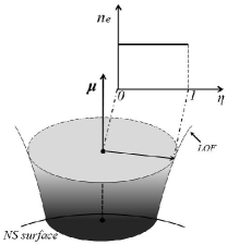
Figure 4: Illustration for the uniform density distribution of particles in pulsar magnetosphere. Here, $n_{\rm e}=n_{\rm e0}(r/R_{\star})^{-3}$.

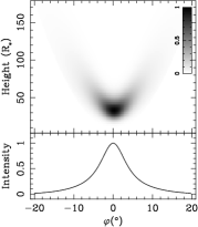
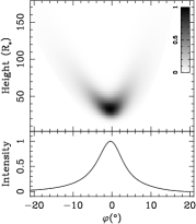
(a) without A&R effects	(b) with A&R effects

Figure 5: (a): Upper panel: Emission intensities at a given frequency (here $\nu=200$ MHz) for various rotation phases $\varphi$ and emission heights, radiated by a group of particles which have a Gaussian energy distribution and an uniform number distribution in magnetic polar angles as shown in Fig. 4. Lower panel: The accumulated emission profile (also at $\nu=200$ MHz). The model parameters used are $P=1$s, $\alpha=45^{\circ}$ and $\beta=3^{\circ}$, and $\gamma_{m}=350$ and $\sigma_{\gamma}=30$. (b): Same as left panels (a), but the abberation and retardation effects have been considered.

3.1 Emission beam from particles uniformly distributed in magnetic polar angles

As the first try, we assume that particles follow a Gaussian energy distribution and are uniformly distributed in the open field-lines for all magnetic polar angles, as shown in Fig. 4.

We can calculate the emission from each open field-line at every tangent for each frequency. At a given emission height, the central open field-lines have larger curvature radii than the outer open field-lines. Particles with a given Lorentz factor in the central field lines would produce a lower frequency emission [see Eq. (4)] than they do in the outer field lines. For a group of particles with a Gaussian energy distribution, only these particles with larger Lorentz factors in the central field lines can produce the emission at the same frequency as particles of lower Lorentz factors in the outer field lines, but their emission intensity is reduced by a factor of $1/\gamma^{2}$. Note that magnetic fields have smaller curvature radii at lower height. All these factors produce the bifurcation feature shown in Fig.5.

We limited our calculations for the region of $r_{\max}<0.1R_{\rm lc}$, because the emission intensity from higher regions is negligible (see Fig. 5) due to the relatively small particle density and large curvature radius. For $P=1$ s, $R_{\rm lc}\simeq 47771$ km $\simeq 4777R_{*}$, if we take $R_{*}=$10 km. We consider the phase shift (Gangadhara, 2005) of the emission from any height of every field-line, and integrate their emission for profiles at every observation frequency (lower panels in Fig. 5). We found that aberration and retardation effects can change the projection position of emission in the sky plane, which cause the profile to be enhanced by about 20% at the phase of $\varphi=-10^{\circ}$ and weakened by about 22% at the phase of $\varphi=10^{\circ}$ for the model calculations in Fig. 5.

We conclude that curvature radiation from particles uniformly distributed in magnetic polar angles cannot produce double conal profiles.

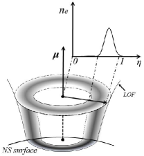
Figure 6: Illustration for the conal density distribution of particles in pulsar magnetosphere. The density follows Eq. (14).

3.2 Emission beam from particles in the conal density distribution

Small curvature radii of the magnetic field lines near the edge of the pulsar polar cap make curvature radiation more efficiently being generated, which then causes the sparkings more probably located around the edge of polar cap (Ruderman & Sutherland, 1975; Qiao et al., 2001). It is therefore possible that accelerated particles are more likely distributed in a conal area, instead of an uniform distribution. Noticed that charged particles flow out along a fixed line tube, we define the density distribution in a conal area on the polar cap as

$$n_{\rm e0}(\eta)=n_{\rm e0}{\exp}[-\frac{(\eta-\eta_{m})^{2}}{2\sigma_{\eta}^{2}}],$$ (13)

here $\eta_{m}$ denotes the peak position of the cone, and the standard derivation $\sigma_{\eta}$ describes the cone width. At any radius $r$ and any magnetic polar angle $\eta$ the density is

$$n_{\rm e}(r,\eta)=n_{\rm e0}(\eta)(r/R_{\star})^{-3},$$ (14)

which does not vary with magnetic azimuthal angle $\phi$. The illustration for the conal density distribution is given in Fig. 6.

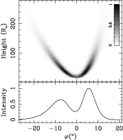
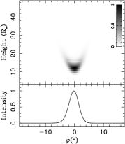
(a) $200$ MHz	(b) $800$ MHz

Figure 7: Same as Fig. 5 for emission intensity distributions and the accumulated profiles (a): at $200$ MHz and (b): at $800$ MHz for a conal density model. The particle energy and density distribution parameters are $\gamma_{m}=350$, $\sigma_{\gamma}=30$, $\eta_{m}=0.75$ and $\sigma_{\eta}=0.08$, with $P=1$s, $\alpha=45^{\circ}$ and $\beta=5^{\circ}$.

Figure 8: Integrated profiles at a series of frequencies calculated from curvature radiation of particles with a conal density distribution. The model parameters are the same as those in Fig. 7. The profiles are aligned to the absolute zero rotation phase when the sight line is in the meridional plane defined by the rotation and magnetic axes.

Similar to the uniform model in Sect.3.1, we calculated the curvature radiation of particles in such a density cone from each field line at every tangent at each frequency, to composite the emission beam between 100 MHz to 30 GHz. Fig. 7 shows the distribution of emission intensities for various heights and rotation phases as well as integrated profiles at two example frequencies, 200 MHz and 800 MHz. There are two components in the integrated profile at 200 MHz, though the emission for central rotation phases coming from the region of several tens of $R_{\star}$ is relatively strong compared to those from higher regions. The aberration and retardation effects, which shift high-altitude emission to early rotation phases, can cause the leading profile component to be wider and weaker than the trailing one at 200 MHz, as demonstrated by Dyks et al. (2010). At 800 MHz emission mostly comes from a lower region of about $r=10\sim 20R_{\star}$, rather than a few hundred of $R_{\star}$ for 200 MHz emission, where the sight line cuts only the beam edge and the emission from higher regions is too weak, so that only one component appears in the integrated profile. The profile evolves from two components at low frequencies to one component at frequencies of above 400 MHz (see Fig. 8).

Figure 9: Various FDB curves calculated from particles with a Gaussian energy distribution and a conal density distribution above the polar cap with different model parameters of $\alpha$, $\beta$, $\gamma_{m}$, $\sigma_{\gamma}$, $\eta_{m}$ and $\sigma_{\eta}$. The default parameters are the same as those in Fig. 7.

Table 2: Fitted parameters for various FDB curves in Fig. 9 from various conal density models with different parameters of $\alpha$, $\beta$, $\gamma_{m}$, $\sigma_{\gamma}$, $\eta_{m}$ and $\sigma_{\eta}$

$\alpha$	$\beta$	$\gamma_{m}$	$\sigma_{\gamma}$	$\eta_{m}$	$\sigma_{\eta}$	$\nu_{0}(\rm GHz)$	$k$	$\vartheta_{0}(^{\circ})$	$\vartheta_{\rm 100Mhz}(^{\circ})$
$20^{\circ}$	$3^{\circ}$	$350$	$30$	$0.75$	$0.08$	$1.35\pm 0.10$	$-1.24\pm 0.04$	$3.00$	$28.55\pm 0.38$
$45^{\circ}$	-	-	-	-	-	$1.15\pm 0.12$	$-1.18\pm 0.05$	$3.00$	$21.20\pm 0.39$
$70^{\circ}$	-	-	-	-	-	$0.75\pm 0.07$	$-1.18\pm 0.06$	$3.00$	$13.89\pm 0.26$
$45^{\circ}$	$1^{\circ}$	$350$	$30$	$0.75$	$0.08$	$1.93\pm 0.21$	$-1.01\pm 0.04$	$1.00$	$21.15\pm 0.40$
-	$3^{\circ}$	-	-	-	-	$1.15\pm 0.12$	$-1.18\pm 0.05$	$3.00$	$21.20\pm 0.39$
-	$5^{\circ}$	-	-	-	-	$0.84\pm 0.05$	$-1.31\pm 0.04$	$5.00$	$21.33\pm 0.24$
$45^{\circ}$	$3^{\circ}$	$300$	$30$	$0.75$	$0.08$	$0.57\pm 0.01$	$-1.35\pm 0.02$	$3.00$	$13.63\pm 0.07$
-	-	$350$	-	-	-	$1.15\pm 0.12$	$-1.18\pm 0.05$	$3.00$	$21.20\pm 0.39$
-	-	$400$	-	-	-	$2.23\pm 0.34$	$-1.07\pm 0.06$	$3.00$	$30.46\pm 0.72$
$45^{\circ}$	$3^{\circ}$	$350$	$10$	$0.75$	$0.08$	$1.12\pm 0.11$	$-1.30\pm 0.06$	$3.00$	$25.94\pm 0.56$
-	-	-	$30$	-	-	$1.15\pm 0.12$	$-1.18\pm 0.05$	$3.00$	$21.20\pm 0.39$
-	-	-	$50$	-	-	$1.06\pm 0.02$	$-0.96\pm 0.01$	$3.00$	$12.74\pm 0.05$
$45^{\circ}$	$3^{\circ}$	$350$	$30$	$0.60$	$0.08$	$0.65\pm 0.03$	$-1.27\pm 0.03$	$3.00$	$13.83\pm 0.13$
-	-	-	-	$0.75$	-	$1.15\pm 0.12$	$-1.18\pm 0.05$	$3.00$	$21.20\pm 0.39$
-	-	-	-	$0.90$	-	$1.74\pm 0.20$	$-1.15\pm 0.05$	$3.00$	$30.34\pm 0.58$
$45^{\circ}$	$3^{\circ}$	$350$	$30$	$0.75$	$0.06$	$1.12\pm 0.12$	$-1.19\pm 0.06$	$3.00$	$20.89\pm 0.41$
-	-	-	-	-	$0.08$	$1.15\pm 0.12$	$-1.18\pm 0.05$	$3.00$	$21.20\pm 0.39$
-	-	-	-	-	$0.10$	$1.17\pm 0.10$	$-1.19\pm 0.04$	$3.00$	$21.74\pm 0.34$

We measured the profile width at 10% of the peak intensity, and calculate the corresponding beam radius $\vartheta$ using Eq. (2). The FDB curves are plotted in Fig. 9 for various initial conditions. These curves are fitted using Eq. (3), and results are listed in Table 2. The profile width is close to zero when $\beta=\vartheta$. We have to fix $\vartheta_{0}$ to be the same as the impact angle $\beta$ during the fitting, because the emission at very high frequencies comes from the lowest emission point on the LOF. As seen in Fig. 9 and Table. 2, the FDB curves are closely related to emission geometry ($\alpha$, $\beta$), particle energy ($\gamma$, $\sigma_{\gamma}$) and conal density distributions ($\eta_{m}$).

We noticed that the FDB curves in all panels of Fig. 9 are converged to a similarly flattened FDB curve at high frequencies, except for various $\beta$ in panel b. As leaned from Fig. 7, the emission at high frequency comes from a very small height, so that the emission beam is rather narrow due to the geometrical effect. The density distribution ($\eta_{m}$, $\sigma_{\eta}$) and energy distribution ($\gamma$, $\sigma_{\gamma}$) of particles as well as the magnetic inclination ($\alpha$) do not have any obvious effect on the beam at high frequencies, as shown by the similarly converged flat FDB curves in all panels in Fig. 9. As expected, a sight line with a small impact angle $\beta$ can look into the much deeper magnetosphere and detect a much smaller beam at high frequencies (panel b in Fig. 9).

The FDB curves in Fig. 9 are influenced by $\alpha$, $\gamma$, $\sigma_{\gamma}$ and $\eta_{m}$ more obviously at the lower frequency end. For a larger magnetic inclination angle $\alpha$, the polar cap as well as pulsar beam will be more compressed in the meridian dimension (Fig. 2). When other model parameters are fixed, for a dipole field geometry with a larger $\alpha$, the fixed $\eta_{m}$ means that the bunch of field lines closer to the magnetic axis are used to calculate the emission beam, which have large curvature radii and emission frequencies are systematically smaller. The characteristic frequency $\nu_{0}$ of the FDB curves is therefore also smaller (see Table 2). Particles with a larger $\gamma_{m}$ produce emission of a given frequency at higher altitudes with larger curvature radii, which produce a wider beams (panel c in Fig. 9) with a large characteristic frequency $\nu_{0}$ (Table 2). If the energy distribution of particles is rather wide, e.g. for a model with a larger $\sigma_{\gamma}$, the emission region at a given frequency is very extended along field lines. However the dominant emission always comes from a lower emission height, and the integrated profile and hence the beam is much less sensitive to frequencies (panel d in Fig. 9). The particle distribution ($\eta_{m}$) is directly related to the field lines where the emission is produced. It is easy to understand that particle distributed with a small $\eta_{m}$ tends to emit with a smaller beam at any frequencies (panel e in Fig. 9). We noticed that the particle distribution width $\sigma_{\eta}$ does not have obvious influence on the FDB curves ( panel f in Fig. 9).

Figure 10: Distributions of $k$ and $\nu_{0}$ from 6375 combinations of various model parameter values of the conal density model.

(a) $k=-2.64$	(b) $k=-0.32$

Figure 11: Profile evolution with frequency for two extreme $k$ values: Panel (a) for an extreme steep frequency dependence of $k=-2.64$ with model parameters of $\alpha=45^{\circ}$, $\beta=9^{\circ}$, $\gamma_{m}=300$, $\sigma_{\gamma}=10$, $\eta_{m}=0.9$ and $\sigma_{\eta}=0.05$; and Panel (b) for an extreme flat frequency dependence of $k=-0.32$ with model parameters of $\alpha=65^{\circ}$, $\beta=1^{\circ}$, $\gamma_{m}=200$, $\sigma_{\gamma}=50$, $\eta_{m}=0.3$ and $\sigma_{\eta}=0.25$.

To further investigate the frequency dependence of pulsar beam radius on model parameters in a wide range of values, we have calculated the emission intensity distribution and integrated profiles (as shown in Fig. 7 and Fig. 8) for 6375 combinations of different parameter values: $\alpha=(5^{\circ}$, $25^{\circ}$, $45^{\circ}$, $65^{\circ}$, $85^{\circ}$), $\beta=(1^{\circ}$, $3^{\circ}$, $5^{\circ}$, $7^{\circ}$, $9^{\circ}$), $\gamma_{m}=(200$, $250$, $300$, $250$, $400$), $\sigma_{\gamma}=(10$, $30$, $50$), $\eta_{m}=(0.3$, $0.5$, $0.7$, $0.9$) and $\sigma_{\eta}=(0.05$, $0.1$, $0.15$, $0.2$, $0.25$). Pulsar period is fixed to be $P=1$s. The frequency dependence of beam radii are fitted with Eq. (3) to get $k$ and $\nu_{0}$. We got the distributions of $k$ and $\nu_{0}$ from these combinations as shown in Fig. 10. We found that values of $k$ are in the range of $-0.2$ to $-2.7$, consistent with observed values. However, profile components always merge to one component above $\sim 300MHz$, which is very different from observational facts of cone-dominant pulsars (Mitra & Rankin, 2002). We show in Fig. 11 the profile evolutions for two extremes of $k$ values: $k=-2.64$ and $k=-0.32$. For the case of $k=-0.32$, the two profile components merge even at a very low frequency below $100MHz$. The merging happens when $\gamma_{m}<250$ or $\sigma_{\gamma}>30$ or $\eta_{m}<0.5$ or $\sigma_{\eta}>0.15$. We noticed that when $\gamma_{m}>350$, for models of curvature radiation from particles in the conal density distribution, the emission below about $100MHz$ comes from the region of several thousands of $R_{\star}$, which leads profiles as wide as about $200^{\circ}$.

In summary, though curvature radiation models of particles in a conal density distribution can produce a proper range of $k$, the merging of profile components above few hundreds MHz is the main reason to reject the models for cone-dominated profiles.

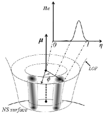
Figure 12: Illustration for the particle distribution in two density patches. The density follows Eq. (15).

3.3 Emission beam from particles of two density patches

In the inner gap model (Ruderman & Sutherland, 1975), the sparkings do not continually happen above the polar cap and are not concentrating in a ring area to produce the conal density distribution discussed above. The most probably case is that the sparkings occur separately above the polar cap, which produce the subbeams of the observed conal beam (Rankin, 1983) or the patchy beam (Lyne & Manchester, 1988; Han & Manchester, 2001). In the following we work on the models of curvature radiation of particles in two density patches which could be reasonably produced by two sparkings in the inner gap of a rotating neutron star.

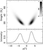
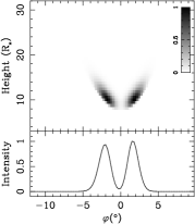
(a) $400$ MHz	(b) $1.6$ GHz

Figure 13: Same as Fig. 5 for emission intensity distributions and the accumulated profiles (a): at $400$ MHz and (b): at $1.6$ GHz for a model of two density patches. The particle energy and density distribution parameters are $\gamma_{m}=350$, $\sigma_{\gamma}=30$, $\eta_{m}=0.75$, $\sigma_{\eta}=0.08$, $\phi_{m}=45^{\circ}$ and $\sigma_{\phi}=12.5^{\circ}$, with $P=1$s, $\alpha=45^{\circ}$ and $\beta=3^{\circ}$.

Figure 14: Same as Fig. 8 except for the model of two density patches. The model parameters are the same as those in Fig. 13.

Table 3: Parameters fitted to the FDB curves in Fig. 15 for models of two density patches with various $\alpha$, $\beta$, $\gamma_{m}$, $\sigma_{\gamma}$, $\eta_{m}$, $\sigma_{\eta}$, $\phi_{m}$ and $\sigma_{\phi}$

$\alpha$	$\beta$	$\gamma_{m}$	$\sigma_{\gamma}$	$\eta_{m}$	$\sigma_{\eta}$	$\phi_{m}$	$\sigma_{\phi}$	$\nu_{0}(\rm GHz)$	$k$	$\vartheta_{0}(^{\circ})$	$\vartheta_{100}(^{\circ})$
$20^{\circ}$	$3^{\circ}$	$350$	$30$	$0.75$	$0.08$	$45^{\circ}$	$12.5^{\circ}$	$1.78\pm 0.11$	$-0.66\pm 0.02$	$3.00$	$9.71\pm 0.10$
$45^{\circ}$	-	-	-	-	-	-	-	$1.38\pm 0.04$	$-0.80\pm 0.01$	$3.00$	$11.17\pm 0.06$
$70^{\circ}$	-	-	-	-	-	-	-	$1.03\pm 0.03$	$-0.78\pm 0.01$	$3.00$	$9.24\pm 0.05$
$45^{\circ}$	$1^{\circ}$	$350$	$30$	$0.75$	$0.08$	$45^{\circ}$	$12.5^{\circ}$	$1.07\pm 0.05$	$-1.08\pm 0.02$	$1.00$	$13.84\pm 0.14$
-	$3^{\circ}$	-	-	-	-	-	-	$1.38\pm 0.04$	$-0.80\pm 0.01$	$3.00$	$11.17\pm 0.06$
-	$5^{\circ}$	-	-	-	-	-	-	$1.78\pm 0.13$	$-0.71\pm 0.02$	$5.00$	$12.65\pm 0.13$
$45^{\circ}$	$3^{\circ}$	$300$	$30$	$0.75$	$0.08$	$45^{\circ}$	$12.5^{\circ}$	$1.07\pm 0.05$	$-0.66\pm 0.02$	$3.00$	$7.78\pm 0.07$
-	-	$350$	-	-	-	-	-	$1.38\pm 0.04$	$-0.80\pm 0.01$	$3.00$	$11.17\pm 0.06$
-	-	$400$	-	-	-	-	-	$1.82\pm 0.04$	$-0.91\pm 0.01$	$3.00$	$16.99\pm 0.06$
$45^{\circ}$	$3^{\circ}$	$350$	$10$	$0.75$	$0.08$	$45^{\circ}$	$12.5^{\circ}$	$1.01\pm 0.06$	$-1.18\pm 0.03$	$3.00$	$18.49\pm 0.20$
-	-	-	$30$	-	-	-	-	$1.38\pm 0.04$	$-0.80\pm 0.01$	$3.00$	$11.17\pm 0.06$
-	-	-	$50$	-	-	-	-	$3.20\pm 0.69$	$-0.41\pm 0.03$	$3.00$	$7.08\pm 0.18$
$45^{\circ}$	$3^{\circ}$	$350$	$30$	$0.60$	$0.08$	$45^{\circ}$	$12.5^{\circ}$	$1.16\pm 0.05$	$-0.66\pm 0.01$	$3.00$	$8.01\pm 0.05$
-	-	-	-	$0.75$	-	-	-	$1.38\pm 0.04$	$-0.80\pm 0.01$	$3.00$	$11.17\pm 0.06$
-	-	-	-	$0.90$	-	-	-	$1.52\pm 0.03$	$-0.95\pm 0.01$	$3.00$	$16.26\pm 0.06$
$45^{\circ}$	$3^{\circ}$	$350$	$30$	$0.75$	$0.06$	$45^{\circ}$	$12.5^{\circ}$	$1.19\pm 0.04$	$-0.90\pm 0.01$	$3.00$	$12.24\pm 0.08$
-	-	-	-	-	$0.08$	-	-	$1.38\pm 0.04$	$-0.80\pm 0.01$	$3.00$	$11.17\pm 0.06$
-	-	-	-	-	$0.10$	-	-	$1.60\pm 0.08$	$-0.71\pm 0.02$	$3.00$	$10.17\pm 0.09$
$45^{\circ}$	$3^{\circ}$	$350$	$30$	$0.75$	$0.08$	$20^{\circ}$	$12.5^{\circ}$	$0.41\pm 0.02$	$-0.58\pm 0.03$	$3.00$	$5.35\pm 0.06$
-	-	-	-	-	-	$45^{\circ}$	-	$1.38\pm 0.04$	$-0.80\pm 0.01$	$3.00$	$11.17\pm 0.06$
-	-	-	-	-	-	$70^{\circ}$	-	$2.72\pm 0.09$	$-0.81\pm 0.01$	$3.00$	$17.41\pm 0.09$
$45^{\circ}$	$3^{\circ}$	$350$	$30$	$0.75$	$0.08$	$45^{\circ}$	$10.0^{\circ}$	$1.70\pm 0.12$	$-0.61\pm 0.02$	$3.00$	$8.58\pm 0.09$
-	-	-	-	-	-	-	$12.5^{\circ}$	$1.38\pm 0.04$	$-0.80\pm 0.01$	$3.00$	$11.17\pm 0.06$
-	-	-	-	-	-	-	$15.0^{\circ}$	$1.21\pm 0.03$	$-0.95\pm 0.01$	$3.00$	$13.67\pm 0.07$

The density distribution of two patches can be defined on the pulsar polar cap region and extended to high magnetosphere. For simplicity, we model two density patches (see Fig. 12) which are symmetrically located about the meridional plane and peaked at ($\eta_{m}$, $\phi_{m}$) and ($\eta_{m}$, $-\phi_{m}$), respectively, with Gaussian widths of $\sigma_{\eta}$ and $\sigma_{\phi}$ in the magnetic polar and azimuthal directions, i.e.

$$n_{\rm e}(r,\eta,\phi)=n_{e0}(r/R_{\star})^{-3}{\exp}[-\frac{(\eta-\eta_{m})^{2}}{2\sigma_{\eta}^{2}}]{\exp}[-\frac{(\phi\pm\phi_{m})^{2}}{2\sigma_{\phi}^{2}}].$$ (15)

The distribution of the emission intensity across height and the rotation phase and the evolution of integrated profiles with frequency for the curvature radiation model from particles of two density patches are shown in Fig. 13 and 14, respectively. Our model calculations show that: 1) the leading component is always slightly wider and weaker than the trailing one; 2) emission at a lower frequency comes from relatively higher and wider region ($10-50R_{\star}$ for $400$ MHz compared to $8-20R_{\star}$ for $1.6$ GHz); 3) the low-frequency profiles become wider and are shifted towards an early rotation phase; 4) the two components always remain resolved even at very high frequencies, because two density patches keep separated even down to the star surface.

Figure 15: Same as Fig. 9 but for the model for two density patches. The model parameters are the same as those in Fig. 13.

From simulated profiles at a set of frequencies, we calculated the beam radius and checked the frequency dependence of pulsar beam. We also checked if FDB curves are related to emission geometry ($\alpha$, $\beta$), particle energy distribution ($\gamma$, $\sigma_{\gamma}$) and patch geometry ($\eta_{m}$, $\sigma_{\eta}$, $\phi_{m}$ and $\sigma_{\phi}$). The curves are shown in Fig. 15 and fitted parameters are listed in Table 3. The influence of these parameters on the FDB curves are more or less similar to those found from the conal density models. We noticed that $\phi_{m}$ has the similar effect on the FDB curves as $\eta_{m}$, both of which determine the separation of the two patches. Particles in two patches with a larger $\sigma_{\phi}$ can produce the emission beams with a steeper FDB curve.

Figure 16: Distributions of $k$ and $\nu_{0}$ from 29070 combinations of various model parameter values of the two density patch model.

(a) $k=-2.02$	(b) $k=-0.09$

Figure 17: Profile evolutions with frequency in the two density patch model for two extreme values of $k$, Panel (a) for $k=-2.02$ and Panel (b) for $k=-0.09$. Model parameters for panel (a) are $\alpha=45^{\circ}$, $\beta=5^{\circ}$, $\gamma_{m}=400$, $\sigma_{\gamma}=10$, $\eta_{m}=0.9$, $\sigma_{\eta}=0.1$, $\phi_{m}=65^{\circ}$ and $\sigma_{\phi}=15^{\circ}$, and for panel (b) are $\alpha=45^{\circ}$, $\beta=1^{\circ}$, $\gamma_{m}=200$, $\sigma_{\gamma}=90$, $\eta_{m}=0.3$, $\sigma_{\eta}=0.05$, $\phi_{m}=45^{\circ}$ and $\sigma_{\phi}=5^{\circ}$.

To investigate the possible range of $k$ and $\nu_{0}$ in the two density patch model, we have calculated the integrated profiles and fitted the FDB curves for 29070 sets of models with different combinations of model parameters of $\alpha=(5^{\circ}$, $45^{\circ}$, $85^{\circ}$), $\beta=(1^{\circ}$, $5^{\circ}$, $9^{\circ}$), $\gamma_{m}=(200$, $300$, $400$), $\sigma_{\gamma}=(10$, $50$, $90$), $\eta_{m}=(0.1$, $0.3$, $0.5$, $0.7$, $0.9$), $\sigma_{\eta}=(0.05$, $0.1$, $0.15$, $0.2$, $0.25$), $\phi_{m}=(25^{\circ}$, $45^{\circ}$, $65^{\circ}$, $85^{\circ}$) and $\sigma_{\phi}=(5^{\circ}$, $15^{\circ}$, $25^{\circ}$, $35^{\circ}$, $45^{\circ}$). The distributions of the power-law indices $k$ and the characteristic frequency $\nu_{0}$ are shown in Fig. 16. We noticed that $k$ values are in the range between $-0.1$ and $-2.5$. Two components are always resolved, except for the extreme case shown in Fig. 17(a) in which emission is radiated by particles with a narrower energy distribution ($\sigma_{\gamma}=10$) and peaking at a larger energy ($\gamma_{m}=400$) at very high $\eta_{m}=0.9$ and $\phi_{m}=65$.

Figure 18: Beam radii ($\vartheta_{10}$) calculated from the 10% profile widths ($W_{10}$) at a series of frequencies are compared with beam radii ($\vartheta_{50}$) calculated from the 50% profile widths ($W_{50}$) and beam radii ($\vartheta_{pp}$) calculated from component separations ($W_{pp}$). Parameters for this example model are $\gamma_{m}=200$, $\sigma_{\gamma}=50$, $\eta_{m}=0.7$, $\sigma_{\eta}=0.2$, $\phi_{m}=65^{\circ}$ and $\sigma_{\phi}=15^{\circ}$, with $P=1s$, $\alpha=45^{\circ}$ and $\beta=5^{\circ}$.

Figure 19: Comparison of $k$ and $\nu_{0}$ values calculated from $\vartheta_{10}$ and $\vartheta_{pp}$

In above beam calculations, we used the profile width $W_{10}$ at 10% of pulse peak. If the separations $W_{pp}$ of two components are used to calculated the beam radii, the beam sizes are obviously smaller than those calculated from the 50% and 10% widths (Fig. 18). We compared in Fig. 19 the $k$ and $\nu_{0}$ values calculated from $\vartheta_{10}$ (written as $k_{10}$ and $\nu_{0,10}$) with the $k$ and $\nu_{0}$ values from $\vartheta_{pp}$ (written as $k_{pp}$ and $\nu_{0,pp}$), and found that they are correlated and scatter at small $\nu_{0}$ or large $k$ values (due to error-bar as expected).

In summary, the curvature radiation from particles in two density patches can not only give a proper range of $k$ values, but also keeps the two components resolved in general even at very high frequencies.

4 Discussions

In the previous section, we conclude that the FDB curves with two resolved components can be preferably explained by curvature radiations of particles in two density patches. Here we discuss influences on the FDB curves by the radial decay of particle energy and by other possible energy distribution of particles, and discuss the possible FDB curve flattening at low frequencies. Finally we will look at the real FDB data and make a model.

4.1 Radial decay of particle energy and the lowest emission height

As shown in Fig. 9 and 15, the values of beam radii at the infinite-frequency, $\vartheta_{0}$, calculated from models are always very close to those of $\beta$, no matter what model parameters are in putted. However, both on observational ground (Table. 1) and theoretical expectations, $\vartheta_{0}$ is larger than $\beta$.

In simulations above we assume that particles in the magnetosphere have a Gaussian energy distribution with a peak Lorentz factor $\gamma_{m}$ and a spread width $\sigma_{\gamma}$ along the whole trajectory. In reality, the particle energy distribution may be much more complicated due to the Compton loss (Zhang et al., 1997) or other processes. It is reasonable to believe that particle energy decreases when they flow out along the field lines in the inner magnetosphere.

In the vacuum-gap model (Ruderman & Sutherland, 1975), electron-positron pairs are produced by the avalanche process in the pulsar polar cap. The maximum Lorentz factor of the primary particles after accelerating across the gap is $\gamma_{\max}=1.2\times 10^{7}B_{\star 12}h_{4}^{2}/P_{\rm 1s}$, with $B_{\star 12}=B_{\star}/10^{12}$ G the surface magnetic field, $h_{4}=h/10^{4}\,$cm the gap height and $P_{\rm 1s}=P/{\rm 1s}$. Pair cascade occurs within a few stellar radii near the surface, which generates the secondary particles with much lower Lorentz factors of a few hundred. Detailed numerical simulations on the pair cascade process were carried out by Medin & Lai (2010), in which they found that for various initial parameters (such as surface magnetic field, period and primary energy), the pair cascade process maybe finishes at a height of several star-radius, from less than $2R_{\star}$ to more than $10R_{\star}$. Here we naively assume a toy model to describe the rapid decay of particle energy during the pair cascade process, which reads

$$\gamma_{m}=\gamma_{m0}\exp(-q\frac{r-R_{\star}}{R_{\star}})+\gamma_{s},$$ (16)

here $\gamma_{m}$ is the peak Lorentz factor of the Gaussian distribution we used above, $\gamma_{m0}$ and $\gamma_{s}$ are the corresponding values of the primary particles and the final secondary particles before and after the pair cascade, respectively. The factor $q$ (less than 1) determines how fast the energy decreases with height for the cascade. This energy model has been used by Qiao et al. (2001) and Zhang et al. (2007) to simulate the inverse-Compton scattering emission, where they ignored the energy term $\gamma_{s}$. To use the above energy model in our simulation for the model for two density patches, one should substitute $\gamma_{m}$ of Eq. (16) into the Gaussian energy distribution Eq. (9). Note that the number of the particles $n_{\rm e0}$ in Eq. (15) should also be replaced by $n_{\rm e0}\gamma_{s}/\gamma_{m}$ to keep the conservation of total energy.

Figure 20: FDB curves for the curvature radiation model by particles in two density patches with an energy distribution of Eq. (9) and Eq. (16). The default model parameters are the same as those in Fig 13 (e.g. $\beta=3^{\circ}$) but also with $\gamma_{m0}=10^{6}$, $q=0.3$ and $\gamma_{s}=350$.

Table 4: Fitted parameters of FDB curves in Fig. 20

$\gamma_{m0}$	$q$	$\gamma_{s}$	$\nu_{0}(\rm GHz)$	$k$	$\vartheta_{0}(^{\circ})$
$10^{5}$	$0.3$	$350$	$0.84\pm 0.05$	$-0.91\pm 0.03$	$4.39\pm 0.05$
$10^{6}$	-	-	$0.72\pm 0.05$	$-0.93\pm 0.03$	$5.11\pm 0.05$
$10^{7}$	-	-	$0.64\pm 0.05$	$-0.94\pm 0.04$	$5.76\pm 0.05$
$10^{6}$	$0.2$	$350$	$0.82\pm 0.06$	$-0.84\pm 0.03$	$6.07\pm 0.05$
-	$0.3$	-	$0.72\pm 0.05$	$-0.93\pm 0.03$	$5.11\pm 0.05$
-	$0.5$	-	$0.72\pm 0.03$	$-0.99\pm 0.02$	$4.18\pm 0.03$
$10^{6}$	$0.3$	$250$	$0.35\pm 0.04$	$-0.71\pm 0.06$	$5.06\pm 0.05$
-	-	$350$	$0.72\pm 0.05$	$-0.93\pm 0.03$	$5.11\pm 0.05$
-	-	$450$	$1.85\pm 0.30$	$-0.99\pm 0.06$	$4.93\pm 0.22$

Example FDB curves from the curvature radiation model by particles in two density patches with an energy distribution described by Eq. (9) and Eq. (16) are demonstrated in Fig. 20, and the fitted parameters are listed in Table. 4. We found that a larger primary Lorentz factor $\gamma_{m0}$ or a smaller $q$ lead to larger beam radius $\vartheta_{0}$ at very high frequencies. A larger $\gamma_{s}$ leads to a steeper FDB curve.

In these model the values of $\vartheta_{0}$ are always larger than those of $\beta$, which means that there exists the lowest radio emission height $r_{\rm low}=R_{\rm lc}\sin^{2}(2\vartheta_{0}/3)$, which is $>R_{\rm lc}\sin^{2}(2\beta/3)$. For a small value of $\vartheta_{0}$, the corresponding beam radii at the infinite frequency can be written as $\vartheta_{0}\simeq 3/2\sqrt{r_{\rm low}/R_{\rm lc}}$. Now, what is the value of $r_{\rm low}$?

Figure 21: Characteristic Lorentz factor $\gamma_{c}$ at lowest radio emission height well related to $\gamma_{m0}$ and $q$. Symbols $*$ come from simulation data as in Table 4 and lines are the fitting.

According to Eq. (16), at the lowest radio emission height $r_{\rm low}$, there exists a characteristic Lorentz factor $\gamma_{c}$. We noticed that $r_{\rm low}$ and $\gamma_{c}$ are related with $\gamma_{m0}$ and $q$ by:

$$\frac{r_{\rm low}}{R_{\star}}=1-\frac{1}{q}\ln\frac{\gamma_{c}}{\gamma_{m0}}.$$ (17)

From simulations similarly as presented Table 4, we can get a set of $r_{\rm low}$ from $\vartheta_{0}$ for various $\gamma_{m0}$ and $q$, and then we got $\gamma_{c}$ using Eq. (17). We find that $\gamma_{c}$ are also very well related to $\gamma_{m0}$ and $q$, as shown in Fig. 21, by

$$\gamma_{c}=55.0\gamma_{m0}^{0.4}\exp{(-2q)}.$$ (18)

Substituting into Eq. (17), we find

$${r_{\rm low}}={R_{\star}}(3+\frac{1.38\log\gamma_{m0}-4}{q}).$$ (19)

Figure 22: Same as Fig. 14 but a power-law energy distribution with index $s=-2$. Other model parameters are $\gamma_{s,\rm min}=150$ and $\gamma_{s,\rm max}=2000$, $\gamma_{m}=350$, $\sigma_{\gamma}=30$, $\eta_{m}=0.75$, $\sigma_{\eta}=0.08$, $\phi_{m}=45^{\circ}$ and $\sigma_{\phi}=12.5^{\circ}$, with $P=1$s, $\alpha=45^{\circ}$ and $\beta=3^{\circ}$.

4.2 On the energy distribution of particles

At any height, the secondary particles in the magnetosphere for the curvature radio emission were assumed to have an energy distribution in the Gaussian function. It is possible that the particles follow other energy distribution functions. For example, according to Arons (1981), the multi-component plasma in pulsar magnetosphere contains secondary pairs, a high-energy plasma ‘tail’, and some primary particles. The joint energy distribution of secondary particles and high-energy ‘tail’ can be described by a power-law with two cutoffs at its two ends, which reads as,

$$n_{\rm e}(\gamma)\sim\gamma^{s},\,\,\,\,\gamma_{s,\rm min}<\gamma<\gamma_{s,\rm max},$$ (20)

where $s$ is the power-law index. The curvature radiation from particles in two density patches with such an energy distribution produces the integrated profiles at a series of frequencies with a similar shape and a constant pulse width between 80 MHz and 40 GHz, as shown in Fig. 22. We can not find the profile differences for a range of $s$ values, e.g. a difference less than $2\%$ for the pulse width values between $s=-2$ and $s=-3$. We also found that the values of $\gamma_{s,\rm min}$ and $\gamma_{s,\rm max}$ determine the frequency range for the constant profile width.

Figure 23: Example of Low frequency flattening the FDB curve. The model parameters are $\gamma_{m}=400$, $\sigma_{\gamma}=10$, $\eta_{m}=0.7$, $\sigma_{\eta}=0.1$, $\phi_{m}=45^{\circ}$ and $\sigma_{\phi}=5^{\circ}$ with $P=1s$, $\alpha=45^{\circ}$ and $\beta=5^{\circ}$.

4.3 Possible low frequency flattening of the FDB curves

During the model calculations, we noticed that the FDB curves tend to be flattening at low frequencies. For some input parameters of the two density patch model, the effect is very obvious (Fig. 23), especially when Lorentz factors are large ($\gamma_{m}>400$) and/or the energy distribution is broad ($\sigma_{\gamma}>80$).

This is understandable. Because of the dipole bending of magnetic field lines, as pulsar rotates, a fixed sight-line cut across the two density patches (see Fig. 12) with a clear lower limit and upper limit of height and a clear left and right limit of the rotation phase. Very low frequency emissions tend to come from the high regions of two patches in such a limited volume. In that high regions near the upper bound, the lower frequency emission comes from particles of the lower energy, but the pulse-width or beam-width of the emission from two patches is determined by the geometry. This happens to very low-frequency, depending on the $\gamma_{m}$. The low-frequency flattening of FDB curves are often seen in the models when patches are small (small $\sigma_{\phi}$), or energy of particles are very high and/or the energy distribution is broad (large $\gamma_{m}$ and $\sigma_{\gamma}$).

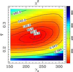
Figure 24: Upper panel: An example of real data and model-fitting. The observed data of PSR B2020+28 are taken from Mitra & Rankin (2002). The solid line is the best model calculated from the curvature radiation of particles in two density patches with parameters $\gamma_{m0}=10^{6}$, $\gamma_{s}=225$, $\sigma_{\gamma}=15$, $q=0.25$, $\eta_{m}=0.75$, $\sigma_{\eta}=0.08$, $\phi_{m}=45^{\circ}$ and $\sigma_{\phi}=12.5^{\circ}$. The geometrical parameters $\alpha$ and $\beta$ and the period of this pulsar can be found from Table 1. Lower panel: The $\chi^{2}$ distribution for a pair of the most influential parameters, $\gamma_{s}$ and $q$, for the fitting. The best values are $\gamma_{s}=225$ and $q=0.25$.

4.4 Observed FDB curve and a model

We have worked on a huge number of models for the radio emission intensity distribution across the height and rotation phase and integrated profiles. We now look at data of a real cone-dominant pulsar, PSR B2020+28, and make a model. The data are taken from (Mitra & Rankin, 2002). To keep the two profile components separated even at very high frequencies, we have to choose a model of the curvature radiations of particles in two density patches and consider the energy distribution of particles as described by Eq. (9) and Eq. (16). As shown in Figure 24, the model can fit data nicely with a local minimum of $\chi^{2}=10.24$ in the parameter space of $\gamma_{s}$ and $q$. The model is obtained with sparsely separated parameter grids, which may be improved by a global fitting for 8 parameters but that is very computational expensive.

5 Summary and outlook

We studied the frequency dependence of beam radius for cone-dominant pulsars by using the curvature radiation mechanism.

For the simplest case in which pulsar radio emission is generated by curvature radiation of relativistic particles with a single $\gamma$ and streaming along fixed open field-lines, we obtain the analytic formula in Eq. (7) for the frequency dependence. It has the power-law index $k=-1$, and $\vartheta_{0}=0$, both are different from observations.

Considering various density distribution and energy distribution of particles, we numerically calculated the intensity of curvature radiation from all the possible emission heights in the open field line region, and get integrated mean pulse profiles from which the FDB curves are derived. We found that the power-law index $k$ and $\vartheta_{0}$ are strongly influenced by the density distribution and energy distribution of particles in the open field-line region.

When particles are uniformly distributed in whole open field lines, the curvature radiation can produce only one profile component, which can not explain the two resolved components of cone-dominant pulsars.

When particles are distributed in a conal area, the low-frequency emission comes from very high regions so that profile is very wide. Profiles at high frequencies cannot have two separated components, because emission comes from low heights where the sight line always continually cuts the edge of density cone.

To keep two profile components separated or resolved, the particles must come from two density patches. Model calculations from a huge amount of parameter combinations show that the $k$ values of the FDB curves are in the range of $-0.1$ to $-2.5$, in agreement with the observations. Because of the limited upper boundary of the density patches cut by a given sight line, the FDB curves tends to be flattened at low frequencies, especially for models with a large Lorentz factor and/or broad particle energy distribution.

The geometry of density distribution of particles and the energy distribution of particles in the model certainly affect the FDB curves. For a Gaussian energy distribution, high energy particles with large $\gamma_{m}$ will produce a wide beam at low frequency. Particles in a narrow energy distribution with a small $\sigma_{\gamma}$ produce a steep FDB curve. The radial decay of particle energy is important to get a reasonable $\vartheta_{0}$ in models.

Through model calculations of pulsar beam and profile evolution by using the curvature radiation mechanism, we have clarified some important issues on particle density and energy distributions. However, in our simulations, we considered only the simple case that particles are emitting radio waves with the characteristic frequency for curvature radiation determined by the Lorentz factor. The real curvature emission of any particles has an energy spectrum, which is a power-law with an index $1/3$ at the low frequency limit (much less than the characteristic frequency) and becomes exponential at high frequencies. This may significantly affect the emission regions and modify the FDB curves, which we should investigate in future. Another important fact is that the real pulsar radio emission is believed to be highly coherent, while in this paper we simply treat the coherence by assuming that the emission comes from point-like huge charge. Moreover, other emission mechanisms may also work in pulsar magnetosphere, such as inverse Compton scattering, plasma oscillation, cyclotron instability and Coulomb bremsstrahlung emission, etc, which are not considered in this paper and may lead to their own FDB curves.

References

- Arons (1981) Arons, J. 1981, in ESA Special Publication, Vol. 161, ESA Special Publication, ed. T. D. Guyenne & G. Lévy, 273
- Beskin et al. (1988) Beskin, V. S., Gurevich, A. V., & Istomin, Y. N. 1988, Ap&SS, 146, 205
- Biggs (1990) Biggs, J. D. 1990, MNRAS, 245, 514
- Buschauer & Benford (1976) Buschauer, R. & Benford, G. 1976, MNRAS, 177, 109
- Cordes (1978) Cordes, J. M. 1978, ApJ, 222, 1006
- Dyks & Harding (2004) Dyks, J. & Harding, A. K. 2004, ApJ, 614, 869
- Dyks et al. (2010) Dyks, J., Wright, G. A. E., & Demorest, P. 2010, MNRAS, 405, 509
- Everett & Weisberg (2001) Everett, J. E. & Weisberg, J. M. 2001, ApJ, 553, 341
- Gangadhara (2004) Gangadhara, R. T. 2004, ApJ, 609, 335
- Gangadhara (2005) Gangadhara, R. T. 2005, ApJ, 628, 923
- Gil (1981) Gil, J. 1981, Acta Phys. Pol., B12, 1081
- Han & Manchester (2001) Han, J. L. & Manchester, R. N. 2001, MNRAS, 320, L35
- Lyne & Manchester (1988) Lyne, A. G. & Manchester, R. N. 1988, MNRAS, 234, 477
- Machabeli & Usov (1989) Machabeli, G. Z. & Usov, V. V. 1989, Sov. Astron. Lett., 15, 393
- Manchester (1995) Manchester, R. N. 1995, J. Astrophys. Astr., 16, 107
- Medin & Lai (2010) Medin, Z. & Lai, D. 2010, MNRAS, 406, 1379
- Mitra & Rankin (2002) Mitra, D. & Rankin, J. M. 2002, ApJ, 577, 322
- Phillips (1992) Phillips, J. A. 1992, ApJ, 385, 282
- Qiao et al. (2001) Qiao, G. J., Liu, J. F., Zhang, B., & Han, J. L. 2001, A&A, 377, 964
- Rankin (1983) Rankin, J. M. 1983, ApJ, 274, 333
- Rankin (1990) Rankin, J. M. 1990, ApJ, 352, 247
- Ruderman & Sutherland (1975) Ruderman, M. A. & Sutherland, P. G. 1975, ApJ, 196, 51
- Thorsett (1991) Thorsett, S. E. 1991, ApJ, 377, 263
- Vitarmo & Jauho (1973) Vitarmo, J. & Jauho, P. 1973, ApJ, 182, 935
- Xilouris et al. (1996) Xilouris, K. M., Kramer, M., Jessner, A., Wielebinski, R., & Timofeev, M. 1996, A&A, 309, 481
- Zhang et al. (1997) Zhang, B., Qiao, G. J., & Han, J. L. 1997, ApJ, 491, 891
- Zhang et al. (2007) Zhang, H., Qiao, G. J., Han, J. L., Lee, K. J., & Wang, H. G. 2007, A&A, 465, 525