Kernelet: High-Throughput GPU Kernel Executions with Dynamic Slicing and Scheduling

Abstract

Graphics processors, or GPUs, have recently been widely used as accelerators in the shared environments such as clusters and clouds. In such shared environments, many kernels are submitted to GPUs from different users, and throughput is an important metric for performance and total ownership cost. Despite the recently improved runtime support for concurrent GPU kernel executions, the GPU can be severely underutilized, resulting in suboptimal throughput. In this paper, we propose Kernelet, a runtime system with dynamic slicing and scheduling techniques to improve the throughput of concurrent kernel executions on the GPU. With slicing, Kernelet divides a GPU kernel into multiple sub-kernels (namely slices). Each slice has tunable occupancy to allow co-scheduling with other slices and to fully utilize the GPU resources. We develop a novel and effective Markov chain based performance model to guide the scheduling decision. Our experimental results demonstrate up to 31.1% and 23.4% performance improvement on NVIDIA Tesla C2050 and GTX680 GPUs, respectively.

1 Introduction

The graphics processing unit (or GPU) has become an effective accelerator for a wide range of applications from computation-intensive applications (e.g.,  [43, 25, 26]) to data-intensive applications (e.g,  [10, 18]). Compared with multicore CPUs, new-generation GPUs can have much higher computation power in terms of FLOPS and memory bandwidth. For example, an NVIDIA Tesla C2050 GPU can deliver the peak single precision floating point performance of over one Tera FLOPS, and memory bandwidth of 144 GB/s. Due to their immense computation power and memory bandwidth, GPUs have been integrated into clusters and cloud computing infrastructures. In Top500 list of November 2012, two out of the top ten supercomputers are with GPUs integrated. Amazon and Penguin have provided virtual machines with GPUs. In both cluster and cloud environments, GPUs are often shared by many concurrent GPU programs (or kernels) (most likely submitted by multiple users). Additionally, to enable sharing GPUs remotely, a number of software frameworks such as rCUDA [7] and V-GPU [45] have been developed. This paper studies whether and how we can improve the throughput of concurrent kernel executions on the GPU.

Throughput is an important optimization metric for efficiency and the total ownership cost of GPUs in such shared environments. First, many GPGPU applications such as scientific and financial computing tasks are usually throughput oriented [9]. A high throughput leads to the high performance and productivity for users. Second, compared with CPUs, GPUs are still expensive devices. Therefore, a high throughput not only means a high utilization on GPU resources but also the total ownership cost of running the application on the GPU. That might also be one of the reasons that GPUs are usually deployed and shared to handle many kernels from users.

Recently, we have witnessed the success of GPGPU research. However, most studies focus on single-kernel optimizations (e.g., new data structures [17] and GPU friendly computing patterns [10, 11]). Despite the fruitful research, a single kernel usually severely under-utilizes the GPU. This severe underutilization is mainly due to the inherent memory and computation behavior of a single kernel (e.g., irregular memory accesses and execution pipeline stalls). In our experiments, we have studied eight common kernels (details are presented in Section 5). On C2050, their average $\mathit{IPC}$ is 0.52, which is far from the optimal value (1.0). Their memory bandwidth utilization is only ranging from 0.02% to 14%.

Recent GPU architectures like NVIDIA Fermi [27] architecture supports concurrent kernel executions, which allows multiple kernels to be executed on the GPU simultaneously if resources are allowed. In particular, Fermi adopts a form of cooperative kernel scheduling. Other kernels requesting the GPU must wait until the kernel occupying the GPU voluntarily yields control. Here, we use NVIDIA CUDA’s terminology, simply because CUDA is nowadays widely adopted in GPGPU applications. A kernel consists of multiple executions of thread blocks with the same program on different data, where the execution order of thread blocks is not defined. On the Fermi GPUs, one kernel can take the entire GPU as long as it has sufficient thread blocks to occupy all the multi-processors (even though it can have severely low resource utilization). Concurrent execution of two such kernels almost degrades to sequential execution on individual kernels. Recent studies [34] on scheduling the concurrent kernels mainly focus on the kernels with low occupancy (i.e., the thread blocks of a single kernel cannot fully utilize all GPU multiprocessors). However, the occupancy of kernels (with large input data sizes in practice) is usually high after single-kernel optimizations.

Individual kernels as a whole cannot realize the real sharing of the GPU resources. A natural question is: can we slice the kernel into small pieces and then co-schedule slices from different kernels in order to improve the GPU resource utilization? The answer is yes. One observation is that GPU kernels (e.g., those written in CUDA or OpenCL) conform to the SPMD (Single Program Multiple Data) execution model. In such data-parallel executions, a kernel execution can usually be divided into multiple slices, each consisting of multiple thread blocks. Slices can be viewed as low-occupancy kernels and can be executed simultaneously with slices from other kernels. The GPGPU concurrent kernel scheduling problem is thus converted to the slice scheduling problem.

With slicing, we have two more issues to address. The first issue is on the slicing itself: what is the suitable slice size? How to perform the slicing in a transparent manner? The smallest granularity of a slice is one thread block, which can lead to significant runtime overhead of submitting too many such small slices onto the GPUs for execution. To the other extreme, the largest granularity of the slice is the entire kernel, which degrades to the non-sliced execution. The second issue is how to select the slices for co-schedule in order to maximize the GPU utilization.

To address those issues, we develop Kernelet, a runtime system with dynamic slicing and scheduling techniques to improve the GPU utilization. Targeting at the concurrent kernel executions in the shared GPU environment, Kernelet dynamically performs slicing on the kernels, and the slices are carefully designed with tunable occupancy to allow slices from other kernels to utilize the GPU resources in a complementary way. For example, one slice utilizes the computation units and the other one on memory bandwidth. We develop a novel and effective Markov chain based performance model to guide kernel slicing and scheduling in order to maximize the GPU resource utilization. Compared with existing GPU performance models which are limited to a single kernel only, our model are designed to handle heterogeneous workloads (i.e., slices from different kernels). We further develop a greedy co-scheduling algorithm to always co-schedule the slices from the two kernels with the highest performance gain according to our performance model.

We have evaluated Kernelet on two latest GPU architectures (Tesla C2050 and GTX680). The GPU kernels under study have different memory and computational characteristics. Experimental results show that 1) our analytical model can accurately capture the performance of heterogeneous workloads on the GPU, 2) our scheduling increase the GPU throughput by up to 31.1% and 23.4% on C2050 and GTX680, respectively.

Organization. The rest of the paper is organized as follows. We introduce the background and definition of our problem in Section 2. Section 3 presents the system overview, followed by detailed design and implementation in Section 4. The experimental results are presented in Section 5. We review the related work in Section 6 and conclude this paper in Section 7.

2 Background and Problem Definition

In this section, we briefly introduce the background on GPU architectures, and next present our problem definition.

2.1 GPU Architectures

GPUs have rapidly evolved into a powerful accelerator for many applications, especially after CUDA was released by NVIDIA [30]. The top tags in http://gpgpu.org/ show that a wide range of applications have been accelerated with GPGPU techniques, including vision and graphics, image processing, linear algebra, molecular dynamics, physics simulation and scientific computing etc. Those applications cover quite a wide range of computation and memory intensiveness. In the shared environment like clusters and cloud, it is very likely that users submit kernels from different applications to the same GPU. Thus, it is feasible to schedule kernels with different memory and computation characteristics to better utilize GPU resources.

This paper focuses on the design and implementation with NVIDIA CUDA. Since OpenCL and CUDA have very similar designs, our design and implementation can be extended to OpenCL with little modification. Kernelet takes advantage of concurrent kernel execution capability of new-generation GPUs like NVIDIA Fermi GPUs. With the introduction of CUDA, a GPU can be viewed as a many-core processor with a set of streaming multi-processors (SM). Each SM has a set of scalar cores, which executes the instructions in the SIMD (Single Instruction Multiple Data) manner. The SMs are in turn executed in the SPMD manner. The program is called kernel.

In CUDA’s abstraction, GPU threads are organized in a hierarchical configuration: usually 32 threads are firstly grouped into a warp; warps are further grouped into thread blocks. The CUDA runtime performs mapping and scheduling at the granularity of thread blocks. Each thread block is mapped and scheduled on an SM, and cannot be split among multiple SMs. Once a thread block is scheduled, its warps become active on the SM. Warp is the smallest scheduling unit on the GPU. Each SM uses one or more warp schedulers to issue instructions of the active warps. Another important resource of the GPU is shared memory, which is a small piece of scratchpad memory at the scope of a thread block. It is small and has very low latency. Shared memory is visible for all the threads in the same thread block.

We define the SM occupancy as the ratio of active warps to the maximum active warps that are allowed to run on the SM. Higher occupancy means higher thread parallelism. The aggregated register and shared memory usage of all warps should not exceed the total amount of available registers and shared memory on an SM.

Block Scheduling. CUDA runtime system maps thread blocks to SMs in a round-robin manner. If the number of thread blocks in a kernel is less than the number of SMs on the GPU, each thread block will be executed on a dedicated SM; otherwise, multiple thread blocks will be mapped to the same SM. The number of thread blocks that can be concurrently executed on the SM depends on their total resource requirements (in terms of registers and shared memory). If the kernel currently being executed on the GPU cannot fully utilize the GPU, the GPU allows to schedule thread blocks from other kernels for execution.

GPU Code Compilation. In the process of CUDA compilation, the compiler first compiles the CUDA C code to PTX (Parallel Thread Execution) code. PTX is a virtual machine assembly language and offers a stable programming model for evolving hardware architectures. PTX code is further compiled to native GPU instructions (SASS). The GPU can only execute the SASS code. CUDA executables and libraries usually provide either PTX code or SASS code or both. In the shared environments, the source code is usually not available for kernel scheduling upon users submit the kernels. Thus, Kernelet should be designed to work on both PTX and SASS code.

2.2 Problem Definition

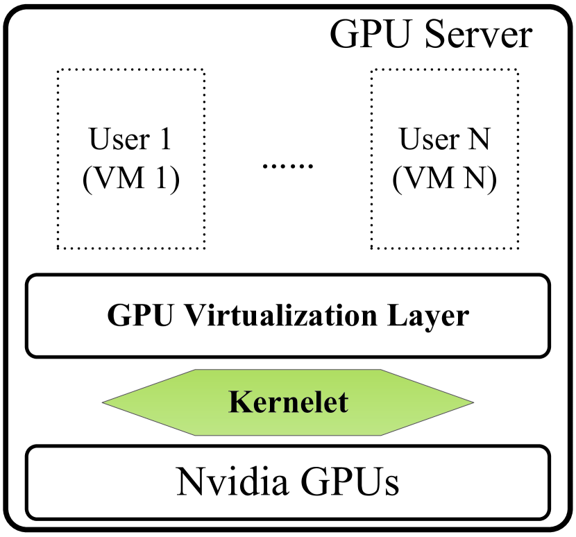
(a) GPU shared within one machine.

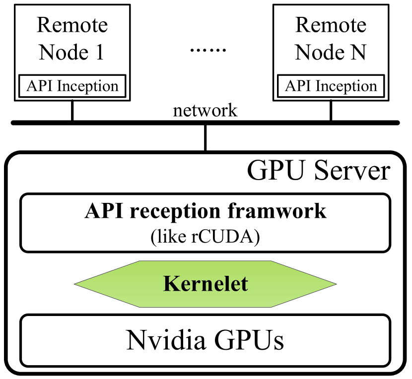
(b) GPU shared by remote clients.

Figure 1: Application scenarios of concurrent kernel executions on the GPUs.

Application scenario. We consider two typical application scenarios in the shared environments as shown in Figure 1. One is sharing the GPUs among multiple tenants in the virtualized environment (e.g., cloud). As illustrated in Figure 1(a), there is usually a GPU virtualization layer integrated with the hypervisor. Figure 1(b) shows the other scenario, in which GPU servers offer API reception softwares (like rCUDA [7, 45]) to support local/remote CUDA kernel launches. In both scenarios, the GPU faces multiple pending kernel launch requests. Kernelet can be applied to schedule those pending kernels.

Our study mainly considers the throughput issues of sharing a single GPU. Kernelet can be extended to multiple GPUs with a workload dispatcher to each individual GPU.

We have made the following assumptions on the kernels.

1. We target at the concurrent kernel executions on the shared GPU. The kernels are usually throughput oriented, with flexibility on the response time for scheduling. Still, we do not assume the a priori knowledge of the order of the kernel arrival.

2. Thread blocks in a kernel are independent with each other. This assumption is mostly true for the GPGPU kernels due to SPMD programming model. Most kernels in NVIDIA SDK and benchmarks like Parboil [13] do not have dependency among thread blocks in the same kernel. This assumption ensures that our slicing technique on a given kernel is safe. The data dependency among thread blocks can be identified with standard static or dynamic program analysis.

We formally define the terminology in Kernelet.

Kernel. A kernel $\mathcal{K}$ consists of $k$ thread blocks with IDs, 0, 1, 2, …, $(k-1)$.

Slice. A slice is a subset of the thread blocks of a launched kernel. Block IDs of a slice is continuous in the grid index space. The size of a slice $s$ is defined as the number of thread blocks contained in the slice.

Slicing plan. Given a kernel $\mathcal{K}$, a slicing plan $\mathcal{S}(\mathcal{K})$ is a scheme slicing $\mathcal{K}$ into a sequence of $n$ slices (${s}_{0}$, ${s}_{1}$, ${s}_{2}$, …, ${s}_{n-1}$). We denote the slicing plan to be $\mathcal{K}$=${s}_{0}$, ${s}_{1}$, ${s}_{2}$, …, ${s}_{n-1}$.

Co-schedule. Co-schedule ${cs}$ defines concurrent execution of $n$ ($n\geq 1$) slices, denoted as ${s}_{0}$, …, ${s}_{n-1}$. All the $n$ slices are active on the GPU.

Scheduling plan. Given a set of $n$ kernels $\mathcal{K}_{0}$, $\mathcal{K}_{1}$, …, $\mathcal{K}_{n}$, a scheduling plan $\mathcal{C}$ (${cs}_{0}$, ${cs}_{1}$, …, ${cs}_{n-1}$) determines a sequence of co-schedules in their order of execution. ${cs}_{i}$ is launched before ${cs}_{j}$ if $i<j$. All thread blocks of the $n$ kernels occur in one of the co-schedules once and only once. A scheduling plan embodies a slicing plan for each kernel.

We define the performance benefit of co-scheduling $n$ kernels to be the co-scheduling profit ($\mathit{CP}$) in Eq. (1). $IPC_{i}$ and $cIPC_{i}$ are IPC (Instruction Per Cycle) for sequential execution and concurrent execution of kernel $i$ respectively. Our definition is similar to those in the previous studies on CPU multi-threaded co-scheduling [20, 39].

$$\mathit{CP}=1-\frac{1}{\sum\limits_{i=1}^{n}\frac{cIPC_{i}}{IPC_{i}}}$$ (1)

Problem definition. Given a set of kernels for execution, the problem is to determine the optimal scheduling plan (and slicing) so that the total execution time for those kernels is minimized. That corresponds to the maximized throughput. Given a set of $n$ kernels $\mathcal{K}_{0}$, $\mathcal{K}_{1}$, …, $\mathcal{K}_{n-1}$, we aim at finding the optimal scheduling plan $\mathcal{C}$ for a minimized total execution time of $\mathcal{C}($$\mathcal{S}_{0}(\mathcal{K}_{0})$, $\mathcal{S}_{1}(\mathcal{K}_{1})$, …, $\mathcal{S}_{n-1}(\mathcal{K}_{n-1})$), or maximized co-scheduling profit. Note, in the shared GPU environment, the arrival of new kernels trigger the recalculation of the optimization on the kernel residuals and new kernels.

3 System Overview

In this section, we present the rationales on the Kernelet design, followed by an overview of the Kernelet runtime.

3.1 Design Rationale

Since kernels are submitted in an ad-hoc manner in our application scenarios, the scheduling decision has to be made at real time. The optimization process should take the newly arrived kernels into consideration. Moreover, our runtime system of slicing and scheduling should be designed with light overhead. That is, the overhead of slicing and scheduling should be small compared with their performance gain.

Unfortunately, finding the optimal slicing plans and scheduling plan is a challenging task. The solution space for such candidate plans is large. For slicing a kernel, we have the factors including the number of slices as well as the slice size. For scheduling a set of slices, we can generate different scheduling plan with co-scheduling slices from different kernels. All those factors are added up into a large solution space. Considering newly arrival kernels makes the huge scheduling space even larger.

Due to the real-time decision making and light-weight requirements, it is impossible to search the entire space to get a globally optimal solution. The classic Monte Carlo simulation methods are not feasible because they usually exceed our budget on the runtime overhead and violate real-time decision making requirement. There must be a more elegant compromise between the optimality and runtime efficiency. Our solution to the scheduling problem is detailed in Section 4.2.

Given the complexity of dynamic slicing and scheduling in concurrent kernel executions, we make the following considerations.

First, the scheduling considers two kernels only. Previous studies [20] on the CPU have shown that when there are more than two co-running jobs, finding the optimal scheduling plan becomes an NP-complete problem even ignoring the job length differences and rescheduling. Following previous studies [20, 34], we make our scheduling decision co-scheduling two kernels only.

Second, once we choose two kernels to schedule, their slice sizes keep unchanged until either kernel finishes. The suitable slice size is determined according to our performance model 4.4.

3.2 System Overview

We develop Kernelet as a runtime system to generate the slicing plan and scheduling plans for the optimized throughput.

Figure 2 shows an overview of Kernelet. Kernels are submitted and are temporarily buffered in a kernel queue for further scheduling. Usually, a kernel is submitted in the form of binary (SASS) or PTX code. Submitted kernels are first preprocessed by kernel slicer to determine the smallest slice size for a given overhead limit. If the kernel has been submitted before, we simply use the smallest slice size in the previous execution. Kernelet’s scheduler determines the scheduling plan based on the results of performance model, which estimates the performance of slices from two different kernels in a probabilistic manner. Once the scheduling plan is obtained, slices are dispatched for execution on the GPU. We will describe the detailed design and implementation of each component in the next section.

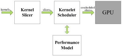
Figure 2: Design overview of Kernelet.

4 Kernelet Methodology

In this section, we first describe our kernel slicing mechanism. Next, we present our greedy scheduling algorithm, followed by our pruning techniques on the co-schedule space and the description of the performance model.

4.1 Kernel Slicing

The purpose of kernel slicing is to divide a kernel into multiple slices so that the finer granularity of each slice as a kernel in the scheduling can create more opportunities for time sharing. Moreover, we need to determine the suitable slice size for minimizing the slicing overhead (i.e., between the total execution time of all slices and the kernel execution time) . Particularly, we experimentally determine the suitable slice size to be the minimum slice so that the overhead is not greater than $p\%$ of the kernel execution time. In this study, $p\%$ is set to be 2% by default. We focus on the implementation of slicing on PTX or SASS code. Note that, warps within the same thread block usually have data dependency with each other, e.g., with the usage of shared memory. That is why we choose thread blocks as the units for slicing, instead of warps.

Figure 3 illustrates the sliced execution of $\mathit{MatrixAdd}$ with pseudo code. In the example, $\mathit{MatrixAdd}$ is a GPU kernel to add two $256\times 256$ matrices and each thread adds one element pair from the input matrices. Based on the matrix size, $\mathit{MatrixAdd}$ is configured to launch with $16\times 16$ thread blocks in total and each block has $16\times 16$ threads. Figures 3(a) and 3(b) illustrate the definition and launch of the original kernel, respectively. In comparison, the sliced version of the kernel launches a slice with 8 thread blocks each time. The built-in thread block indices (denoted as $\mathit{blockID\_X}$ and $\mathit{blockID\_Y}$) of the sliced kernel are in a smaller index space ($\{(x,0)|0\leq x<8\}$) compared with the original index space ($\{(x,y)|0\leq x<16\ and\ 0\leq y<16\}$). To make the slices execute as individual kernels, we apply a procedure called index rectification. As shown in Figure 3(c), we add an offset value to the thread block indices and obtain the rectified index values. The rectified indices are used to replace all subsequent accesses to the built-in indices. On the CPU side, we launch the slices in a loop and adjust the offset values for each slice launch (Figure 3(d)).

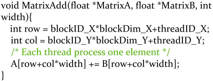
(a) Each thread access the corresponding matrix element using block and thread indices.

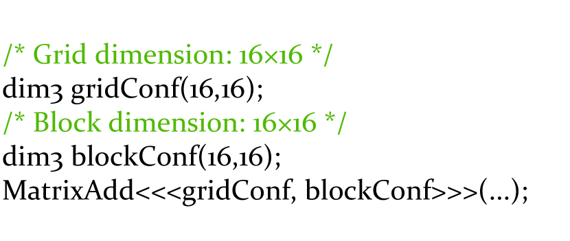
(b) Launch the same number threads as the number of matrix elements.

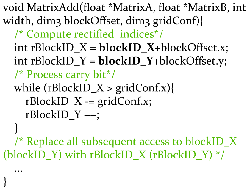
(c) Sliced kernel with rectified thread block indices.

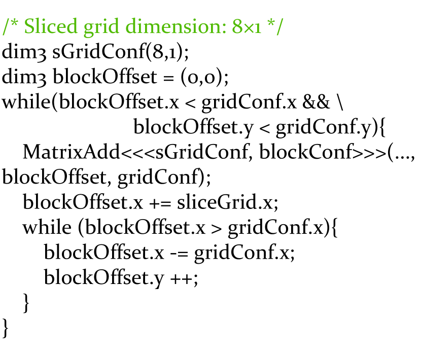
(d) Launch all slices of a kernel in a loop.

Figure 3: An example of kernel slicing.

Kernelet automatically implements slice rectification without any user intervention. With PTX or SASS code as input, Kernelet does not require source code. Kernelet interprets and modifies the PTX/SASS code at runtime. The resulting PTX code is compiled to GPU executables by the GPU driver, and the SASS code is assembled using the open source Fermi assembler Asfermi [1]. Kernelet stores the rectified block index in registers, and replaces all references to those built-in variables with the new registers. Since this process may use more registers. Kernelet tries to minimize the register usage by adopting the classic register minimization techniques [33, 5], e.g., variable liveness analysis. With register optimizations, register usage by slicing keeps unchanged in most of our test cases in experiments. Note, kernel slicing only requires a single scan on the input code and the runtime overhead is negligible.

4.2 Scheduling

According to our design rationales, our scheduling decision is made on the basis of two kernels, to avoid the complexity of scheduling three or more kernels as a whole; the slice sizes of the two kernels are tuned for GPU utilization so that their execution times in the concurrent kernel execution are close. Thus, we develop a greedy scheduling algorithm, as shown in Algorithm 1. The scheduling algorithm considers new arrival kernels in Lines 2–3 in the main algorithm. The main procedure calls the procedure FindCoSchedule to obtain the optimal co-schedule in Line 5. The co-schedule is represented in four parameters $<$ $\mathcal{K}_{1}$, $\mathcal{K}_{2}$, $\mathit{size}_{1}$, $\mathit{size}_{2}$ $>$, where $\mathcal{K}_{1}$ and $\mathcal{K}_{2}$ denotes the two selected kernels; $\mathit{size}_{1}$ and $\mathit{size}_{2}$ represents the slice sizes accordingly. We use the same co-schedule if the kernels pending for execution do not change, or both kernels still have thread blocks.

Algorithm 1 Scheduling algorithm of Kernelet

1:  Denote $\mathcal{R}$ to be the set of kernels pending for executions;

2:  if A new kernel $\mathcal{K}$ comes then

3:     Add $\mathcal{K}$ into $\mathcal{R}$;

4:  while $\mathcal{R}$!=null do

5:     $<$ $\mathcal{K}_{1}$, $\mathcal{K}_{2}$, $\mathit{size}_{1}$, $\mathit{size}_{2}$ $>$=FindCoSchedule($\mathcal{R}$);

6:     Denote the co-schedule to be $c$;

7:     Execute $c$ on the GPU;

8:     while $\mathcal{R}$ does not change, or $\mathcal{K}_{1}$ and $\mathcal{K}_{2}$ both still have thread blocks do

9:        Generate co-schedule according to $c$ and execute it on the GPU;

Proc. FindCoSchedule($\mathcal{R}$)
Function: generate the optimal co-schedule from $\mathcal{R}$.

1:  Generate the candidate space for co-schedules $\mathcal{C}$;

2:  Perform pruning on $\mathcal{C}$ according to the computation and memory characteristics of input kernels;

3:  Apply the performance model (Section 4.4) to compute $\mathit{CP}$ for all the co-schedule in $\mathcal{C}$;

4:  Obtain the optimal co-schedule with the maximized $\mathit{CP}$;

5:  Return the result co-schedule;

In Procedure FindCoSchedule, we first consider the entire candidate space consisting of co-schedules on pair-wise kernel combinations. Because the space may consider of $\frac{N(N-1)}{2}$ co-schedules ($N$ is the number of kernels for consideration), it is desirable to reduce the search space. Therefore, we perform pruning according to the computation and memory characteristics of input kernels. We present the details of pruning mechanisms in Section 4.3. After pruning, we apply the performance model (Section 4.4) to estimate the $\mathit{CP}$ for all co-schedules, and pick the one with the maximized $\mathit{CP}$ for executing on the GPU.

4.3 Co-scheduling Space Pruning

Given a set of co-schedules as input, we aim at developing pruning techniques to remove the co-schedules that are not “promising” to deliver performance gain. So that the overhead of running the performance model is avoided. The basic idea to identify the key performance factor of a single kernel that affects the throughput of concurrent kernel executions on the GPU.

There are many factors affecting the GPU performance. According to the CUDA profiler, there are around 100 profiler counters and statistics for the performance tuning. For an effective scheduling algorithm, there is no way of considering all these factors. Following a previous work [24], we use the regression model to explore the correlation between the above mentioned factors and $\mathit{CP}$. The input values are obtained from single kernel executions. Through detailed performance studies, we find that instruction throughput and memory bandwidth utilization are the most correlated performance factors with co-scheduling friendliness. We define PUR (Pipeline Utilization Ratio) and MUR (Memory-bandwidth Utilization Ratio) to characterize user submitted kernels. High PUR means the instruction pipeline is highly utilized and there is little room for performance improvement. High MUR means a large number of memory requests are being processed and memory latency is high. PUR and MUR is calculated as follows,

$$PUR=\frac{Instruction\_Executed}{Time\times Frequency\times Peak\_IPC}$$

$$MUR=\frac{Dram\_Reads+Dram\_Writes}{Time\times Frequency\times Peak\_MPC}$$

$Peak\_IPC$ and $Peak\_MPC$ represent peak number of instructions and memory requests per cycle respectively. $Instruction\_Executed$ is the total number of instructions executed. $Dram\_Reads$ and $Dram\_Writes$ are the numbers of read and write requests to DRAM respectively.

We build a set of testing kernels to demonstrate the correlation between PUR/MUR and $\mathit{CP}$. A testing kernel is a mixture of memory and computation instructions. We tune the respective instruction ratios to obtain kernels with different memory and computational characteristics. The single kernel execution PURs and MURs of the testing kernels are in the range of $[0.26,0.83]$ and $[0.07,0.84]$ respectively. Figure 4 shows the strong correlation between MUR/PUR and $\mathit{CP}$. The observation conforms to our expectation. First, if one kernel has high PUR while the other kernel has low PUR, the former kernel is able to utilize the idle cycles exposed by the latter kernel when co-scheduled. Second, co-scheduling kernels with complementary memory requirements (one kernel has low MUR and the other kernel has high MUR) will alleviate memory contention and reduce idle cycles exposed by long latency memory operations.

In summary, our pruning rule is to remove the co-schedules where the two kernels have close PUR or MUR values. We set two threshold values $\alpha_{p}$ and $\alpha_{m}$ for PUR and MUR, respectively. That means, we prune the co-schedule if the two kernels have PUR difference lower than $\alpha_{p}$, or have MUR difference lower than $\alpha_{m}$. Note, if all the co-schedules are pruned, we need to increase $\alpha_{p}$ or $\alpha_{m}$. We experimentally evaluate the impact of those two threshold values in Section 5.

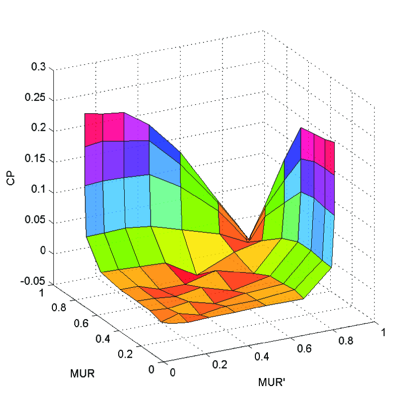
(a) MUR and $\mathit{CP}$

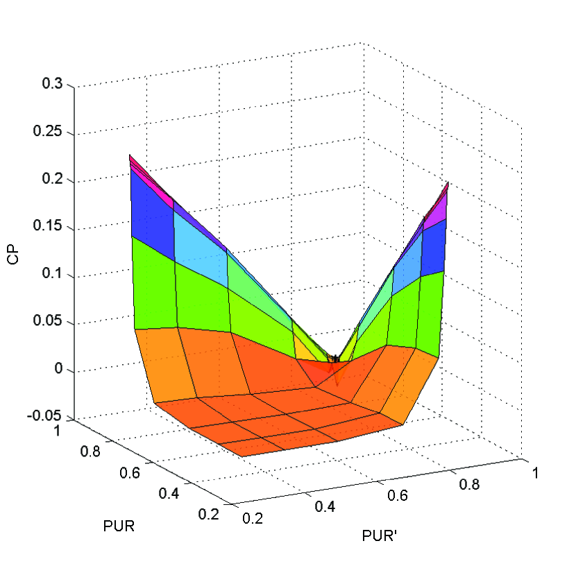
(b) PUR and $\mathit{CP}$

Figure 4: Correlation between MUR/PUR and $\mathit{CP}$

4.4 Performance Model

We need a performance model for two purposes: firstly, to select the two kernels for co-schedule; secondly, to determine the number of thread blocks for each kernel in the co-schedule (i.e., the slice size). Previous performance models on the GPU [19, 38, 44] assume a single kernel on the GPU, and are not applicable to concurrent kernel executions. They generally assume that the thread blocks execute the same instruction in a round-robin manner on an SM. However, this is no longer true on concurrent kernel executions. The thread blocks from different kernels have interleaving executions, which cause non-determinism on the instruction execution flow. It is not feasible to statically predict the interleaving warp executions for multi-kernel executions. To capture the non-determinism, we develop a probabilistic performance model to estimate the performance of co-schedule. Our cost model has very low runtime overhead, because it uses a series of simple parameters as input and leverages the Markov chain theory to get the performance of concurrent kernel executions.

Table I summarizes the notations used for our performance model.

TABLE I: Parameters and notations in the performance model

Para.	Description
$W$	Maximum number of active warps
$Round$	A warp scheduling cycle that all ready warps are served by the warp scheduler
$R_{m}$	Memory instruction ratio
$P_{r\rightarrow r}$	Probability that a ready warp remains ready
$P_{r\rightarrow i}$	Probability that a ready warp transits to idle
$P_{i\rightarrow r}$	Probability that an idle warp transits to ready
$P_{i\rightarrow i}$	Probability that an idle warp remains in idle
$N_{r\rightarrow r}$	Number of ready warps that remain ready
$N_{r\rightarrow i}$	Number of ready warps that transit to idle
$N_{i\rightarrow r}$	Number of idle warps that transit to ready
$N_{i\rightarrow i}$	Number of idle warps that remain idle
$L$	Average memory latency (cycle)
$B$	GPU global memory bandwidth (requests/cycle)
$S_{i}$	$S_{i}$ corresponds the state where $i$ warps are idle on the SM ($i=0,1,\ldots,W$)
$P_{ij}$	$P$ is the Markov chain transit matrix. Entry $P_{ij}$ of $P$ represents the probability of transiting from state $S_{i}$ to state $S_{j}$.

Since the GPU adopts SPMD model, we use the performance estimation of one SM to represent the aggregate performance of all SMs on the GPU. We model the process of kernel instruction issuing as a stochastic process and devise a set of states for an SM during execution. By modeling the SM state, we first develop our Markov chain based models for single-kernel executions (homogeneous workloads), and then extend it to concurrent kernel executions (heterogeneous workloads).

For presentation clarity, we begin with our description on the model with the following assumptions, and relax those assumptions at the end of this section. First, we assume that all the memory requests are coalesced. This is the best case for memory performance. We will relax this assumption by considering both coalesced and uncoalesced memory accesses. Second, we assume that the GPU has a single warp scheduler. We will extend it to the GPU with multiple warp schedulers.

Homogeneous Workloads. We first investigate the performance of a single kernel executed on the GPU and each SM accommodates $W$ active warps at most.

A warp can be in two states: idle or ready. An idle warp is stalled by memory accesses, and a ready warp has one instruction ready for execution. Its transition is illustrated in Figure 5. When a warp is currently in the ready state, we have two cases for state transitions by definition:

• remaining in the ready state with the probability of $P_{r\rightarrow r}=1-R_{m}$.

• transiting to the idle state with the probability of $P_{r\rightarrow i}=R_{m}$.

When a warp is currently in the idle state, we also have two cases for state transitions:

• transiting to the ready state with the probability of $P_{i\rightarrow r}=\frac{1}{\frac{L}{W-I}}=\frac{W-I}{L}$, where $I$ is the number of idle warps on the SM.

• remaining in the idle state with the probability of $P_{i\rightarrow i}=1-P_{i\rightarrow r}$.

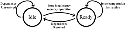
Figure 5: Warp state transition diagram.

We specifically define the time step and state transition of the Markov chain model to capture the GPU architectural features. GPU adopts a round-robin style scheduling [19]. In each round, the warp scheduler polls each warp to issue its ready instructions so all ready warps can make progress. We model the SM state with the number of idle warps. We denote $S_{i}$ to be the SM state where $i$ warps are idle on the SM ($i=0,1,\ldots,W$). Thus, we consider the state change of the SM in one round and use round as time step in our Markov chain model. In each round, every ready warp has an equal chance to issue instructions. In contrast, models for the CPU assume that the CPU will keep executing one thread until this thread is suspended.

We use $\mathit{IPC}$ to represent the throughput of the SM. Thus, the number of idle warps on the SM is a key parameter for $\mathit{IPC}$. Thus, we define the state of SM as the number of idle warps on the SM (i.e., the state is $S_{i}$ when the number of idle warps is $i$). More outstanding memory requests usually lead to higher latency because of memory contention [3]. We adopt a linear memory model to account for the memory contention effects. We calculate $L$ as $L=L_{0}+\frac{B}{a_{0}\cdot S_{i}}+b_{0}$, where $a_{0}$ and $b_{0}$ are the constant parameters in the linear model. We obtain $L_{0}$ and $B$ according to hardware specifications.

For homogeneous workload, the probabilities of state transitions are the same for all ready warps in a round. We assume when SM transits from $S_{i}$ to $S_{j}$, $N_{i\rightarrow r}$ idle warps transit to the ready state and $N_{r\rightarrow i}$ ready warps transit to idle state. The following conditions hold by definition.

$$\begin{cases}0\leq N_{i\rightarrow r}\leq S_{i}\\ 0\leq N_{r\rightarrow i}\leq W-S_{i}\\ N_{r\rightarrow i}-N_{i\rightarrow r}=S_{j}-S_{i}\end{cases}$$ (2)

With those constraints, there are multiple possible transitions to transit from $S_{i}$ to $S_{j}$. Since the possible transitions are mutually exclusive events, the probability of each state transition $P_{ij}$ is calculated as the sum of the probabilities of all possible transitions. With all entries of the transition matrix $P$ obtained, we can calculate the steady-state vector of the Markov chain. This is done by finding the eigenvector $\pi$ corresponding to the eigenvalue one for matrix $P$ [31].

$$\pi=(\gamma_{0},\gamma_{1},...,\gamma_{W})$$ (3)

In Equation 3, $\gamma_{i}$ is the probabilities that the SM stays in state $S_{i}$ in each round, i.e., the probability there are $i$ idle warps in one round. The duration of the time step is $(W-i)$ cycles since each of the $(W-i)$ ready warps issue one instruction within the round. In the case $i=W$, the round duration is one, indicating no warp is ready and the SM experiences an idle cycle. Hence, the estimated $\mathit{IPC}$ is the ratio of non-idle cycles given in equation 4, where $\sum_{i=0}^{W-1}\gamma_{i}(W-i)$ is the total non-idle cycles and $\gamma_{W}$ is the total idle cycles.

$$IPC_{\mathcal{K}}=\frac{\sum_{i=0}^{W-1}\gamma_{i}(W-i)}{\sum_{i=0}^{W-1}\gamma_{i}(W-i)+\gamma_{W}}$$ (4)

Heterogeneous Workloads. When there are multiple kernels running concurrently, the model needs to keep track of the state of each workload. Although we only consider two concurrent kernels ($\mathcal{K}_{1}$ and $\mathcal{K}_{2}$) in scheduling, our model can be used to handle more than two kernels.

Suppose there are two kernels $\mathcal{K}_{1}$ and $\mathcal{K}_{2}$, and $\mathcal{K}_{1}$ has $w_{1}$ active warps and $\mathcal{K}_{2}$ has $w_{2}$ active warps $(w_{1}+w_{2}=W)$. The number of possible states of the SM will be $(w_{1}+1)\times(w_{2}+1)$. The state space is represented as a pair $(p,q)$ with $0\leq p\leq w_{1}$ and $0\leq q\leq w_{2}$, where $p$ and $q$ are the numbers of idle warps of $\mathcal{K}_{1}$ and $\mathcal{K}_{2}$ respectively. We can calculate the probability of transiting from state $(p_{i},q_{i^{\prime}})$ to state $(p_{j},q_{j^{\prime}})$ by first considering individual workload state transition probability using the single kernel model, and then calculating the SM state transition probability. The state transitions of different kernels are independent with each other, because the kernels are independent. Then the SM state transition probability is the product of the individual transition probabilities.

With Markov chain approach, we obtain the steady state vector $\pi=\{\gamma_{(0,0)},\gamma_{(0,1)},...,\gamma_{(w_{1},w_{2})}\}$. Next, we can obtain the $\mathit{IPC}$ of each workload using the same method as the model in single-kernel executions, except the parameters are defined and calculated in the context of two kernels. For example, the round duration is equal to the total number of ready warps of both kernels. Individual IPCs of $\mathcal{K}_{1}$ and $\mathcal{K}_{2}$ is calculated as the ratio of non-idle cycles for each workload, as shown in Eq. (5) and (6), respectively. The concurrent IPC is the sum of individual IPCs Eq. (7). Then $\mathit{CP}$ can be obtained using Eq. (1).

$$IPC_{\mathcal{K}_{1}}=\frac{\sum_{i=0}^{w_{1}-1}\sum_{i^{\prime}=0}^{w_{2}}\gamma_{(i,i^{\prime})}\times(w_{1}-i)}{\sum_{i=0}^{w_{1}}\sum_{j=0}^{w_{2}}\gamma_{(i,j)}\times R_{(i,j)}}$$ (5)

$$IPC_{\mathcal{K}_{2}}=\frac{\sum_{i=0}^{w_{1}}\sum_{i^{\prime}=0}^{w_{2}-1}\gamma_{(i,i^{\prime})}\times(w_{2}-i^{\prime})}{\sum_{i=0}^{w_{1}}\sum_{i^{\prime}=0}^{w_{2}}\gamma_{(i,i^{\prime})}\times R_{(i,i^{\prime})}}$$ (6)

$$C=IPC_{\mathcal{K}_{1}}+IPC_{\mathcal{K}_{2}}$$ (7)

With the estimated IPC and $\mathit{CP}$, we now discuss how to estimate the optimal slice size ratio for two kernels. We define the slice ratio which minimizes the execution time difference of co-scheduled slices as the balanced slice ratio. By minimizing the execution time difference, the kernel-level parallelism is maximized. The execution time difference is calculated as $\Delta T$ in Eq. (8).

$$\begin{array}[]{lcl}\Delta T=|\frac{1}{\mathit{IPC_{\mathcal{K}_{1}}}}\times I_{\mathcal{K}_{1}}\times P_{\mathcal{K}_{1}}-\frac{1}{IPC_{\mathcal{K}_{2}}}\times I_{\mathcal{K}_{2}}\times P_{\mathcal{K}_{2}}|\\ \end{array}$$ (8)

$I_{\mathcal{K}_{i}}$ and $P_{\mathcal{K}_{i}}$ represent the number of instruction per block and the slice size of kernel $\mathcal{K}_{i}$ ($i=1,2$) in number of thread blocks. Since $P_{\mathcal{K}_{i}}$ is less than the maximal number of active thread blocks, only a limited number of slice ratios need to be evaluated to get the balanced ratio.

Uncoalesced Access. So far, we assume that all memory accesses are coalesced and each memory instruction results in the same number of memory requests. However, due to the different address patterns, memory instructions may result in a different amount of memory requests. On Fermi GPUs, one memory instruction can generate 1 to 32 memory requests. Here we consider the two most common access patterns: fully coalesced access, and fully uncoalesced access. We extend our model to handle both coalesced and uncoalesced accesses by defining three states for a warp: ready, stalled on coalesced access (uncoalesced idle), and stalled on uncoalesced access (coalesced idle). The memory operation latency depends on the memory access type. Since uncoalesced access generates more memory traffic, its latency is higher than coalesced access. We also use the linear model to estimate the latency. By identifying the ratio of coalesced and uncoalesced memory instructions, we can easily extend the two-state model to handle three states and their state transitions. The Markov chain performance model can be developed in a similar way. Distinguishing between coalesced and uncoalesced accesses increases the accuracy of our model.

Adaptation to GPUs with multiple warp schedulers. Our model assumes there is only one warp scheduler. New-generation GPUs can support more than one warp schedulers. The latest Kepler GPU features four warp schedulers per SMX (SMX is the Kepler terminology for SM) [28]. We extend our model to handle this case by deriving a single pipeline virtual SM based on the parameters of the SMX. The virtual SM has one warp scheduler, and its parameters such as active thread blocks and memory bandwidth are obtained by dividing the corresponding parameters of the SMX by the number of warp schedulers. This virtual SM can still capture the memory and computation features of a kernel running on the SMX. Experimental results in Section 5 show that performance modeling on the virtual SM provides a good estimation on the Kepler architectures.

There are two more issues that are worthwhile to discuss.

The first issue is on the efficiency of executing our model at runtime. We have developed mechanisms to make our model more efficient without significantly sacrificing the model accuracy. The $O(N^{3})$ complexity of calculating the steady state in Markov chain makes it hard to meet the online requirement ($N$ is the dimension of the transition matrix). To reduce the computational complexity, we consider the thread block as a scheduling unit, instead of considering individual warps. In this way, the computational complexity is significantly reduced, and time cost of our model is negligible to the GPU kernel execution time.

The second issue is on getting the input for the model. Our current approach is based on hardware profiling of a small number of thread blocks from a single kernel. Thus, the pre-execution is only a very small part of the kernel execution. From profiling, we can obtain the number of memory instructions issued and the total number of instructions executed, and calculate $\mathit{Rm}$ as their ratio.

In summary, our probabilistic model has captured the inherent non-determinism in concurrent kernel executions. First, it simply requires only a small set of profiling inputs on the memory and computation characteristics of individual kernels. Second, with careful probabilistic modeling, we develop a performance model that is sufficiently accurate to guide our scheduling decision. The effectiveness of our model will be evaluated in the experiments (Section 5).

5 Evaluation

In this section, we present the experimental results on evaluating Kernelet on latest GPU architectures.

5.1 Experimental Setup

We have conducted experiments on a workstation equipped with one NVIDIA Tesla C2050 GPU, one NVIDIA GTX680 GPU, two Intel Xeon E5645 CPUs and 24GB RAM. Table II shows some architectural features of C2050 and GTX680. We note that C2050 and GTX680 are based on Fermi and Kepler architectures, respectively. One C2050 SM has two warp schedulers, and each can serve half a warp per cycle (with a theoretical $\mathit{IPC}$ of one). In contrast, one GTX680 SMX features four warp schedulers and each warp scheduler can serve one warp per cycle (with a theoretical $\mathit{IPC}$ of eight considering its dual-issue capability). Our implementation is based on GCC 4.6.2 and NVIDIA CUDA toolkit 4.2.

TABLE II: GPU configurations.

	C2050	GTX680
Architecture	Fermi GF110	Kepler GK104
Number of SMs	14	8
Number of cores per SM	32	192
Core frequency (MHz)	1147	706
Global memory size (MB)	3072	2048
Global memory bandwidth (GB/s)	144	192

Workloads. We choose eight benchmark applications with different memory and computation intensivenesses. Sources of the benchmarks include the CUDA SDK, the Parboil Benchmark [13], the CUSP library [4] and our home grown applications. Table III describes the details of each application, including input settings and thread configurations of the most time-consuming kernel on C2050.

Table IV shows the memory and computation characteristics of the most time-consuming kernel of each application on both C2050 and GTX680. We observed that the PUR/MUR values are stable as we vary the input sizes (as long as the input size is sufficiently large to keep the GPU occupancy high).

TABLE III: Specification of benchmark applications and thread configuration (#threads per thread block $\times$ #thread blocks).

Name	Description	Input settings	Thread configuration on C2050
Pointer Chasing (PC)	Traversing an array randomly	Index values for 40 million accesses	256 $\times$ 16384
Sum of Absolute Differences (SAD)	An operation used in MPEG encoding	Image with $1920\times 1072$ pixels	32 $\times$ 8048
Sparse Matrix Vector Multiplication (SPMV)	Multiplying a sparse matrix with a dense vector.	A 131072$\times$81200 matrix with 16 non-zero elements per row on average	256 $\times$ 16384
Stencil (ST)	Stencil operation on a regular 3-D grid	3D grid with 134217728 points	128 $\times$ 16384
Matrix Multiplication (MM)	Multiplying two dense matrices	One $8192\times 2048$ matrix, the other $2048\times 2048$	256 $\times$ 16384
Magnetic Resonance Imaging - Q (MRIQ)	A matrix operation in magnetic resonance imaging	2097152 elements	256 $\times$ 8192
Black Scholes (BS)	Black-Scholes Option Pricing	40 million	128 $\times$ 16384
Tiny Encryption Algorithm (TEA)	A thread block cipher	20971520 elements	128 $\times$ 16384

TABLE IV: Memory and computational characteristics of benchmark applications.

Benchmarks	C2050			GTX680
	PUR	MUR	Occupancy	PUR	MUR	Occupancy
PC	0.0096	0.1404	100%	0.0072	0.1746	100%
SAD	0.1498	0.1120	16.7%	0.1062	0.1351	25%
SPMV	0.3464	0.003	100%	0.3027	0.0043	100%
ST	0.3629	0.1156	66.7%	0.2016	0.1179	100%
MM	0.5804	0.0161	67.7%	0.5321	0.0569	100%
MRIQ	0.8539	0.0002	83.3%	1.6784	0.0007	100%
BS	0.8642	0.0604	67.7%	1.2007	0.1323	100%
TEA	0.9978	0.0196	67.7%	1.1417	0.0353	100%

To assess the impact of kernel scheduling under different mixes of kernels, we create four groups of kernels namely CI, MI, MIX and ALL (as shown in Table V). CI represents the computation-intensive workloads including kernels with high PUR, whereas MI represents workloads with intensive memory accesses. MIX and ALL include a mix of CI and MI kernels. ALL has more kernels than MIX. In each workload, we assume the application arrival conforms to Poisson distribution. The parameter $\lambda$ in the Poisson distribution affects the weight of the application in the workload. For simplicity, we assume that all application has the same $\lambda$. We also assume $\lambda$ is sufficiently large so that at least two kernels are pending for execution at any time for a high utilization of the GPU.

TABLE V: Workload configurations.

Workload	Applications
CI	BS, MM, TEA, MRIQ
MI	PC, SPMV, ST, SAD
MIX	PC, BS, TEA, SAD
ALL	PC, SPMV, ST, BS, MM, TE, MRIQ, SAD

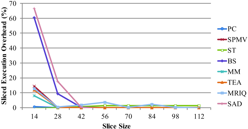
(a) C2050

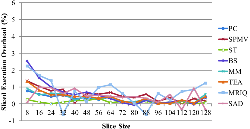
(b) GTX680

Figure 6: Sliced execution overhead with varying slice size on both C2050 and GTX680.

Comparisons. To evaluate the effectiveness of kernel scheduling in Kernelet, we have implemented the following scheduling techniques:

• Kernel Consolidation (BASE): the kernel consolidation approach of concurrent kernel execution [34].

• Oracle (OPT): OPT uses the same scheduling algorithm as Kernelet, except that it pre-executes all possible slice ratios for all combinations to obtain the $\mathit{CP}$ and then determines the best slice ratio and kernel combination. In another word, OPT is an offline algorithm and provides the optimal throughput for the greedy scheduling algorithm.

• Monte Carlo-based co-schedule (MC): we develop a Monte Carlo approach to generate the distribution of performance of different co-schedule methods in the solution space. In each Monte Carlo simulation, we randomly pick the kernel pairs and slice ratios for co-scheduling. Through many Monte Carlo simulations, we can quantitatively understand how different co-schedules affect the performance. We denote the result of MC to be MC($s$), where $s$ is the number of Monte Carlo simulations.

5.2 Results on Kernel Slicing

We first evaluate the overhead of sliced execution, which is defined as $\frac{T_{s}}{T_{\mathit{ns}}}-1$, where $T_{s}$ and $T_{\mathit{ns}}$ are the sliced and unsliced execution time, respectively.

Figure 6 shows the overhead for executing individual kernels with varying slice sizes on C2050 and GTX680. Slice sizes are set to multiples of the number of SMs on the GPU and ranges from $|\mathit{SM}|$ to the maximum number under the occupancy limit. Overall, as the slice size increases, the slicing overhead decreases. However, we observe quite different performance behaviors on C2050 and GTX680, due to their architectural differences. On C2050, when the size is small, the slicing overhead is very high (up to 66.7% for SAD). When the slice is larger than or equal to 42 (three thread blocks per SM), the overhead is ignorable for most kernels. Sliced execution overhead on GTX680 is much smaller than on C2050. Almost all slice sizes lead to overhead less than 2% on GTX680. Regardless of the architectural differences, the ignorable overhead of kernel slicing allows us to exploit kernel slicing for co-scheduling slices from different kernels with little additional cost.

5.3 Results on Model Prediction

We evaluate the accuracy of our performance model in different aspects, including the estimation of $\mathit{IPC}$s for single kernels and concurrent kernel executions, and $\mathit{CP}$ prediction for concurrent kernel executions.

Single Kernel Performance Prediction. Figure 7 compares the measured and estimated $\mathit{IPC}$ values for the eight benchmark applications on C2050 and GTX680. We also show the two lines ( $y=x\pm 0.2$ for C2050 and $y=x\pm 1.6$ for GTX680) to highlight the scope where difference between measurement and estimation is within $\pm$ 20% of the peak IPC. Note, the theoretical IPCs for C2050 and GTX680 are one and eight respectively. If the result falls in this scope, we consider the estimation well captures the trend of the measurement. We can see that, most results are within the scope. We further define the absolute error to be $\left|e-e^{\prime}\right|$, where $e$ and $e^{\prime}$ are the measured and estimated $\mathit{IPC}$ values, respectively. The average absolute error for the eight benchmark applications is 0.08 and 0.21 on C2050 and GTX680, respectively. Our probabilistic model has achieved a reasonable accuracy in estimating the performance of single-kernel executions on the GPU.

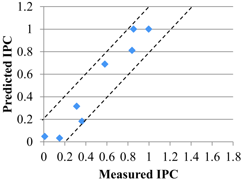
(a) C2050

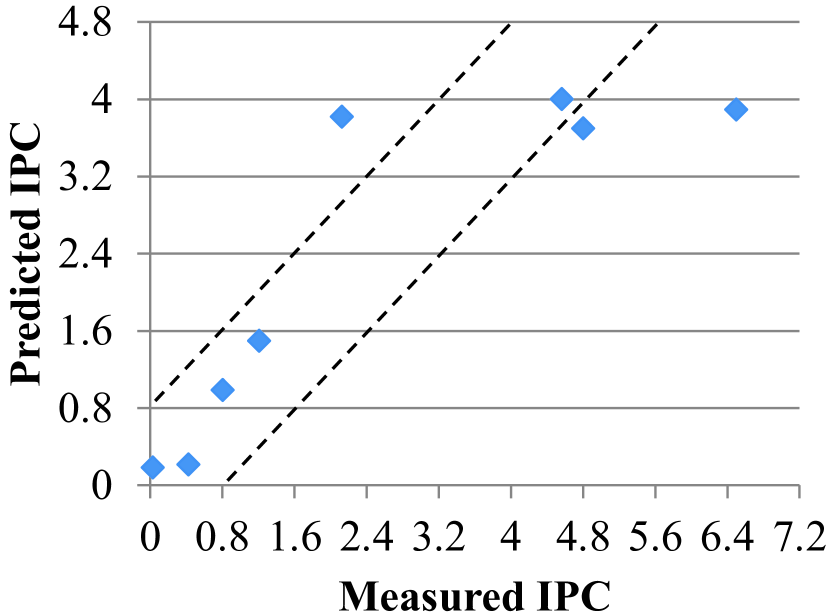
(b) GTX680

Figure 7: Comparison between predicted and measured single kernel execution IPCs on two GPUs.

Concurrent Kernel Performance Prediction. For the eight benchmark applications, we run every possible combination of kernel pairs and measure the $\mathit{IPC}$ for each combination. Figure 8 compares the measured and predicted $\mathit{IPCs}$ with the suitable slice ratio given by our model. We have also studied other slicing ratios. Figure 9 compares the measured and predicted $\mathit{IPCs}$ with fixed $\mathit{ratio}=1:1$. We observed similar results on other fixed ratios. Regardless of different kernel combinations and slicing ratios, our model is able to well capture the trend of concurrent executions for both dynamic and static slice ratios.

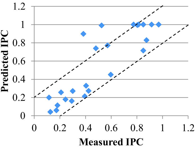
(a) C2050

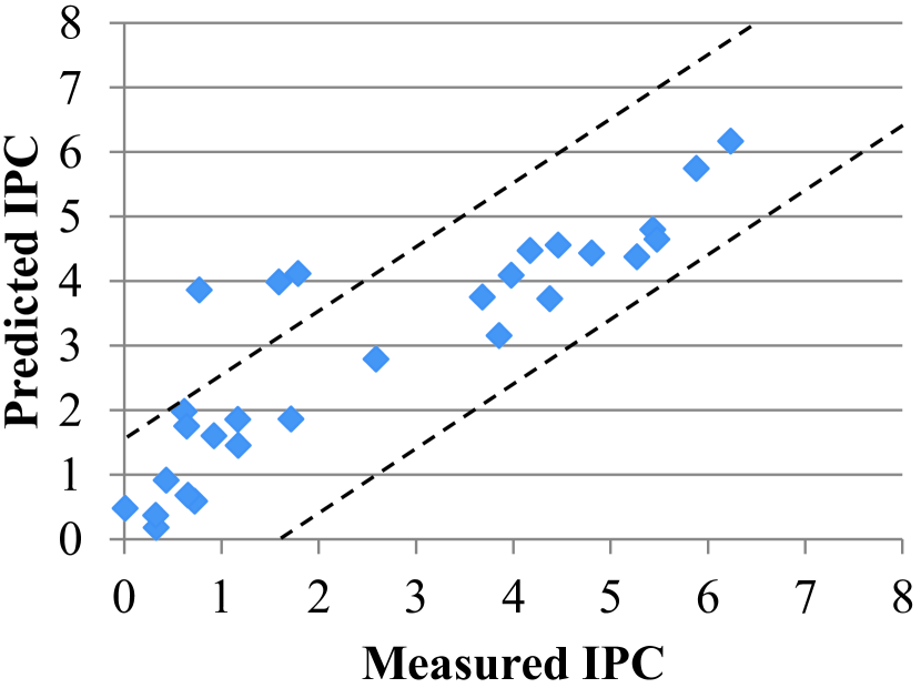
(b) GTX680

Figure 8: Comparison between predicted and measured concurrent kernel execution IPCs on two GPUs with optimal slice ratio.

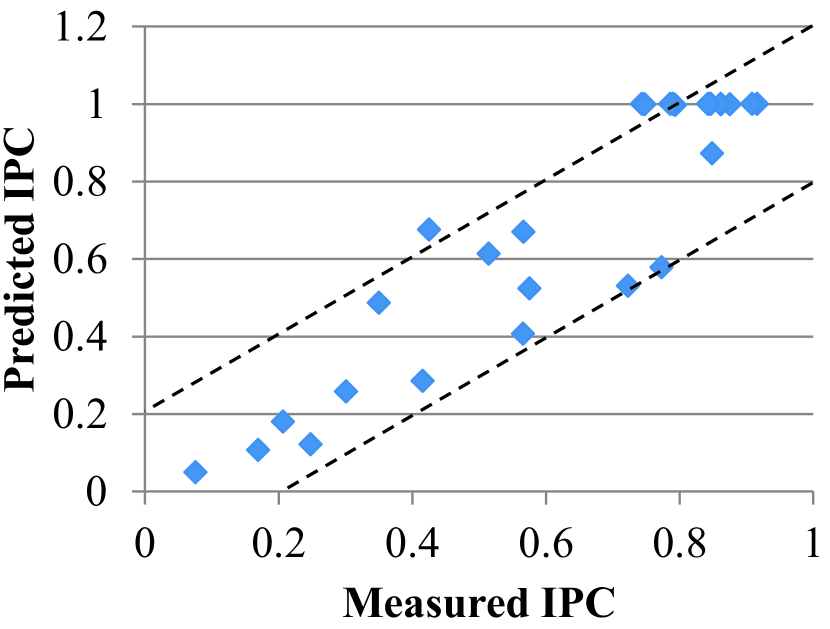
(a) C2050

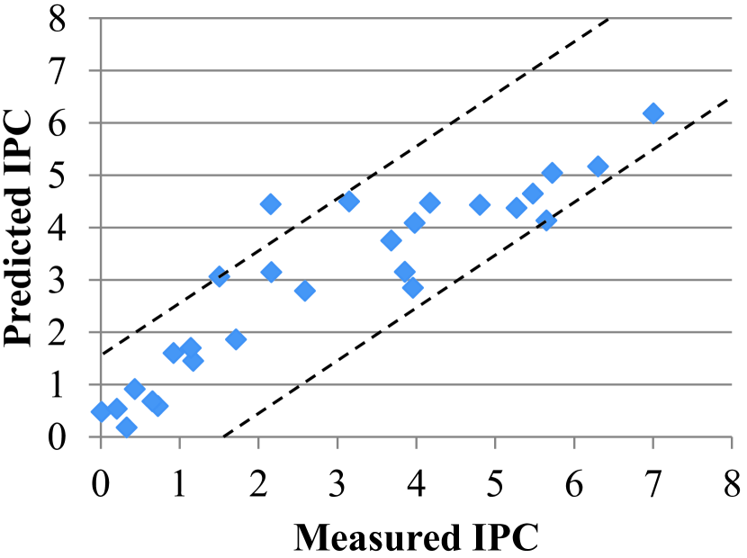
(b) GTX680

Figure 9: Comparison between predicted and measured concurrent kernel execution IPCs on two GPUs with fixed one-to-one slice ratio.

Model Optimizations. We further evaluate the impact of incorporating coalesced/uncoalesced memory accesses and the number of warp schedulers on the GPU. Only two applications (PC and SPMV) in our benchmark have uncoalesced memory accesses. We conduct the single kernel execution prediction experiments by (wrongly) assuming those two kernels with coalesced memory accesses only. The results are shown in Figure 10. Without considering uncoalesced access, the predicted IPC values are much larger than measurements since the assumption of coalesced access only underestimates the memory contention effects.

Figure 11 shows the results of concurrent execution IPC prediction on GTX680 without considering the multiple warp schedulers. The estimation without considering the number of warp schedulers severely underestimates the IPC on GTX680, in comparison with the results in Figure 8.

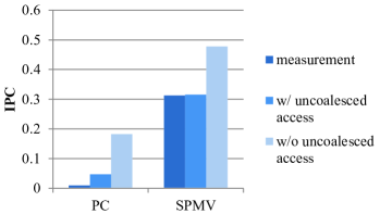
Figure 10: Comparison between predicted and measured concurrent kernel execution IPCs with/without considering uncoalesced access on C2050.

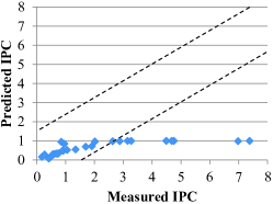
Figure 11: Comparison between predicted and measured concurrent kernel execution IPCs without considering multiple warp schedulers on GTX680.

$\mathit{CP}$ Prediction. We further evaluate the accuracy of $\mathit{CP}$ prediction. Figure 12 shows the comparison between measured and predicted $\mathit{CP}$ on C2050. We observe similar results on GTX680. The prediction is close to the measurement. With accurate prediction on $\mathit{IPC}$, the $\mathit{CP}$ difference between prediction and measurement is small. The results are sufficiently good to guide the scheduling decision as shown in the next section.

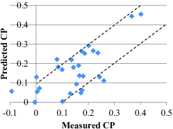
Figure 12: Comparison between predicted and measured ${CP}$ on C2050.

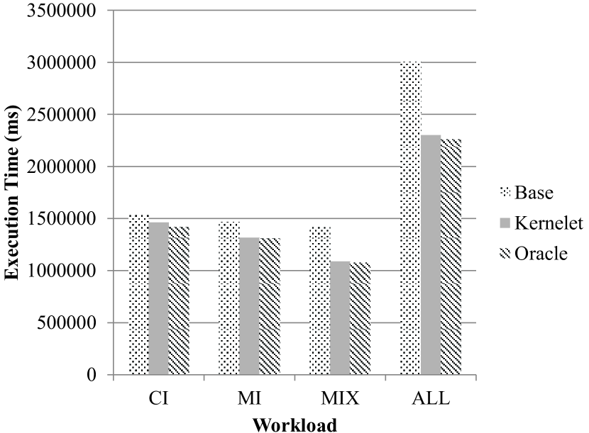
(a) C2050

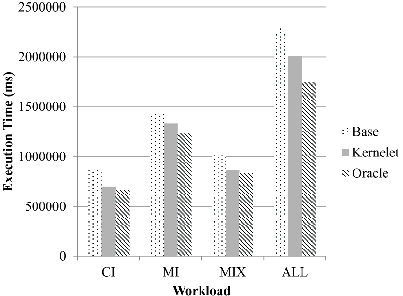
(b) GTX680

Figure 13: Comparison between different scheduling methods on both C2050 and GTX680.

5.4 Results on Kernel Scheduling

In this section, we evaluate the effectiveness of our kernel scheduling algorithm by comparing with BASE and OPT. To simulate the continuous kernel submission process, we initiate 1000 instances for each of each kernel mix and submit them for execution according to Poisson distributions. Different scheduling algorithms are applied and the total kernel execution time is reported. Figure 13 shows the total execution time of those kernels on C2050 and GTX680. On all the four workloads with different memory and computation characteristics, Kernelet outperforms Base (with the improvement 5.0–31.1% for C2050 and 6.7–23.4% for GTX680). Kernelet achieves similar performance to OPT (with the difference 0.7-3.1% for C2050 and 4.0–15.0% for GTX680). The performance improvement of Kernelet over Base is more significant on MIX and ALL, because Kernelet have more chances to select kernel pairs with complementary resource usage. Still, Kernelet outperforms Base in CI and MI, because slicing exposes the scheduling opportunities (even though they are small on CI and MI).

Table VI shows the number of kernels pruned with different pruning parameters $\alpha_{p}$ and $\alpha_{m}$ on C2050. Increasing $\alpha_{p}$ and $\alpha_{m}$ leads to more kernel combinations being pruned. Similar pruning result is oberserved for GTX680. Varying those two parameters can affect the pruning power and also the optimization opportunities. Thus, we choose the default values for $\alpha_{p}$ and $\alpha_{m}$ as 0.4 and 0.1 on C2050, and 0.4 and 0.105 on GTX680, respectively, as a tradeoff between pruning power and optimization opportunities.

TABLE VI: Number of kernels pruned with varying $\alpha_{p}$ and $\alpha_{m}$ on C2050.

	0.1	0.2	0.3	0.4	0.5	0.6	0.7	0.8	0.9	1.0
0.015	0	0	2	2	3	4	4	4	4	4
0.03	0	2	5	6	7	8	9	9	9	9
0.045	0	3	7	8	9	10	11	11	11	11
0.06	1	4	8	9	12	13	15	15	15	15
0.075	1	4	8	9	12	13	15	15	15	15
0.09	1	4	8	9	12	13	15	15	16	16
0.105	1	4	9	10	14	15	18	18	20	20
0.12	2	6	11	12	17	18	21	22	24	24
0.135	2	6	11	12	17	19	22	23	25	26
0.15	2	6	11	13	18	20	23	24	27	28

We finally study the execution time distribution of the scheduling candidate space. Figure 14 shows the CDF (cumulative distribution function) of the execution time of the MC($1000$). As we can see from the figure, none of the random schedules is better than Kernelet. It demonstrates that random co-schedules hurt the performance in a high probability due to the huge space of schedule plans.

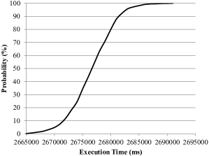
Figure 14: CDF (cumulative distribution function) of execution time of MC($1000$).

6 Related Work

In this section, we review the related work in two categories: 1) scheduling algorithms on CPUs, especially for CPUs with SMT (Simultaneous Multi-Threading), and 2) multi-kernel executions on GPUs.

6.1 CPU Scheduling and Performance Modeling

SMT has been an effective hardware technology to better utilize CPU resources. SMT allows instructions from multiple threads to be executed on the instruction pipeline at the same time. Various SMT aware scheduling techniques have been proposed to increase the CPU utilization[41, 39, 40, 24, 42, 8]. The core idea of SMT aware scheduling is to co-schedule threads with complementary resource requirements. Several mechanisms have been proposed to select the threads to be executed on the same SMT core, such as hardware counters feedback [41, 24], pre-execution of all combinations [39] and probabilistic job symbiosis model [8]. Performance models including the Markov chain based ones have also been adopted for concurrent tasks modeling on the CPUs. Serrano et al. [37, 36] developed a model to estimate the instruction throughput of super-scalar processors executing multiple instruction streams. Chen et al. [6] proposed an analytical model for estimating throughput of multi-threaded CPUs.

Despite the fruitful research results on SMT scheduling, they are not applicable to GPUs due to the architecture differences. First, main performance affecting issues are different for CPU and GPU applications. L2 data cache is a key consideration issue for SMT-aware thread scheduling, whereas thread parallelism is usually more important for the performance of GPGPU programs [2, 19, 38]. Second, scheduling on GPUs is not as flexible as that on CPUs. Current GPUs do not support task preemption. Third, unlike CPUs supporting the concurrent execution of a relatively small number of threads, each GPGPU kernel launches thousands of threads. Additionally, the maximum number of co-scheduling threads equals to the number of hardware context on the CPU, while the number of active warps on GPUs is dynamic, depending on the resource usage of the thread blocks. The slicing, scheduling and performance models in Kernelet are specifically designed for GPUs, taking those issues into consideration.

6.2 GPU Multiple Kernel Execution and Sharing

In the past few years, GPU architectures have undergone significant and rapid improvements for GPGPU support. Due to lack of concurrent kernel support in early GPU architectures, researchers initially proposed to merge two kernels at the source code level [14, 12]. In those methods, two kernels are combined into a single kernel with if-else branches on different granularities (e.g., thread blocks). They have three major disadvantages compared with our approach. First, combining the code of two kernels will increase the resource usage of each thread block, leading to lower SM occupancy and performance degradation [29]. Second, those approaches require source code, which may not be always available in the shared environments. Third, it requires two kernels with different block sizes avoiding using barriers within the thread block, otherwise deadlock may occur.

Recently, new-generation GPUs like NVIDIA Fermi GPUs support concurrent kernel executions. Taking advantage of this new capability, a number of multi-kernel optimization techniques [35, 15, 23] have been developed to improve the utilization of GPUs. Ravi et al. [34] proposed kernel consolidation to enable space sharing (different kernels run on different SMs) and time sharing (multiple kernels reside on the same SM) on GPUs. Space sharing happens when the total number of thread blocks of all kernels does not exceed the number of SMs and each block can be executed on a dedicated SM. If the total number of thread blocks is larger than the number of SMs, while SMs have sufficient resources to accommodate more thread blocks from different kernels, time sharing happens. That means, kernel consolidation does not have space sharing and have little time sharing when the launched kernels have sufficient thread blocks to occupy the GPU. Furthermore, they determined the kernel to be consolidated with heuristics based on the number of thread blocks. In contrast, Kernelet utilizes slicing to create more opportunities for time sharing, and develops a performance model to guide the scheduling decision. Peters et al. [32] used a persistently running kernel to handle requests from multiple applications. GPU virtualization has also been investigated [15, 23].

Recent studies also address the problem of GPU scheduling when multiple users co-reside in one machine. Pegasus [16] coordinates computing resources like accelerators and CPU and provides a uniform resource usage model. Timegraph [22] and PTask [35] manage the GPU at the operating system level. Kato et al. [21] introduced the responsive GPGPU execution model (RGEM). All those scheduling methods do not consider how to schedule concurrent kernels in order to fully utilize the GPU resources.

As for performance models on GPUs, Hong [19] and Kim [38] proposed analytical models based on the round-robin warp scheduling assumption. Baghsorkhi et al. [2] introduced the work flow graph interpretation of GPU kernels to estimate their execution time. All those models are designed for a single kernel. Moreover, they usually require extensive hardware profiling and/or simulation processes. In contrast, our performance model is designed for concurrent kernel executions on the GPU, and relies on a small set of key performance factors of individual kernel to predict the performance of concurrent kernel executions.

7 Conclusion

Recently, GPUs have been more and more widely used in clusters and cloud environments, where many kernels are submitted and executed on the shared GPUs. This paper proposes Kernelet to improve the throughput of concurrent kernel executions for such shared environments. Kernelet creates more sharing opportunities with kernel slicing, and uses a probabilistic performance model to capture the non-deterministic performance features of multiple-kernel executions. We evaluate Kernelet on two NVIDIA GPUs, Tesla C2050 and GTX680, with Fermi and Kepler architectures respectively. Our experiments demonstrate the accuracy of our performance model, and the effectiveness of Kernelet by improving the concurrent kernel executions by 5.0–31.1% and 6.7–23.4% on C2050 and GTX680 on our workloads, respectively.

References

- [1] asfermi: An assembler for the nvidia fermi instruction set. http://code.google.com/p/asfermi/, accessed on Dec 17th, 2012.
- [2] S. S. Baghsorkhi, M. Delahaye, S. J. Patel, W. D. Gropp, and W.-m. W. Hwu. An adaptive performance modeling tool for GPU architectures. SIGPLAN Not., 45(5):105–114, Jan. 2010.
- [3] S. S. Baghsorkhi, I. Gelado, M. Delahaye, and W.-m. W. Hwu. Efficient performance evaluation of memory hierarchy for highly multithreaded graphics processors. In Proc. of PPoPP ’12.
- [4] N. Bell and M. Garland. Cusp: Generic parallel algorithms for sparse matrix and graph computations version 0.3.0. http://cusp-library.googlecode.com, accessed on Dec 17th, 2012.
- [5] G. Chaitin. Register allocation & spilling via graph coloring. In ACM Sigplan Notices, volume 17, pages 98–105. ACM, 1982.
- [6] X. Chen and T. Aamodt. A first-order fine-grained multithreaded throughput model.
- [7] J. Duato, A. Pena, F. Silla, R. Mayo, and E. Quintana-Orti.
- [8] S. Eyerman and L. Eeckhout. Probabilistic job symbiosis modeling for smt processor scheduling. In Proc. of ASPLOS ’10.
- [9] M. Garland and D. B. Kirk. Understanding throughput-oriented architectures. Commun. ACM, 53(11), Nov. 2010.
- [10] N. Govindaraju, J. Gray, R. Kumar, and D. Manocha. GPUTeraSort: high performance graphics co-processor sorting for large database management. In Proc. of SIGMOD’06.
- [11] N. K. Govindaraju, B. Lloyd, Y. Dotsenko, B. Smith, and J. Manferdelli. High performance discrete fourier transforms on graphics processors. In ACM/IEEE SuperComputing ’08, 2008.
- [12] C. Gregg, J. Dorn, K. Hazelwood, and K. Skadron. Fine-grained resource sharing for concurrent GPGPU kernels. 0:389–398.
- [13] I. R. Group et al. Parboil benchmark suite, 2007.
- [14] M. Guevara, C. Gregg, K. Hazelwood, and K. Skadron. Enabling task parallelism in the cuda scheduler. In Workshop on Programming Models for Emerging Architectures (PMEA), 2009, page 69 C76.
- [15] V. Gupta, A. Gavrilovska, K. Schwan, H. Kharche, N. Tolia, V. Talwar, and P. Ranganathan. Gvim: GPU-accelerated virtual machines. In Proceedings of the 3rd ACM Workshop on System-level Virtualization for High Performance Computing, HPCVirt ’09, pages 17–24, New York, NY, USA, 2009. ACM.
- [16] V. Gupta, K. Schwan, N. Tolia, V. Talwar, and P. Ranganathan. Pegasus: coordinated scheduling for virtualized accelerator-based systems. In Proc. of USENIXATC’11.
- [17] B. He, M. Lu, K. Yang, R. Fang, N. K. Govindaraju, Q. Luo, and P. V. Sander. Relational query coprocessing on graphics processors. ACM Trans. Database Syst., 34(4):1–39, 2009.
- [18] B. He, K. Yang, R. Fang, M. Lu, N. Govindaraju, Q. Luo, and P. Sander. Relational joins on graphics processors. In Proc. of SIGMOD ’08.
- [19] S. Hong and H. Kim. An analytical model for a GPU architecture with memory-level and thread-level parallelism awareness. In Proc. of ISCA’09.
- [20] Y. Jiang, X. Shen, J. Chen, and R. Tripathi. Analysis and approximation of optimal co-scheduling on chip multiprocessors. In Proc. of PACT’08.
- [21] S. Kato, K. Lakshmanan, A. Kumar, M. Kelkar, Y. Ishikawa, and R. R. Rajkumar. Rgem: A responsive gpgpu execution model for runtime engines. In Proc. of RTSS’11.
- [22] S. Kato, K. Lakshmanan, R. Rajkumar, and Y. Ishikawa. TimeGraph: GPU scheduling for real-time multi-tasking environments. In Proc. of USENIXATC’11.
- [23] T. Li, V. Narayana, E. El-Araby, and T. El-Ghazawi. In Proc. of ICPP’11.
- [24] T. Moseley, D. Grunwald, J. L. Kihm, and D. A. Connors. Methods for modeling resource contention on simultaneous multithreading processors. In Proc. of ICCD’05.
- [25] R. Nath, S. Tomov, T. T. Dong, and J. Dongarra. Optimizing symmetric dense matrix-vector multiplication on GPUs. In Proc. of SC’11.
- [26] A. Nukada, Y. Ogata, T. Endo, and S. Matsuoka. Bandwidth intensive 3-D FFT kernel for gpus using cuda. In Proc. of SC’08.
- [27] NVIDIA. NVIDIA Fermi Compute Architecture Whiltepaper, v1.1 edition.
- [28] NVIDIA. NVIDIA GeForce GTX 680 Whiltepaper, v1.0 edition.
- [29] NVIDIA. NVIDIA CUDA C Programming Guide 4.2, 2012.
- [30] NVIDIA CUDA. http://developer.nvidia.com/object/cuda.html.
- [31] A. Papoulis and R. Probability. Stochastic processes, volume 3. McGraw-hill New York, 1991.
- [32] H. Peters, M. Koper, and N. Luttenberger. Efficiently using a CUDA-enabled GPU as shared resource. In Proc. of CIT’10.
- [33] M. Poletto and V. Sarkar. Linear scan register allocation. ACM Transactions on Programming Languages and Systems (TOPLAS), 21(5):895–913, 1999.
- [34] V. T. Ravi, M. Becchi, G. Agrawal, and S. Chakradhar. Supporting GPU sharing in cloud environments with a transparent runtime consolidation framework. In Proc. of HPDC’11.
- [35] C. J. Rossbach, J. Currey, M. Silberstein, B. Ray, and E. Witchel. PTask: operating system abstractions to manage gpus as compute devices. In Proc. of SOSP’11.
- [36] M. Serrano. Performance estimation in a simultaneous multithreading processor. In Proc. of MASCOTS’96.
- [37] M. Serrano, W. Yamamoto, R. Wood, and M. Nemirovsky. A model for performance estimation in a multistreamed superscalar processor. In Computer Performance Evaluation Modelling Techniques and Tools, volume 794 of Lecture Notes in Computer Science, pages 213–230. 1994.
- [38] J. Sim, A. Dasgupta, H. Kim, and R. Vuduc. A performance analysis framework for identifying potential benefits in GPGPU applications. In Proc. of PPoPP’12.
- [39] A. Snavely and D. M. Tullsen. Symbiotic jobscheduling for a simultaneous multithreaded processor. In Proceedings of the ninth international conference on Architectural support for programming languages and operating systems, ASPLOS-IX, 2000.
- [40] A. Snavely, D. M. Tullsen, and G. Voelker. Symbiotic jobscheduling with priorities for a simultaneous multithreading processor. In Proc. of SIGMETRICS’02.
- [41] S. E. Sujay Parekh and H. Levy. Thread-sensitive scheduling for SMT processors. Technical report 2000-04-02, University of Washington.
- [42] D. Tam, R. Azimi, and M. Stumm. Thread clustering: sharing-aware scheduling on smp-cmp-smt multiprocessors. In Proceedings of the 2nd ACM SIGOPS/EuroSys European Conference on Computer Systems 2007, EuroSys ’07, 2007.
- [43] V. Volkov and J. W. Demmel. Benchmarking GPUs to tune dense linear algebra. In Proc. of SC’08.
- [44] Y. Zhang and J. D. Owens. A quantitative performance analysis model for gpu architectures. In Proc. of HPCA’11, 2011.
- [45] Zillians. V-GPU: GPU virtualization. http://www.zillians.com/products/vgpu-gpu-virtualization/, accessed on Dec 17th, 2012.