Invisible decays of ultra-high energy neutrinos

L. Dorame^a, O. G. Miranda^b, J. W. F. Valle^a
aAHEP Group, Institut de Física Corpuscular – C.S.I.C./Universitat de València, Valencia, Spain
^bDepartamento de Física, Centro de Investigación y de Estudios Avanzados del IPN México, DF, Mexico

Abstract
Gamma-ray bursts (GRBs) are expected to provide a source of ultra high energy cosmic rays, accompanied with potentially detectable neutrinos at neutrino telescopes. Recently, IceCube has set an upper bound on this neutrino flux well below theoretical expectation. We investigate whether this mismatch between expectation and observation can be due to neutrino decay. We demonstrate the phenomenological consistency and theoretical plausibility of the neutrino decay hypothesis. A potential implication is the observability of majoron-emitting neutrinoless double beta decay.

The source of ultra high energy cosmic rays remains a mystery. In gamma-ray burst (GRB) models such as the fireball model cosmic-ray acceleration should be accompanied by neutrinos produced in the decay of charged pions created in interactions between the high-energy protons and $\gamma$-rays [1]. Recently the Ice-Cube collaboration reported an upper limit on the flux of energetic neutrinos associated with GRBs almost four times below this prediction [2].

Various possible explanations have been considered to explain the non observation of this ultra high energy neutrino flux. For example, a complete detailed numerical analysis of the fireball neutrino model predicts a neutrino flux that is one order of magnitude lower than the analytical computations [3]. On the other hand, another recent computation [4] of the neutrino flux in the fireball model gives a mild reduction in the neutrino flux if a relation between the bulk Lorentz factor, $\Gamma$, and the burst energy is assumed. Finally, based on the specific case of GRB 130427A, it has been argued that the low neutrino flux can be explained with relatively large values for the bulk Lorentz factor ($\Gamma\geq 500$) and for the dissipation radius ($R_{d}\geq 10^{14}$ cm); it was shown in the same reference that both the internal shock and the baryon photosphere models satisfied these conditions.

Here we focus on a different approach to explain the neutrino flux deficit. Instead of studying the astrophysical mechanism of the source objects, we look for a high energy physics explanation. Some mechanisms involving new physics in order to explain a possible deficit in the observed neutrino flux have already been suggested. For instance, the possibility of an oscillations involving a quasi Dirac neutrino [5] has been considered in Ref. [6]; a specific model for this case has been studied in [7] and the possibility of a resonance effect has also been discussed [8]. Another mechanism recently discussed has been the case of a spin precession into a sterile neutrino as a result of a nonzero neutrino magnetic moment [9] and the strong magnetic fields expected to be present in a GRB [10].

Here we speculate on the plausibility of the neutrino decay hypothesis as a possible explanation for the mismatch between observation and expectation. The most attractive possibility involves invisible decays, which have been considered theoretically since the eighties [17, 11, 12, 13, 14], and recently revisited for the case of GRB neutrino fluxes [15]. These decays arise in models with spontaneous violation of ungauged lepton number [16], though typically suppressed [17]. A natural scenario to test neutrino stability are astrophysical objects [18, 19, 20, 21]. In particular, limits on Majoron couplings from solar and supernova neutrinos have been obtained in Refs. [22]. For non astrophysical constraints, for example from $0\nu\beta\beta$ searches, see [23, 24, 25, 26]. Moreover, as already mentioned, recent results from the Pierre Auger Observatory (PAO) [27], ANTARES [28] and IceCube [29] have placed strong constraints on the neutrino flux coming from distant ultra high energy (UHE) neutrino sources.

Here we explore the phenomenological plausibility and theoretical consistency of the decay hypothesis within a class of low-scale $\mathrm{SU(3)_{c}\otimes SU(2)_{L}\otimes U(1)_{Y}}$ seesaw schemes with spontaneous family-dependent lepton number violation. We show that the required neutrino decay lifetime range hinted by the non observation of UHE muon neutrinos is theoretically achievable for the majoron-emitting neutrino decays and, moreover, consistent with all existing phenomenological constraints.

The decay rate $\nu_{i}\to\nu_{j}+J$ in the rest frame of $\nu_{i}$ is

$$\Gamma(\nu_{i}\to\nu_{j}+J)=\dfrac{g_{ij}^{2}}{16\pi}\dfrac{(m_{i}+m_{j})^{2}}{m_{i}^{3}}(m_{i}^{2}-m_{j}^{2})\ \ ,$$ (1)

where $\nu_{i}$ and $\nu_{j}$ are active neutrinos and $J$ is a massless or very light majoron associated to the spontaneous violation of ungauged lepton number. Taking $m_{j}=0$, we can estimate the decay length (in meters) for a relativistic neutrino as given by

$$L=c\tau=\dfrac{cE_{i}}{m_{i}\Gamma}\simeq 1\times 10^{9}\left(g_{ij}^{-2}\right)\left(\dfrac{E_{i}}{100\mbox{TeV}}\right)\left(\dfrac{1\mbox{eV}}{m_{i}}\right)^{2}\mbox{m}.$$ (2)

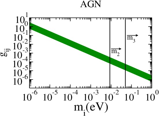
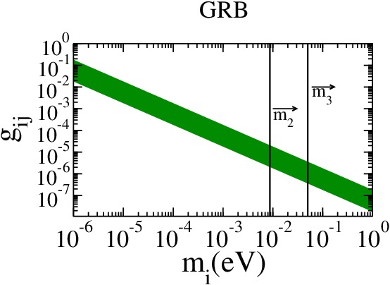
For typical AGN distances we obtain the required values of $g_{ij}$ for a given neutrino mass $m_{i}$ which would cause decay before reaching the detector. In Fig. (1) we took AGN distances from $3.6$ Mpc (the distance to Centaurus A) up to $100$ Mpc. In the bottom panel of the same Fig. (1) we have plotted the corresponding result for GRBs, at typical distances of $10$ - $10^{3}$ Mpc. The vertical lines correspond to the relevant region for $m_{2}$ and $m_{3}$ for the case $m_{1}=0$. We have explicitly verified that, for the GRB case, this approximation is in agreement with more detailed estimates of neutrino lifetime ranges [30].

As we will discuss below, putting into a theory context, such couplings are fairly large to achieve theoretically.

Figure 1: Neutrino mass $m_{i}$ versus the required coupling constant $g_{ij}$ for the case of AGN’s (left panel) and GRBs (right panel).

In order to have an estimate of the neutrino flux reduction resulting from neutrino decay we note that, since coherence is lost, the final flux of a given neutrino flavour will be

$$\phi_{\nu_{\alpha}}(E)=\sum_{i\beta}\phi_{\nu_{\beta}}^{\rm source}(E)|U_{\beta i}|^{2}|U_{\alpha i}|^{2}e^{-L/\tau_{i}(E)},$$ (3)

where $\phi$’s are neutrino fluxes at production and detection, L the travel distance, $\tau_{i}$ the neutrino lifetime in the laboratory frame and $U_{\alpha i}$ the elements of the lepton mixing matrix [31]. Typical neutrino energies lie in the range of $10^{5}$ TeV and $10^{3}$ TeV for AGNs and GRBs respectively. Note that, in the limit that $L\gg\tau_{i}$ where only the stable state survives Eq. (3) becomes

$$\phi_{\nu_{\alpha}}(E)=\sum_{i(\rm stable)\beta}\phi_{\nu_{\beta}}^{\rm source}(E)|U_{\beta i}|^{2}|U_{\alpha i}|^{2}.$$ (4)

Here we take a normal hierarchy neutrino mass spectrum, the disappearance of all states except the lightest (in this case $\nu_{1}$) is allowed. The final flux of $\nu_{e}$, $\nu_{\mu}$ and $\nu_{\tau}$ can be computed from Eq. (4) and will depend on the three mixing angles and the Dirac CP phase $\delta$. In particular, we can calculate the suppression of the muon neutrino flux, $\phi_{\nu_{\mu}}$, using the ratio

$$R_{\nu_{e}:\nu_{\mu}}\equiv\dfrac{\phi_{\nu_{e}}}{\phi_{\nu_{\mu}}}=\left(\dfrac{\cos{\theta_{12}}\cos{\theta_{13}}}{|-\sin{\theta_{12}}\cos{\theta_{23}}-\sin{\theta_{13}}\sin{\theta_{23}}\cos{\theta_{12}}e^{\imath\delta}|}\right)^{2},$$ (5)

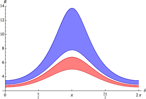
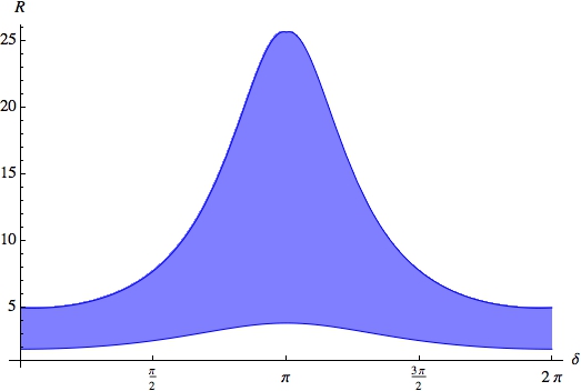
where $\theta_{12}$, $\theta_{23}$ and $\theta_{13}$ are the neutrino mixing angles determined in neutrino oscillation experiments. The left panel of Fig. (2) shows the expected values for this ratio when the neutrino mixing angles lie within the $1\sigma$ bands from their current global best fit values [32, 33, 34] One can also see, in the right panel of the same Fig. (2), that by allowing these parameters to vary up to their three sigma ranges, $R_{\nu_{e}:\nu_{\mu}}$ can be as large as 25 or as low as 2. Very similar results are found for global fit of Ref. [33], as shown in Table 1.

Global Fit	$1^{st}$octant	$2^{nd}$octant	At $3\sigma$
Forero, et. al. [32]	2-7	3-14	2-25
González-García, et. al. [33]	2-7	3-12	2-23
Fogli, et. al. [34]	2-6	-	2-22

Table 1: Allowed values of $R_{\nu_{e}:\nu_{\mu}}$ according to different neutrino oscillation fits. The second column shows the allowed region for the case of a $\theta_{23}$ in the first octant, while the third column shows the second octant case. Finally, the fourth column displays the allowed region if we consider the 3 $\sigma$ confidence level for $\theta_{23}$.

It is important to notice that, in this picture, the neutrino decay will lead to a decrease in the muon neutrino flux while the electron neutrino flux will increase. Alternatively in the presence of light sterile states one can envisage a scenario where the muon neutrino decays to the sterile state. Here we do not consider this case. Recent data from Icecube reports the observation of two neutrinos with energies around $10^{15}$ eV, probably electron neutrinos [35]. Moreover, there have been recent announcements of more neutrino events detected in IceCube [36].

Figure 2: $R_{\nu_{e}:\nu_{\mu}}$ versus the CP phase $\delta$ for neutrino mixing angles [32] at 1$\sigma$ (left panel) and at 3$\sigma$ (right panel). For the 1$\sigma$ case we show two regions: one for $\theta_{23}$ in the $1^{st}$ octant (orange lower band) and another one for $\theta_{23}$ in the $2^{nd}$ octant (blue higher band). One can see that values of $\theta_{23}$ in the $2^{nd}$ octant give a stronger effect.

We now turn to the issue of theoretical consistency of the decay hypothesis. In most $\mathrm{SU(3)_{c}\otimes SU(2)_{L}\otimes U(1)_{Y}}$ seesaw models with spontaneous lepton number violation when one diagonalizes the neutrino mass matrix one also diagonalizes, to first approximation, the coupling of the resulting Nambu-Goldstone boson to the mass eigenstate neutrinos [17]. The exact form of the light-neutrino majoron couplings can be determined explicitly by perturbative diagonalization of the seesaw mass matrix, or by using a more general approach using only the symmetry properties. The result is [17]

$${g}_{ij}=-\frac{m_{i}}{v_{1}}\delta_{ij}+\left[\frac{m_{i}}{v_{1}}\left(V_{1}^{\dagger}D^{*}{M}^{*-1}{M}^{-1}D^{T}V_{1}\right)_{ij}\right]_{\rm S}+\ldots$$ (6)

where the subscript S denotes symmetrization, $D$ and $M$ are the Dirac and Majorana mass terms in, say, the type-I seesaw scheme and $V_{1}$ is the light neutrino diagonalization matrix. One sees that the majoron couples proportionally to the light neutrino mass, hence the coupling matrix is diagonal to first approximation. The off-diagonal part of the $g_{ij}$ is inversely proportional to three powers of lepton number violation scale $v_{1}\equiv\left\langle\sigma\right\rangle$, since $M\propto v_{1}$. This is tiny, the only hope being to use a seesaw scheme that allows for a very low lepton number violation scale, such as the inverse seesaw [37]. The particle content is the same as that of the Standard Model (SM) except for the addition of a pair of two component gauge singlet leptons, $\nu^{c}_{i}$ and $S_{i}$, within each of the three generations, labeled by $i$. The isodoublet neutrinos $\nu_{i}$ and the fermion singlets $S_{i}$ have the same lepton number, opposite with respect to that of the three singlets $\nu^{c}_{i}$ associated to the “right-handed” neutrinos. In the $\nu$, $\nu^{c}$, $S$ basis the $9\times 9$ neutral lepton mass matrix $M_{\nu}$ has the form:

$$M_{\nu}=\left[\begin{array}[]{ccc}0&m_{D}^{T}&0\\ m_{D}&0&M^{T}\\ 0&M&\mu\end{array}\right],$$ (7)

where $m_{D}\propto\left\langle\Phi\right\rangle$ is the standard Dirac term coming from the SM Higgs vev and $M$ is a bare mass term. The term $\mu\propto\left\langle\sigma\right\rangle$, the vacuum expectation value of $\sigma$ responsible for spontaneous low-scale lepton number violation as proposed in [14]. This gives rise to a majoron J,

$$J=\sqrt{2}\ \mbox{Im}\sigma.$$ (8)

As a result of diagonalization one obtains an effective light neutrino mass matrix. Note that lepton number symmetry is recovered as $\mu\to$ 0, making the three light neutrinos strictly massless. The majoron couplings of the light mass eigenstate neutrinos are determined again as a sum of two pieces as in Eq. (6). Detailed calculation shows that its off-diagonal part behaves as $P^{\prime}\sim\mu^{2}D^{2}{M}^{-4}$. Even if the $M$ can be significantly lower than that of the standard high-scale type-I seesaw it is clear that this is way too small in order to produce neutrino decay within the relevant astrophysical scales.

The only way out is to induce a mismatch between the neutrino mass basis and the coupling basis. This can be achieved by making lepton number a family-dependent symmetry [12, 13]. The model is by no means unique, here we give an example based on $\mathrm{SU(3)_{c}\otimes SU(2)_{L}\otimes U(1)_{Y}}$ $\otimes U(1)_{H}$ assigned as shown in Table 2

	$\overline{L_{e}}$	$\overline{L_{\mu}}$	$\overline{L_{\tau}}$	$\nu_{R_{e}}$	$\nu_{R_{\mu}}$	$\nu_{R_{\tau}}$	$h$	$S_{1}$	$S_{2}$	$S_{3}$	$\sigma$
$SU(2)$	2	2	2	1	1	1	2	1	1	1	1
$U(1)_{H}$	$-2$	$-2$	$-4$	$2$	$2$	4	0	$0$	$0$	$-2$	$-2$

Table 2: Model field representation content and transformation properties

The $\mathrm{SU(3)_{c}\otimes SU(2)_{L}\otimes U(1)_{Y}}$ $\otimes U(1)_{H}$ invariant Lagrangian would be

$$\mathcal{L}_{\nu}=m_{D_{ij}}\bar{L_{i}}\nu_{R_{j}}h+{M_{ij}}\bar{\nu}^{c}_{R_{i}}S_{j}+$$ (9)

$$M_{\sigma_{ij}}\bar{\nu}^{c}_{R_{i}}S_{j}\sigma+\mu_{ij}\bar{S}_{i}S_{j}+{\mu_{\sigma_{ij}}}\bar{S}_{i}S_{j}\sigma^{*}+h.c.,$$

where the relevant sub-matrices are

$$m_{D}=\left[\begin{array}[]{ccc}m_{a}&m_{b}&0\\ m_{c}&m_{d}&0\\ 0&0&m_{e}\end{array}\right],\quad M=\left[\begin{array}[]{ccc}0&0&M_{1}\\ 0&0&M_{2}\\ 0&0&0\end{array}\right],$$ (16)

$$M_{\sigma}=\left[\begin{array}[]{ccc}M_{3}&M_{4}&0\\ M_{5}&M_{6}&0\\ 0&0&M_{7}\end{array}\right]$$ (20)

$$\mu=\left[\begin{array}[]{ccc}M_{8}&M_{9}&0\\ M_{10}&M_{11}&0\\ 0&0&0\end{array}\right],\quad\mu_{\sigma}=\left[\begin{array}[]{ccc}0&0&M_{12}\\ 0&0&M_{13}\\ M_{14}&M_{15}&0\end{array}\right]$$ (21)

One can check explicitly that the first term in Eq. (6) is already non-diagonal and, for sufficiently low values of the $U(1)_{H}$ breaking scale can induce a decay sufficiently fast as to suppress the flux of $\phi_{\nu_{\mu}}$ to account for its non observation of $\nu_{\mu}$ by Ice Cube.

As an additional interesting feature of this scheme, we propose an indirect test of our neutrino decay hypothesis through the single majoron-emitting $J0\nu\beta\beta$ decay mode [38]

$$(A,Z)\rightarrow(A,Z+2)+2\,e^{-}+J.$$ (22)

The decay rate for single Majoron emission is given by [39]

$$\Gamma^{0\nu}=\left|\left\langle g_{ee}\right\rangle\right|^{2}\left|{\mathcal{M}}_{J}\right|^{2}\,G_{J}(Q,Z)\,,$$ (23)

where $\left|\left\langle g_{ee}\right\rangle\right|$ is an averaged coupling constant, $G_{J}(Q,Z)$ accounts for the phase space factor and the nuclear matrix element (NME) ${\mathcal{M}}_{J}$ depends on the mechanism and the relevant nucleus. For single Majoron emission one can use the same NMEs from the standard $0\nu\beta\beta$ decay [40].

Figure 3: Left panel: Single majoron-emitting $J0\nu\beta\beta$ coupling $\left\langle g_{ee}\right\rangle$ versus $\left\langle g_{12}\right\rangle$, when varying the values of the neutrino mass terms, for the best fit values of the neutrino mixing angles and $\delta=0$. Right panel: Correlation between $R_{\nu_{e}:\nu_{\mu}}$ and the parameter $\left\langle g_{ee}\right\rangle$ for two particular points of the left panel, varying in this case the value of $\delta$

.

We can see from Eq. (23) that the decay width for single Majoron emission in neutrinoless double beta decay depends on the coupling constant $g_{ee}$ and it is therefore an indirect relation with the expression in Eq. (1) through the coupling $g_{12}$.

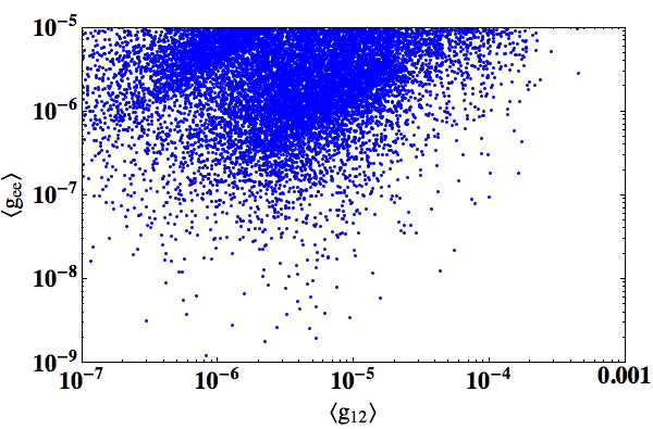
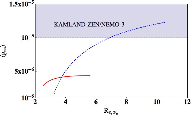
Indeed if the majoron exists and its coupling to the electron neutrino is not expected to significantly differ from the one required to explain the muon neutrino deficit in IceCube through the neutrino decay hypothesis, there will be a correlation between $R_{\nu_{e}:\nu_{\mu}}$ and $\left\langle g_{ee}\right\rangle$. This correlation is depicted in Fig. 3. We plot in the left panel the correspondence between $g_{ee}$ and $g_{12}$ when we fix the neutrino mixing angles at their best fit values and we consider a Dirac mass entry at $m_{D}\sim$ 10 GeV, $M\sim$ 1 TeV $M_{\sigma}\sim$ 1 TeV and $\mu\sim$ 1 keV where the $\sim$ sign takes into account order one differences among the various flavour components of each block. In the right panel of the same figure, we take one the of the points shown in the left panel and vary its CP phase from 0 to $2\pi$ in order to obtain an estimate for the ratio $R_{\nu_{e}:\nu_{\mu}}$ relevant at IceCube. The dotted (blue) curve corresponds to the case when we consider the second octant of the atmospheric mixing angle, particularly its central value $\sin^{2}\theta_{23}=0.61$ (we have also chosen the central values of the other mixing angles, $\sin^{2}\theta_{12}=0.320$ and $\sin^{2}\theta_{13}=0.0246$); from this case it is possible to see that, for example, for a coupling constant $\left\langle g_{ee}\right\rangle=4.33\times 10^{-6}$ a reduction by a factor five in the muon flux can be obtained for an appropriate value of the $CP$ phase, $\delta=2.5$, while the suppression could be as high as a factor $10$. The solid (red) line corresponds to a point in the first octant ($\sin^{2}\theta_{23}=0.427$). Although in this particular case the values of the ratio, $R_{\nu_{e}:\nu_{\mu}}$ are lower than for the second octant, one can still achieve an important suppression; in particular, we can see that a reduction by a factor five is again possible (for the values $\left\langle g_{ee}\right\rangle=7.34\times 10^{-6}$ and $\delta=1.6$) This is an interesting observation, considering that currently the “preferred” octant is not yet uniquely determined by the neutrino oscillation fits [33, 34, 32]. Moreover, we can see that even with the central values of the neutrino mixing angles one can obtain a suppression factor of five or higher, that could be sufficient to explain the limits reported by the IceCube collaboration [2].

In conclusion one sees that the decay hypothesis invoked to account for the IceCube results may be tested in the upcoming searches for the $J0\nu\beta\beta$ decay.

Work supported by MINECO grants FPA2011-22975 and MULTIDARK Consolider CSD2009-00064, by Prometeo/2009/091 (Gen. Valenciana), and by EPLANET. L. D. is supported by JAE Predoctoral fellowship. O. G. M. was supported by CONACyT grant 132197.

References

- [1] E. Waxman and J. N. Bahcall, Phys. Rev. Lett. 78, 2292 (1997) [astro-ph/9701231].
- [2] R. Abbasi et al. [IceCube Collaboration], Nature 484, 351 (2012) [arXiv:1204.4219 [astro-ph.HE]].
- [3] S. Hummer, P. Baerwald and W. Winter, Phys. Rev. Lett. 108, 231101 (2012) [arXiv:1112.1076 [astro-ph.HE]].
- [4] H. -N. He, R. -Y. Liu, X. -Y. Wang, S. Nagataki, K. Murase and Z. -G. Dai, Astrophys. J. 752, 29 (2012) [arXiv:1204.0857 [astro-ph.HE]].
- [5] J. W. F. Valle, Phys. Rev. D 27, 1672 (1983).
- [6] A. Esmaili and Y. Farzan, JCAP 1212, 014 (2012) [arXiv:1208.6012 [hep-ph]].
- [7] A. S. Joshipura, S. Mohanty and S. Pakvasa, arXiv:1307.5712 [hep-ph].
- [8] O. G. Miranda, C. A. Moura and A. Parada, arXiv:1308.1408 [hep-ph].
- [9] J. Schechter and J. W. F. Valle, Phys. Rev. D 24, 1883 (1981) [Erratum-ibid. D 25, 283 (1982)].
- [10] J. Barranco, O. G. Miranda, C. A. Moura and A. Parada, Phys. Lett. B 718, 26 (2012) [arXiv:1205.4285 [astro-ph.HE]].
- [11] J. W. F. Valle, Phys. Lett. B 131, 87 (1983).
- [12] G. B. Gelmini and J. W. F. Valle, Phys. Lett. B 142, 181 (1984).
- [13] G. Gelmini, D. N. Schramm and J. W. F. Valle, Phys. Lett. B 146, 311 (1984).
- [14] M. C. Gonzalez-Garcia and J. W. F. Valle, Phys. Lett. B 216, 360 (1989).
- [15] S. Pakvasa, A. Joshipura and S. Mohanty, arXiv:1209.5630 [hep-ph].
- [16] Y. Chikashige, R. N. Mohapatra and R. D. Peccei, Phys. Lett. B 98, 265 (1981).
- [17] J. Schechter and J. W. F. Valle, Phys. Rev. D 25, 774 (1982).
- [18] J. N. Bahcall, S. T. Petcov, S. Toshev and J. W. F. Valle, Phys. Lett. B 181, 369 (1986).
- [19] P. Keranen, J. Maalampi and J. T. Peltoniemi, Phys. Lett. B 461, 230 (1999) [hep-ph/9901403].
- [20] J. F. Beacom and N. F. Bell, Phys. Rev. D 65, 113009 (2002) [hep-ph/0204111].
- [21] J. F. Beacom, N. F. Bell, D. Hooper, S. Pakvasa and T. J. Weiler, Phys. Rev. Lett. 90, 181301 (2003) [hep-ph/0211305].
- [22] M. Kachelriess, R. Tomas and J. W. F. Valle, Phys. Rev. D 62, 023004 (2000) [hep-ph/0001039].
- [23] R. Tomas, H. Pas and J. W. F. Valle, Phys. Rev. D 64, 095005 (2001) [hep-ph/0103017].
- [24] A. P. Lessa and O. L. G. Peres, Phys. Rev. D 75, 094001 (2007) [hep-ph/0701068].
- [25] A. Gando et al. [KamLAND-Zen Collaboration], Phys. Rev. C 86, 021601 (2012) [arXiv:1205.6372 [hep-ex]].
- [26] J. Argyriades et al. [NEMO-3 Collaboration], Nucl. Phys. A 847, 168 (2010) [arXiv:0906.2694 [nucl-ex]].
- [27] P. Abreu et al. [Pierre Auger Collaboration], arXiv:1107.4805 [astro-ph.HE].
- [28] S. Biagi, Nucl. Phys. Proc. Suppl. 212-213, 109 (2011) [arXiv:1101.3670 [astro-ph.HE]].
- [29] R. U. Abbasi, T. Abu-Zayyad, M. Allen, J. F. Amann, G. Archbold, K. Belov, J. W. Belz and S. Y. B. Zvi et al., arXiv:0803.0554 [astro-ph].
- [30] P. Baerwald, M. Bustamante and W. Winter, JCAP 1210, 020 (2012) [arXiv:1208.4600 [astro-ph.CO]].
- [31] J. Schechter and J. W. F. Valle, Phys. Rev. D 22, 2227 (1980).
- [32] D. V. Forero, M. Tortola and J. W. F. Valle, Phys. Rev. D 86, 073012 (2012) [arXiv:1205.4018 [hep-ph]].
- [33] M. C. Gonzalez-Garcia, M. Maltoni, J. Salvado and T. Schwetz, JHEP 1212, 123 (2012) [arXiv:1209.3023 [hep-ph]].
- [34] G. L. Fogli, E. Lisi, A. Marrone, D. Montanino, A. Palazzo and A. M. Rotunno, Phys. Rev. D 86, 013012 (2012) [arXiv:1205.5254 [hep-ph]].
- [35] M. G. Aartsen et al. [IceCube Collaboration], Phys. Rev. Lett. 111, 021103 (2013) [arXiv:1304.5356 [astro-ph.HE]].
- [36] N. Whitehorn, C. Kopper, and N. K. Neilson, talk given at the IceCube Particle Astrophysics Symposium (IPA) 2013, Madison, WI, USA.
- [37] R. N. Mohapatra and J. W. F. Valle, Phys. Rev. D 34, 1642 (1986).
- [38] H. M. Georgi, S. L. Glashow and S. Nussinov, Nucl. Phys. B 193, 297 (1981).
- [39] W. Rodejohann, Int. J. Mod. Phys. E 20, 1833 (2011) [arXiv:1106.1334 [hep-ph]].
- [40] M. Hirsch, H. V. Klapdor-Kleingrothaus, S. G. Kovalenko and H. Pas, Phys. Lett. B 372, 8 (1996) [hep-ph/9511227].