Parameter estimation for pair-copula constructions

Abstract

We explore various estimators for the parameters of a pair-copula construction (PCC), among those the stepwise semiparametric (SSP) estimator, designed for this dependence structure. We present its asymptotic properties, as well as the estimation algorithm for the two most common types of PCCs. Compared to the considered alternatives, that is, maximum likelihood, inference functions for margins and semiparametric estimation, SSP is in general asymptotically less efficient. As we show in a few examples, this loss of efficiency may however be rather low. Furthermore, SSP is semiparametrically efficient for the Gaussian copula. More importantly, it is computationally tractable even in high dimensions, as opposed to its competitors. In any case, SSP may provide start values, required by the other estimators. It is also well suited for selecting the pair-copulae of a PCC for a given data set.

1 Introduction

The last decades’ technological revolution have considerably increased the relevance of multivariate modelling. Copulae are now regularly used within fields such as finance, survival analysis and actuarial sciences. Although the list of parametric bivariate copulae is long and varied, the choice is rather limited in higher dimensions (Genest et al. [15]). Accordingly, a number of hierarchical, copula-based structures have been proposed, among those the pair-copula construction (PCC) of Joe [22], further studied and considered by Bedford and Cooke [2, 3], Kurowicka and Cooke [30] and Aas et al. [1].

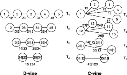
A PCC is a treelike construction, built from pair-copulae with conditional distributions as their two arguments (see Figure 1). The number of conditioning variables is zero at the ground, and increases by one for each level, to ensure coherence of the construction. Despite its simple structure, the PCC is highly flexible and covers a wide range of complex dependencies (Joe et al. [25], Hobæk Haff et al. [21]). After Aas et al. [1] set it in an inferential context, it has made several appearances in the literature (Fischer et al. [13], Chollete et al. [6], Heinen and Valdesogo [19], Schirmacher and Schirmacher [35], Czado and Min [9], Kolbjørnsen and Stien [29], Czado et al. [10, 11]), exhibiting its adequacy for various applications.

Regardless of its recent popularity, estimation of PCC parameters has so far been addressed mostly in an applied setting. The aim of this work is to explore the properties of alternative estimators. As the PCC is a member of the multivariate copula family, one may exploit the large collection of estimators proposed for that model class, such as moments type procedures, based on, for instance, the matrix of pairwise Kendall’s tau coefficients (Clayton [8], Oakes [34], Genest [14], Genest and Rivest [17]). Such methods may be well-suited for particular copula families. We are however interested in more general procedures, allowing for broader model classes. Moreover, we wish to exploit the specific structure of the PCC.

More specifically, the number of parameters of a PCC grows quickly with the dimension, even if all pair-copulae constituting the structure are from one-parameter families. In medium to high dimension, the existing copula estimators may simply become too demanding computationally, and will at least require good start values in the optimisation procedure. Furthermore, due to the PCC’s tree structure, selection of appropriate pair-copulae for a given data set must be done level by level. Procedures that estimate all parameters simultaneously are therefore unfit for this task.

Figure 1: Five-dimensional D-vine (to the left) and C-vine (to the right).

In all, we contemplate four estimators. The first is the classical maximum likelihood (ML), followed by the inference functions for margins (IFM) and semiparametric estimators, that have been developed specifically for multivariate copulae. These three estimators are treated in Section 2, and are included mostly for comparison. Section 3 is devoted to the fourth one, the stepwise semiparametric estimator (SSP). Unlike the others, it is designed for the PCC structure. Although it has been suggested and used earlier (Aas et al. [1]), it has never been formally presented, nor have its asymptotic properties been explored. In Section 4, we compare the four estimators in a few examples. Finally, Section 5 presents some concluding remarks.

The setting is as follows. Consider the observations $\mathbf{x}_{1},\ldots,\mathbf{x}_{n}$ of $n$ independent $d$-variate stochastic vectors $\mathbf{X}_{1},\ldots,\mathbf{X}_{n}$, originating from the same pair-copula construction. Assume further that the joint distribution is absolutely continuous, with strictly increasing margins. The corresponding copula is then unique (Sklar [37]). Letting $\bm{\alpha}$ and $\bm{\theta}$ denote the parameters of the margins and copula, respectively, the joint probability density function (p.d.f.) may then be expressed as (McNeil et al. [32], page 197)

$$f_{1\ldots d}(x_{1},\ldots,x_{d};\bm{\alpha},\bm{\theta})=c_{1\ldots d}(F_{1}(x_{1};\bm{\alpha}_{1}),\ldots,F_{d}(x_{d};\bm{\alpha}_{d});\bm{\theta})\prod_{l=1}^{d}f_{l}(x_{l};\bm{\alpha}_{l}).$$ (1)

Here, $F_{l}$ and $f_{l},l=1,\ldots,d$, are the marginal cumulative distribution functions (c.d.f.s) and p.d.f.s, respectively, and $c_{1\ldots d}$ is the corresponding copula density. Since this is a PCC, $c_{1\ldots d}$ is, in turn, a product of pair-copulae.

==0pt Symbol $j=0$ $j=1$ $j=2,\ldots,d-1$ $v_{ij}^{*}$ – $\varnothing$ $\{i+1,\ldots,i+j-1\}$ $w_{ij}^{*}$ $i$ $\{i,i+j\}$ $\{i,v_{ij},i+j\}$ $\bm{\theta}_{j}^{*}$ – $\{\bm{\theta}_{i,i+1}\colon\ i=1,\ldots,d-1\}$ $\{\bm{\theta}_{s,s+t|v_{st}}\colon\ |v_{st}|=j-1\}$ $\bm{\theta}_{i\rightarrow i+j}^{*}$ – $\bm{\theta}_{i,i+1}$ $\{\bm{\theta}_{s,s+t|v_{st}}\colon\ (s,s+t)\in w_{ij}\}$ $z_{ij}^{**}$ $\varnothing$ $\{i+1\}$ $\{1,\ldots,j-1,j+i\}$ $\bm{\theta}_{j\_i}^{**}$ $\varnothing$ $\varnothing$ $\{\bm{\theta}_{s,s+t|z_{s-1,0}}\colon\ (s,s+t)\in z_{ji}\}$ []^∗: $i=1,\ldots,d-j$, ^∗∗: $i=0,\ldots,d-j$.

Table 1: Notation overview

Define the index sets $v_{ij}=\{i+1,\ldots,i+j-1\}$, $w_{ij}=\{i,v_{ij},i+j\}$, for $1\leq i\leq d-j,1\leq j\leq d-1$, with $v_{i1}=\varnothing$, and $w_{i0}=i$. Thus, for a vector $\mathbf{a}=(a_{1},\ldots,a_{d})$, we write $\mathbf{a}_{v_{ij}}=(a_{i+1},\ldots,a_{i+j-1})$ and $\mathbf{a}_{w_{ij}}=(a_{i},\ldots,a_{i+j})$. Further, for an index $k$ and a set of indices $v$, with $k\notin v$, let $F_{k|v}$ be the conditional c.d.f. of $X_{k}$ given $\mathbf{X}_{v}=\mathbf{x}_{v}$, and $c_{i,i+j|v_{ij}}$ the copula density corresponding to the conditional distribution $F_{i,i+j|v_{ij}}$ of $(X_{i},X_{i+j})$ given $\mathbf{X}_{v_{ij}}=\mathbf{x}_{v_{ij}}$. Finally, let $\bm{\theta}_{i,i+j|v_{ij}}$ be the parameters of the copula density $c_{i,i+j|v_{ij}}$, and define $\bm{\theta}_{i\rightarrow i+j}=\{\bm{\theta}_{s,s+t|v_{st}}\colon\ (s,s+t)\in w_{ij}\}$, with $\bm{\theta}_{i\rightarrow i}=\varnothing$, and $\bm{\theta}_{j}=\{\bm{\theta}_{s,s+t|v_{st}}\colon\ |v_{st}|=j-1\}$, where $|\cdot|$ denotes the cardinality (i.e., $\bm{\theta}_{j}$ gathers all parameters from level $j$ of the structure). Table 1 gives an overview of the notation. For a so-called D-vine (Bedford and Cooke [2, 3]), the joint p.d.f. (1) can now be written as (Aas et al. [1])

$$f_{1\ldots d}(x_{1},\ldots,x_{d};\bm{\alpha},\bm{\theta})$$

$$\quad=\prod_{l=1}^{d}f_{l}(x_{l};\bm{\alpha}_{l})\prod_{j=1}^{d-1}\prod_{i=1}^{d-j}c_{i,i+j|v_{ij}}(F_{i|v_{ij}}(x_{i}|\mathbf{x}_{v_{ij}};\bm{\alpha}_{w_{i,j-1}},\bm{\theta}_{i\rightarrow i+j-1}),$$ (2)

$$\quad\hphantom{=\prod_{l=1}^{d}f_{l}(x_{l};\bm{\alpha}_{l})\prod_{j=1}^{d-1}\prod_{i=1}^{d-j}c_{i,i+j|v_{ij}}(}F_{i+j|v_{ij}}(x_{i+j}|\mathbf{x}_{v_{ij}};\bm{\alpha}_{w_{i+1,j-1}},\bm{\theta}_{i+1\rightarrow i+j});\bm{\theta}_{i,i+j|v_{ij}}).$$

In four dimensions, this becomes

$$f_{1234}(x_{1},x_{2},x_{3},x_{4};\bm{\alpha},\bm{\theta}) = f_{1}(x_{1};\bm{\alpha}_{1})\cdot f_{2}(x_{2};\bm{\alpha}_{2})\cdot f_{3}(x_{3};\bm{\alpha}_{3})\cdot f_{4}(x_{4};\bm{\alpha}_{4})$$

$${}\cdot c_{12}(F_{1}(x_{1};\bm{\alpha}_{1}),F_{2}(x_{2};\bm{\alpha}_{2});\bm{\theta}_{12})$$

$${}\cdot c_{23}(F_{2}(x_{2};\bm{\alpha}_{2}),F_{3}(x_{3};\bm{\alpha}_{3});\bm{\theta}_{23})$$

$${}\cdot c_{34}(F_{3}(x_{3};\bm{\alpha}_{3}),F_{4}(x_{4};\bm{\alpha}_{4});\bm{\theta}_{34})$$

$${}\cdot c_{13|2}(F_{1|2}(x_{1}|x_{2};\bm{\alpha}_{1},\bm{\alpha}_{2},\bm{\theta}_{12}),F_{3|2}(x_{3}|x_{2};\bm{\alpha}_{2},\bm{\alpha}_{3},\bm{\theta}_{23});\bm{\theta}_{13|2})$$

$${}\cdot c_{24|3}(F_{2|3}(x_{2}|x_{3};\bm{\alpha}_{2},\bm{\alpha}_{3},\bm{\theta}_{23}),F_{4|3}(x_{4}|x_{3};\bm{\alpha}_{3},\bm{\alpha}_{4},\bm{\theta}_{34});\bm{\theta}_{24|3})$$

$${}\cdot c_{14|23}(F_{1|23}(x_{1}|x_{2},x_{3};\bm{\alpha}_{1},\bm{\alpha}_{2},\bm{\alpha}_{3},\bm{\theta}_{12},\bm{\theta}_{23},\bm{\theta}_{13|2}),$$

$$\hphantom{{}\cdot c_{14|23}(}F_{4|23}(x_{4}|x_{2},x_{3};\bm{\alpha}_{2},\bm{\alpha}_{3},\bm{\alpha}_{4},\bm{\theta}_{23},\bm{\theta}_{34},\bm{\theta}_{24|3});\bm{\theta}_{14|23}).$$

For simplicity, we will start by assuming that the distribution in question is a D-vine, represented to the left in Figure 1 for $d=5$. Similar results can be obtained for C-vines (Section 3.3) and other regular vines (Bedford and Cooke [2, 3]). We also assume that the PCC is of a simplified form (Hobæk Haff et al. [21]), that is, that the parameters $\bm{\theta}_{i,i+j|v_{ij}}$ of the copulae $C_{i,i+j|v_{ij}}$, combining conditional distributions, are not functions of the conditioning variables $\mathbf{x}_{v_{ij}}$. Without this assumption, inference on these models is not doable in practice.

2 Multivariate copula estimators

As previously mentioned, a PCC is a multivariate copula. Hence, one may estimate its parameters with well-known methods, such as maximum likelihood or the two-step inference functions for margins and semiparametric estimators.

2.1 Maximum likelihood (ML) estimator

Supposing the model is true, the ML estimator is a natural choice, due to its asymptotic efficiency and other advantageous characteristics. According to (1), the log-likelihood function of a D-vine is given by

$$l(\bm{\alpha},\bm{\theta};\mathbf{x}) = \sum_{k=1}^{n}\log(f_{1\ldots d}(x_{1k},\ldots,x_{dk};\bm{\alpha},\bm{\theta}))$$

$$= \sum_{k=1}^{n}\sum_{l=1}^{d}\log(f_{l}(x_{lk};\bm{\alpha}_{l}))$$

$${}+\sum_{k=1}^{n}\sum_{j=1}^{d-1}\sum_{i=1}^{d-j}\log(c_{i,i+j|v_{ij}}(F_{i|v_{ij}}(x_{i}|\mathbf{x}_{v_{ij}};\bm{\alpha}_{w_{i,j-1}},\bm{\theta}_{i\rightarrow i+j-1}),$$

$$\hphantom{{}+\sum_{k=1}^{n}\sum_{j=1}^{d-1}\sum_{i=1}^{d-j}\log(c_{i,i+j|v_{ij}}(}F_{i+j|v_{ij}}(x_{i+j}|\mathbf{x}_{v_{ij}};\bm{\alpha}_{w_{i+1,j-1}},\bm{\theta}_{i+1\rightarrow i+j});\bm{\theta}_{i,i+j|v_{ij}}))$$

$$= l_{M}(\bm{\alpha};\mathbf{x})+l_{C}(\bm{\alpha},\bm{\theta};\mathbf{x}),$$

where $\mathbf{x}=(\mathbf{x}_{1},\ldots,\mathbf{x}_{n})$. The ML estimator $\hat{\bm{\theta}}{}^{\mathrm{ML}}$ is obtained by maximising the above log-likelihood function over all parameters, $\bm{\theta}$ and $\bm{\alpha}$, simultaneously. Under the additional assumptions (M1)–(M8) of Lehmann [31] (pages 499–501), this corresponds to solving the set of estimating equations (one equation per parameter), $\frac{1}{n}\sum_{k=1}^{n}\bm{\phi}^{\mathrm{ML}}(X_{1k},\ldots,X_{dk};\hat{\bm{\alpha}}{}^{\mathrm{ML}},\hat{\bm{\theta}}{}^{\mathrm{ML}})=\bm{0}$, which is a vector of functions, with elements

$$\bm{\phi}_{l}^{\mathrm{ML}}(x_{1},\ldots,x_{d};\bm{\alpha},\bm{\theta}) = \frac{\partial\log(f_{1\ldots d}(x_{1},\ldots,x_{d};\bm{\alpha},\bm{\theta}))}{\partial\bm{\alpha}_{l}},$$

$$\bm{\phi}_{d+(j-1)(d-j/2)+i}^{\mathrm{ML}}(x_{1},\ldots,x_{d};\bm{\alpha},\bm{\theta}) = \frac{\partial\log(f_{1\ldots d}(x_{1},\ldots,x_{d};\bm{\alpha},\bm{\theta}))}{\partial\bm{\theta}_{i,i+j|v_{ij}}}$$

for $l=1,\ldots,d$, $i=1,\ldots,d-j$, $j=1,\ldots,d-1$. Define $\bm{\mathcal{I}}$ as the corresponding Fisher information matrix

$$\bm{\mathcal{I}} = \mathrm{E}\biggl{(}\biggl{(}\frac{\partial\log(f_{1\ldots d}(\mathbf{X};\bm{\alpha},\bm{\theta}))}{\partial(\bm{\alpha},\bm{\theta})}\biggr{)}\biggl{(}\frac{\partial\log(f_{1\ldots d}(\mathbf{X};\bm{\alpha},\bm{\theta}))}{\partial(\bm{\alpha},\bm{\theta})}\biggr{)}^{T}\biggr{)}$$

$$= \mathrm{E}\biggl{(}-\frac{\partial^{2}\log(f_{1\ldots d}(\mathbf{X};\bm{\alpha},\bm{\theta}))}{\partial(\bm{\alpha},\bm{\theta})\,\partial(\bm{\alpha},\bm{\theta})^{T}}\biggr{)}=\pmatrix{\bm{\mathcal{I}}_{\alpha}&\bm{\mathcal{I}}_{\alpha,\theta}\cr\bm{\mathcal{I}}_{\alpha,\theta}^{T}&\bm{\mathcal{I}}_{\theta}}.$$

In the last expression, it is partitioned according to marginal and dependence parameters. The corresponding inverse is

$$\bm{\mathcal{I}}^{-1} = \pmatrix{\bm{\mathcal{I}}^{(\alpha)}&\bm{\mathcal{I}}^{(\alpha,\theta)}\cr\bigl{(}\bm{\mathcal{I}}^{(\alpha,\theta)}\bigr{)}^{T}&\bm{\mathcal{I}}^{(\theta)}},$$

$$\bm{\mathcal{I}}^{(\alpha)} = (\bm{\mathcal{I}}_{\alpha}-\bm{\mathcal{I}}_{\alpha,\theta}\bm{\mathcal{I}}_{\theta}^{-1}\bm{\mathcal{I}}_{\alpha,\theta}^{T})^{-1},$$

$$\bm{\mathcal{I}}^{(\alpha,\theta)} = -\bm{\mathcal{I}}^{(\alpha)}\bm{\mathcal{I}}_{\alpha,\theta}\bm{\mathcal{I}}_{\theta}^{-1},$$

$$\bm{\mathcal{I}}^{(\theta)} = \bm{\mathcal{I}}_{\theta}^{-1}+\bm{\mathcal{I}}_{\theta}^{-1}\bm{\mathcal{I}}_{\alpha,\theta}^{T}\bm{\mathcal{I}}^{(\alpha)}\bm{\mathcal{I}}_{\alpha,\theta}\bm{\mathcal{I}}_{\theta}^{-1}.$$

It is well-known that under the mentioned conditions, the estimator $\hat{\bm{\theta}}{}^{\mathrm{ML}}$ is consistent for $\bm{\theta}$ and asymptotically normal, that is,

$$\sqrt{n}(\hat{\bm{\theta}}{}^{\mathrm{ML}}-\bm{\theta}) \stackrel{{\scriptstyle d}}{{\longrightarrow}} \mathcal{N}(\bm{0},\mathbf{V}^{\mathrm{ML}}),$$

$$\mathbf{V}^{\mathrm{ML}} = \bm{\mathcal{I}}^{(\theta)}.$$

In general, ML estimation of PCC parameters will require numerical optimisation. Even in rather low dimensions, such as four or five, the number of parameters is high if several of the model components have more than one parameter. For instance, a five-dimensional PCC, consisting of Student’s t-copulae, has 20 parameters, to which one must add the ones of the margins. Finding the global maximum in such a high-dimensional space is numerically challenging, even with more elaborate optimisation schemes, such as the modified Newton–Raphson method with first and second order derivatives. It will in any case be highly time consuming, so the ML estimator may not be an option in practice. Therefore, one needs faster and computationally easier estimation procedures.

Moreover, the above results require the chosen model to be the true model, that is, the one that produced the data. If the specified model is close to the truth in the Kullback–Leibler (KL) sense, the ML estimator may behave very well (Claeskens and Hjort [7]). However, it is in general non-robust to larger KL-divergences from the true model.

2.2 Two-step estimators

The next two estimators are not particularly designed for pair-copula constructions, but for multivariate copula models in general. Both consist of two steps, the first being estimation of the marginal parameters.

2.2.1 Inference function for margins (IFM) estimator

The IFM estimator, introduced by Joe [23, 24], addresses the computational inefficiency of the ML estimator by performing the estimation in two steps. First, one estimates $\bm{\alpha}$ by maximising the term $l_{M}$ from (2.1). The resulting estimates $\hat{\bm{\alpha}}{}^{\mathrm{IFM}}$ are plugged into the term $l_{C}$ to obtain $\hat{\bm{\theta}}{}^{\mathrm{IFM}}$.

Under conditions (M1)–(M8) (see Section 2.1), this corresponds to solving

$$\frac{1}{n}\sum_{k=1}^{n}\bm{\phi}^{\mathrm{IFM}}(X_{1k},\ldots,X_{dk};\hat{\bm{\alpha}}{}^{\mathrm{IFM}},\hat{\bm{\theta}}{}^{\mathrm{IFM}})=\bm{0},$$

with elements

$$\bm{\phi}_{l}^{\mathrm{IFM}}(x_{l};\bm{\alpha}_{l}) = \frac{\partial\log(f_{l}(x_{l};\bm{\alpha}_{l}))}{\partial\bm{\alpha}_{l}},$$

$$\bm{\phi}_{d+(j-1)(d-j/2)+i}^{\mathrm{IFM}}(x_{1},\ldots,x_{d};\bm{\alpha},\bm{\theta}) = \frac{\partial\log(f_{1\ldots d}(x_{1},\ldots,x_{d};\bm{\alpha},\bm{\theta}))}{\partial\bm{\theta}_{i,i+j|v_{ij}}}$$

for $l=1,\ldots,d$, $i=1,\ldots,d-j$, $j=1,\ldots,d-1$. Compared to the ML equations (2.1), the full log-p.d.f., $\log f_{1\ldots d}$, is replaced with the marginal log-p.d.f.s, $\log f_{j}$, for the estimation of $\bm{\alpha}$.

Consider a four-dimensional D-vine (1), consisting of Student’s t-copulae, each having their own correlation and degrees of freedom parameter, combined with Student’s t-margins. The parameter vectors are then $\bm{\alpha}=(\nu_{1},\nu_{2},\nu_{3},\nu_{4})$ and $\bm{\theta}=(\rho_{12},\rho_{23},\rho_{34},\rho_{13|2},\rho_{24|3},\rho_{14|23},\nu_{12},\nu_{23},\nu_{34},\nu_{13|2},\nu_{24|3},\nu_{14|23})$. IFM estimation of this model starts with a separate estimation of $\nu_{i}$, $i=1,2,3,4$, margin by margin. The next step is to optimise $l_{C}(\hat{\nu}_{1},\ldots,\hat{\nu}_{4},\bm{\theta};\mathbf{x})$ over $\bm{\theta}$, $l_{C}$ being the sum of the log-copula densities in line 3 to 8 of (1), over all observations.

Define the matrix $\bm{\mathcal{K}}_{\alpha}$ with

$$\bm{\mathcal{K}}_{\alpha,i,j} = \mathrm{E}(\bm{\phi}_{i}^{\mathrm{IFM}}(X_{i};\bm{\alpha}_{i})\bm{\phi}_{j}^{\mathrm{IFM}}(X_{j};\bm{\alpha}_{j}))$$

$$= \mathrm{E}\biggl{(}\biggl{(}\frac{\partial\log(f_{i}(X_{i};\bm{\alpha}_{i}))}{\partial\bm{\alpha}_{i}}\biggr{)}\biggl{(}\frac{\partial\log(f_{j}(X_{j};\bm{\alpha}_{j}))}{\partial\bm{\alpha}_{j}}\biggr{)}^{T}\biggr{)},\qquad i,j=1,\ldots,d,$$

and the block diagonal matrix $\bm{\mathcal{J}}_{\alpha}$ with

$$\bm{\mathcal{J}}_{\alpha,i,i}=\mathrm{E}\biggl{(}-\frac{\partial}{\partial\bm{\alpha}_{i}^{T}}\bm{\phi}_{i}^{\mathrm{IFM}}(X_{i};\bm{\alpha}_{i})\biggr{)}=\mathrm{E}\biggl{(}-\frac{\partial^{2}\log(f_{i}(X_{i};\bm{\alpha}_{i}))}{\partial\bm{\alpha}_{i}\,\partial\bm{\alpha}_{i}^{T}}\biggr{)}=\bm{\mathcal{K}}_{\alpha,i,i},$$

each block corresponding to one of the margins. If all margins are one-parameter families, $\bm{\mathcal{K}}_{\alpha}$ and $\bm{\mathcal{J}}_{\alpha}$ are $d\times d$ matrices. More generally, their dimension depends on the number of parameters of each margin.

Joe [24] showed that under the mentioned conditions, the estimator $\hat{\bm{\theta}}{}^{\mathrm{IFM}}$ is consistent for $\bm{\theta}$, as well as asymptotically normal:

$$\sqrt{n}(\hat{\bm{\theta}}{}^{\mathrm{IFM}}-\bm{\theta}) \stackrel{{\scriptstyle d}}{{\longrightarrow}} \mathcal{N}(\bm{0},\mathbf{V}^{\mathrm{IFM}}),$$

$$\mathbf{V}^{\mathrm{IFM}} = \bm{\mathcal{I}}_{\theta}^{-1}+\bm{\mathcal{I}}_{\theta}^{-1}\bm{\mathcal{I}}_{\alpha,\theta}^{T}\bm{\mathcal{J}}_{\alpha}^{-1}\bm{\mathcal{K}}_{\alpha}\bm{\mathcal{J}}_{\alpha}^{-1}\bm{\mathcal{I}}_{\alpha,\theta}\bm{\mathcal{I}}_{\theta}^{-1}.$$

The above covariance matrix is obtained by replacing $\bm{\mathcal{I}}^{(\alpha)}$ in (2.1) with the asymptotic covariance matrix $\bm{\mathcal{J}}_{\alpha}^{-1}\bm{\mathcal{K}}_{\alpha}\bm{\mathcal{J}}_{\alpha}^{-1}$ of $\hat{\bm{\alpha}}{}^{\mathrm{IFM}}$. This quantifies the loss of asymptotic efficiency from discarding information the dependence structure might have on the margins. Several studies, including Joe [24] and Kim et al. [27], have demonstrated that unless the dependence between the variables is extreme, this loss tends to be rather small. That is also the impression from Examples 4.2 and 4.3 (Section 4). Moreover, the IFM method is computationally faster than the ML estimator, and can at least be used to set the start values in ML optimisation. Of course, for high-dimensional $\bm{\theta}$, the IFM estimator is still too slow to be used for PCCs.

2.2.2 Semiparametric (SP) estimator for copula parameters

Just like IFM, the SP estimator is a two-step estimator, treating the margins separately. It was introduced by Genest et al. [16], and for the censored case by Shih and Louis [36]. Later, it was generalised by Tsukahara [40]. Aas et al. [1] suggest this estimator for PCCs.

As seen from (1), the pair-copula arguments at the ground level of a pair-copula construction (T1 in Figure 1) are marginal distributions $F_{i}$. From the second level, they are conditional distributions, whose conditioning set increases by one with each level. These conditional distributions may however be written as functions of the margins. Let $i,j$ be distinct indices, that is, $i\neq j$, and $v$ a nonempty set of indices, all from $\{1,\ldots,d\}$, such that $i,j\notin v$. Then, in a simplified pair-copula construction (Joe [22])

$$F_{i|v\cup j}(x_{i}|\mathbf{x}_{v\cup j})=\frac{\partial C_{ij|v}(u_{i},u_{j})}{\partial u_{j}}\bigg{|}_{u_{i}=F_{i|v}(x_{i}|\mathbf{x}_{v}),u_{j}=F_{j|v}(x_{j}|\mathbf{x}_{v})}.$$ (9)

Thus, by extracting one of the variables $j$ from the conditioning set $v\cup j$, one can express $F_{i|v\cup j}$ as a function of two conditional distributions $F_{i|v}$ and $F_{j|v}$ with one conditioning variable less. Likewise, $F_{i|v}$ and $F_{j|v}$ may be written as bivariate functions of conditional distributions with a conditioning set reduced by one. Proceeding in this way, one finally obtains recursive functions of the margins.

The type of pair-copula construction determines which conditional distributions are needed. At level $j\geq 2$ of a D-vine, these are the pairs $(F_{i|v_{ij}}(x_{i}|\mathbf{x}_{v_{ij}}),F_{i+j|v_{ij}}(x_{i+j}|\mathbf{x}_{v_{ij}})),\break i=1,\ldots,d-j$. Now, define the functions

$$h_{i,i+j|v_{ij}}(u_{i},u_{i+j}) \equiv \frac{\partial C_{i,i+j|v_{ij}}(u_{i},u_{i+j})}{\partial u_{i+j}},$$

$$h_{i+j,i|v_{ij}}(u_{i+j},u_{i}) \equiv \frac{\partial C_{i,i+j|v_{ij}}(u_{i},u_{i+j})}{\partial u_{i}}$$

for $i=1,\ldots,d-j,j=1,\ldots,d-1$. Using (9), one obtains

$$F_{i|v_{ij}}(x_{i}|\mathbf{x}_{v_{ij}})$$

$$\quad=h_{i,i+j-1|v_{i,j-1}}(F_{i|v_{i,j-1}}(x_{i}|\mathbf{x}_{v_{i,j-1}}),F_{i+j-1|v_{i,j-1}}(x_{i+j-1}|\mathbf{x}_{v_{i,j-1}})),$$

$$F_{i+j|v_{ij}}(x_{i+j}|\mathbf{x}_{v_{i,j-1}})$$

$$\quad=h_{i+j,i+1|v_{i+1,j-1}}(F_{i+j|v_{i+1,j-1}}(x_{i+j}|\mathbf{x}_{v_{i+1,j-1}}),F_{i+1|v_{i+1,j-1}}(x_{i+1}|\mathbf{x}_{v_{i+1,j-1}})),$$

which are functions of conditional distributions constituting the arguments of the copulae from the previous level, $j-1$. As one continues this recursion, one achieves, as earlier mentioned, functions of the margins $F_{i},\ldots,F_{i+j}$. Since these are needed in the asymptotics, we denote them $g_{i,i+j}^{(1)}$ and $g_{i,i+j}^{(2)}$, and explicitly define them below. Note however, that for all practical purposes, such as in the estimation algorithm (Algorithm 1 in Acknowledgements of Hobæk Haff [20]), one will use the nested $h$-functions from (2.2.2). Define

$$g_{i,i+j}^{(1)}(u_{i},\ldots,u_{i+j-1}) \equiv F_{i|v_{ij}}(F_{i}^{-1}(u_{i})|F_{i+1}^{-1}(u_{i+1}),\ldots,F_{i+j-1}^{-1}(u_{i+j-1})),$$

$$g_{i,i+j}^{(2)}(u_{i+1},\ldots,u_{i+j}) \equiv F_{i+j|v_{ij}}(F_{i+j}^{-1}(u_{i+j})|F_{i+1}^{-1}(u_{i+1}),\ldots,F_{i+j-1}^{-1}(u_{i+j-1}))$$

for $i=1,\ldots,d-j,j=1,\ldots,d-1$. Now, one may rewrite (1) as:

$$f_{1\ldots d}(x_{1},\ldots,x_{d};\bm{\alpha},\bm{\theta})$$

$$\quad=\prod_{l=1}^{d}f_{l}(x_{l};\bm{\alpha}_{l})$$

$$\qquad{}\cdot\prod_{j=1}^{d-1}\prod_{i=1}^{d-j}c_{i,i+j|v_{ij}}\bigl{(}g_{i,i+j}^{(1)}(F_{i}(x_{i};\bm{\alpha}_{i}),\ldots,F_{i+j-1}(x_{i+j};\bm{\alpha}_{i+j-1});\bm{\theta}_{i\rightarrow i+j-1}),$$ (12)

$$\hphantom{\qquad{}\cdot\prod_{j=1}^{d-1}\prod_{i=1}^{d-j}c_{i,i+j|v_{ij}}\bigl{(}}g_{i,i+j}^{(2)}(F_{i+1}(x_{i+1};\bm{\alpha}_{i+1}),\ldots,F_{i+j}(x_{i+j};\bm{\alpha}_{i+j});\bm{\theta}_{i+1\rightarrow i+j});\bm{\theta}_{i,i+j|v_{ij}}\bigr{)}.$$

Recall that IFM estimates $\hat{\bm{\theta}}{}^{\mathrm{IFM}}$ are obtained by plugging the estimated marginal parameters $\hat{\bm{\alpha}}{}^{\mathrm{IFM}}$ into the function $l_{C}$. Semiparametric estimation consists in replacing the parametric marginal c.d.f.s $u_{j}=F_{j}(x_{j};\bm{\alpha}_{j})$ in $l_{C}$ with the corresponding empirical ones

$$u_{jn} = F_{jn}(x_{j})=\frac{1}{n+1}\sum_{k=1}^{n}I(x_{jk}\leq x_{j}),$$

$$I(A) = \cases{1,&\quad if {A} is true,\cr 0,&\quad otherwise.}$$

The resulting pseudo log-likelihood function $l_{C,P}(\bm{\theta};\mathbf{x})$, given by

$$l_{C,P}(\bm{\theta};\mathbf{x})$$

$$\quad=\sum_{k=1}^{n}\log(c_{1\ldots d}(F_{1n}(x_{1k}),\ldots,F_{dn}(x_{dk});\bm{\theta}))$$

$$\quad=\sum_{k=1}^{n}\sum_{j=1}^{d-1}\sum_{i=1}^{d-j}\log\bigl{(}c_{i,i+j|v_{ij}}\bigl{(}g_{i,i+j}^{(1)}(F_{i,n}(x_{ik}),\ldots,F_{i+j-1,n}(x_{i+j-1,k});\bm{\theta}_{i\rightarrow i+j-1}),$$

$$\hphantom{\quad=\sum_{k=1}^{n}\sum_{j=1}^{d-1}\sum_{i=1}^{d-j}\log\bigl{(}c_{i,i+j|v_{ij}}\bigl{(}}g_{i,i+j}^{(2)}(F_{i+1,n}(x_{i+1,k}),\ldots,F_{i+j,n}(x_{i+j,k});\bm{\theta}_{i+1\rightarrow i+j});\bm{\theta}_{i,i+j|v_{ij}}\bigr{)}\bigr{)},$$

is just a function of $\bm{\theta}$. To obtain the semiparametric estimator $\hat{\bm{\theta}}{}^{\mathrm{SP}}$, one simply maximises $l_{C,P}(\bm{\theta};\mathbf{X})$ with respect to $\bm{\theta}$.

Returning to the four-dimensional Student’s t-vine of Section 2.2.1, SP estimation of this model requires a preliminary computation of the so-called pseudo-observations $u_{ik,n}=F_{in}(x_{ik})$, $i=1,2,3,4$, $k=1,\ldots,n$. The estimate $\hat{\bm{\theta}}{}^{\mathrm{SP}}$ is obtained by maximising $l_{C,P}(\mathbf{x};\bm{\theta})$, in this case

$$\sum_{k=1}^{n}\bigl{(}\log(c_{12}(u_{1k,n},u_{2k,n};\bm{\theta}_{12}))+\cdots$$

$$\hphantom{\sum_{k=1}^{n}(}{}+\log\bigl{(}c_{14|23}\bigl{(}g_{14}^{(1)}(u_{1k,n},\ldots,u_{3k,n};\bm{\theta}_{1\rightarrow 3}),g_{14}^{(2)}(u_{2k,n},\ldots,u_{4k,n};\bm{\theta}_{2\rightarrow 4});\bm{\theta}_{14|23}\bigr{)}\bigr{)}\bigr{)},$$

with $\bm{\theta}_{1\rightarrow 3}=(\bm{\theta}_{12},\bm{\theta}_{23},\bm{\theta}_{13|2})$ and $\bm{\theta}_{2\rightarrow 4}=(\bm{\theta}_{23},\bm{\theta}_{34},\bm{\theta}_{24|3})$, over $\bm{\theta}$.

In addition to the assumptions made for the ML estimator, assume that $c_{1\ldots d}$ fulfills condition (A.1) from Tsukahara [40]. Then, the procedure corresponds to solving

$$\frac{1}{n}\sum_{k=1}^{n}\bm{\phi}^{\mathrm{SP}}(F_{1n}(X_{1k}),\ldots,F_{1n}(X_{dk});\hat{\bm{\theta}}{}^{\mathrm{SP}})=\bm{0},$$

with

$$\bm{\phi}_{(j-1)(d-j/2)+i}^{\mathrm{SP}}(u_{1},\ldots,u_{d};\bm{\theta})=\frac{\partial\log(c_{1\ldots d}(u_{1},\ldots,u_{d};\bm{\theta}))}{\partial\bm{\theta}_{i,i+j|v_{ij}}}$$ (13)

for $i=1,\ldots,d-j$, $j=1,\ldots,d-1$.

Let $\mathbf{U}$ be a d-variate stochastic vector distributed according to the copula $C_{1\ldots d}(u_{1},\ldots,\break u_{d};\bm{\theta})$, and define

$$\mathbf{W}_{j}^{\mathrm{SP}}(\mathbf{U};\bm{\theta})=\int\frac{\partial^{2}\log c_{1\ldots d}(u_{1},\ldots,u_{d};\bm{\theta})}{\partial\bm{\theta}\,\partial u_{j}}I(U_{j}\leq u_{j})\,\mathrm{d}C_{1\ldots d}(u_{1},\ldots,u_{d};\bm{\theta}).$$

Further, define

$$\mathbf{B}_{\theta}^{\mathrm{SP}} = \operatorname{Var}\Biggl{(}\sum_{j=1}^{d}\mathbf{W}_{j}^{\mathrm{SP}}(\mathbf{U};\bm{\theta})\Biggr{)}+\sum_{j=1}^{d}\operatorname{Cov}(\bm{\phi}^{\mathrm{SP}}(\mathbf{U};\bm{\theta}),\mathbf{W}_{j}^{\mathrm{SP}}(\mathbf{U};\bm{\theta}))$$

$$= \operatorname{Var}\Biggl{(}\sum_{j=1}^{d}\mathbf{W}_{j}^{\mathrm{SP}}(\mathbf{U};\bm{\theta})\Biggr{)}+\sum_{j=1}^{d}\operatorname{Cov}\biggl{(}\frac{\partial\log c_{1\ldots d}(\mathbf{U};\bm{\theta})}{\partial\bm{\theta}},\mathbf{W}_{j}^{\mathrm{SP}}(\mathbf{U};\bm{\theta})\biggr{)},$$

where $\mathbf{A}=\operatorname{Cov}(\mathbf{Y},\mathbf{Z})$, for two stochastic vectors $\mathbf{Y}$ and $\mathbf{Z}$, is the matrix with elements $A_{ij}=\operatorname{Cov}(Y_{i},Z_{j})+\operatorname{Cov}(Y_{j},Z_{i})$. The matrix $\mathbf{B}_{\theta}^{\mathrm{SP}}$ quantifies the effect of replacing the parametric marginal c.d.f.s with empirical ones. According to Genest et al. [16] and later shown by Tsukahara [40], $\hat{\bm{\theta}}{}^{\mathrm{SP}}$ is, under the mentioned conditions, consistent and asymptotically normal:

$$\sqrt{n}(\hat{\bm{\theta}}{}^{\mathrm{SP}}-\bm{\theta}) \stackrel{{\scriptstyle d}}{{\longrightarrow}} \mathcal{N}(\bm{0},\mathbf{V}^{\mathrm{SP}}),$$

$$\mathbf{V}^{\mathrm{SP}} = \bm{\mathcal{I}}_{\theta}^{-1}+\bm{\mathcal{I}}_{\theta}^{-1}\mathbf{B}_{\theta}^{\mathrm{SP}}\bm{\mathcal{I}}_{\theta}^{-1}.$$

Due to the completely separate and independent estimation of marginal and dependence parameters, the semiparametric estimator is more robust to misspecification of the margins than ML and IFM (Kim et al. [27]). If either of the latter two produce estimates that are rather different from the former, it indicates that the chosen margins or copulae are inadequate for the data.

Computationally, SP is comparable to IFM. Hence, for high-dimensional $\bm{\theta}$, although faster than ML, this procedure will require good start values, and may still be too demanding for PCCs.

3 PCC parameter estimators

If the number of PCC parameters $\bm{\theta}$ is high enough, the estimators considered so far will be computationally too heavy. In any case, they necessitate appropriate start values. The next estimator, designed for pair-copula constructions, addresses this particular issue.

3.1 Stepwise semiparametric estimator (SSP)

As in semiparametric estimation, the marginal parameters are handled separately, and the parametric margins in the PCC log-likelihood function $l_{C}$ are replaced with the nonparametric ones. The idea is to estimate the PCC parameters level by level, conditioning on the parameters from preceding levels of the structure. Define

$$l_{C,P,j}(\bm{\theta}_{1},\ldots,\bm{\theta}_{j};\mathbf{x})=\sum_{k=1}^{n}\sum_{l=1}^{j}\psi_{l}(F_{1n}(x_{1k}),\ldots,F_{dn}(x_{dk});\bm{\theta}_{1},\ldots,\bm{\theta}_{l}),$$

with

$$\psi_{j}(u_{1},\ldots,u_{d};\bm{\theta}_{1},\ldots,\bm{\theta}_{j})$$

$$\quad=\sum_{i=1}^{d-j}\log\bigl{(}c_{i,i+j|v_{ij}}\bigl{(}g_{i,i+j}^{(1)}(u_{i},\ldots,u_{i+j-1};\bm{\theta}_{i\rightarrow i+j-1}),$$ (15)

$$\hphantom{\quad=\sum_{i=1}^{d-j}\log\bigl{(}c_{i,i+j|v_{ij}}\bigl{(}}g_{i,i+j}^{(2)}(u_{i+1},\ldots,u_{i+j};\bm{\theta}_{i+1\rightarrow i+j});\bm{\theta}_{i,i+j|v_{ij}}\bigr{)}\bigr{)}$$

for $j=1,\ldots,d-1$. Hence, $l_{C,P,j}$ is the sum over all log pair-copula densities up to, and including, level $j$. To obtain the parameter estimates $\hat{\bm{\theta}}{}^{\mathrm{SSP}}_{j}$ for level $j$, one plugs the estimates $\hat{\bm{\theta}}{}^{\mathrm{SSP}}_{1},\ldots,\hat{\bm{\theta}}{}^{\mathrm{SSP}}_{j-1}$ from preceding levels into $l_{C,P,j}$ and maximises it with respect to $\bm{\theta}_{j}$. Assuming the standard conditions for the ML estimator are fulfilled (see Section 2), this corresponds to solving the estimating equations $\frac{1}{n}\sum_{k=1}^{n}\bm{\phi}^{\mathrm{SSP}}(F_{1n}(X_{1k}),\ldots,F_{dn}(X_{dk});\hat{\bm{\theta}}{}^{\mathrm{SSP}})=\bm{0}$, with

$$\bm{\phi}_{(j-1)(d-j/2)+i}^{\mathrm{SSP}}(u_{1},\ldots,u_{d};\bm{\theta}_{1},\ldots,\bm{\theta}_{j}) = \frac{\partial}{\partial\bm{\theta}_{i,i+j|v_{ij}}}\sum_{l=1}^{j}\psi_{l}(u_{1},\ldots,u_{d};\bm{\theta}_{1},\ldots,\bm{\theta}_{l})$$

$$= \frac{\partial}{\partial\bm{\theta}_{i,i+j|v_{ij}}}\psi_{j}(u_{1},\ldots,u_{d};\bm{\theta}_{1},\ldots,\bm{\theta}_{j})$$

for $i=1,\ldots,d-j$, $j=1,\ldots,d-1$. Compared to the SP equations (13), the full log copula density $\log c_{1\ldots d}$ is now replaced by the sum of log copula densities up to, and including, the level the parameter belongs to. The corresponding estimation procedure is presented in Algorithm 1 (Acknowledgements of Hobæk Haff [20]). If none of the pair-copulae constituting the structure share parameters, which will usually be the case, the estimating equations are reduced to $\frac{\partial}{\partial\bm{\theta}_{i,i+j|v_{ij}}}\log(c_{i,i+j|v_{ij}})$. This means that the optimisation is performed for each copula, individually.

Let us return to the four-dimensional D-vine considered in Section 2.2.2. As in the SP procedure, one computes the pseudo-observations $u_{ik,n}=F_{in}(x_{ik})$, $i=1,2,3,4$, $k=1,\ldots,n$. One starts with the level 1 parameters, estimating each of the pairs $(\rho_{i,i+1},\nu_{i,i+1})$ by optimising $\sum_{k=1}^{n}\log(c_{i,i+1}(u_{ik,n},u_{i+1,k,n};\rho_{i,i+1},\nu_{i,i+1}))$, for $i=1,2,3$. One subsequently computes the copula arguments for level 2, $u_{i|i+1,k,n}=h_{i,i+1}(u_{ik,n},u_{i+1,k,n};\hat{\rho}_{i,i+1},\hat{\nu}_{i,i+1}))$ and $u_{i+2|i+1,k,n}=h_{i+2,i+1}(u_{i+2,k,n},u_{i+1,k,n};\hat{\rho}_{i+1,i+2},\break\hat{\nu}_{i+1,i+2}))$, $i=1,2,3$, $k=1,\ldots,n$, by plugging the resulting estimates into the adequate $h$-functions (2.2.2). At level 2, one estimates each of the pairs $(\rho_{i,i+2|i+1},\nu_{i,i+2|i+1})$, for $i=1,2$, by maximising $\sum_{k=1}^{n}\log(c_{i,i+2|i+1}(u_{i|i+1,k,n},u_{i+2|i+1,k,n};\rho_{i,i+2|i+1},\nu_{i,i+2|i+1}))$. Next, one computes the copula arguments $u_{1|23,k,n}$ and $u_{4|23,k,n}$ for level 3 by plugging the estimates from level 2 into $h_{13|2}$ and $h_{24|3}$. Finally, to obtain $(\hat{\rho}_{14|23},\hat{\nu}_{14|23})$, one optimises $\sum_{k=1}^{n}\log(c_{14|23}(u_{1|23,k,n},u_{4|23,k,n};\rho_{14|23},\nu_{14|23}))$.

When some of the copulae share parameters, the procedure is a little different. Let us for instance consider a four-dimensional Student’s t-copula with correlations $(\rho_{12},\rho_{23},\rho_{34},\rho_{13},\rho_{24},\rho_{14})$ and $\nu$ degrees of freedom. This is also a D-vine consisting of Student’s t-copulae (see for instance Min and Czado [33]). The correlation parameters of these copulae are now the corresponding partial correlations $(\rho_{12},\rho_{23},\rho_{34},\rho_{13|2},\rho_{24|3},\rho_{14|23})$. However, the degrees of freedom parameter is shared. More specifically, it is $\nu$ for the three copulae at the ground level, $\nu+1$ at level 2 and $\nu+2$ for the top level copula. The SSP estimation procedure is now as follows. Having computed the pseudo-observations, one maximises the level 1 function

$$\sum_{k=1}^{n}\psi_{1}(u_{1k,n},\ldots,u_{4k,n};\rho_{12},\rho_{23},\rho_{34},\nu)=\sum_{k=1}^{n}\sum_{i=1}^{3}\log(c_{i,i+1}(u_{i,k,n},u_{i+1,k,n};\rho_{i,i+1},\nu))$$

over $(\rho_{12},\rho_{23},\rho_{34},\nu)$. Then, one calculates the copula arguments for level 2 as described above. At the second level, one estimates $\rho_{13}$ and $\rho_{24}$, which are not shared by $c_{13|2}$ and $c_{24|3}$. More specifically, one optimises each of $\sum_{k=1}^{n}\log(c_{i,i+2|i+1}(u_{i|i+1,k,n},u_{i+2|i+1,k,n};\break\rho_{i,i+2},\hat{\rho}_{i,i+1},\hat{\rho}_{i+1,i+2},\hat{\nu}))$, over $\rho_{i,i+2}$, $i=1,2$ (note that $\hat{\rho}_{i,i+1},\hat{\rho}_{i+1,i+2}$ are needed to compute the partial correlations $\rho_{i,i+2|i+1}$). Next, one computes the copula arguments for the top level copula, and finally, one maximises $\sum_{k=1}^{n}\log(c_{14|23}(u_{1|23,k,n},u_{4|23\},k,n};\rho_{14},\hat{\rho}_{12},\break\ldots,\hat{\rho}_{24|3},\hat{\nu}))$ over $\rho_{14}$. Note however that although it is possible to estimate the parameters of a multivariate Student’s t-copula as described above, it is unnecessarily complex. In practice, one would typically estimate the correlation parameters via the corresponding Kendall’s $\tau$ coefficients, and subsequently optimise the pseudo log-likelihood function $l_{C,P}$ over $\nu$, plugging in the estimated correlations, as described in for instance McNeil et al. [32] (page 231). The main purpose of the PCC is to model pairs with different behaviour. If one does not really need that flexibility, then using a PCC is like using a sledgehammer to crack a nut.

Let us now consider conditions (A.1)–(A.5) from Tsukahara [40]. The last four of these are the standard conditions for the ML estimator, but on the score functions (3.1). Further, define

$$\bm{\phi}_{(j-1)(d-j/2)+i}(\mathbf{u};\bm{\theta}_{1},\ldots,\bm{\theta}_{j}) = \frac{\partial}{\partial\bm{\theta}_{i,i+j|v_{ij}}}\psi_{j}(\mathbf{u};\bm{\theta}_{1},\ldots,\bm{\theta}_{j})\equiv\bm{\psi}_{ij,\theta}(\mathbf{u};\bm{\theta}_{1},\ldots,\bm{\theta}_{j}),$$

$$\frac{\partial}{\partial u_{k}}\bm{\phi}_{(j-1)(d-j/2)+i}(\mathbf{u};\bm{\theta}_{1},\ldots,\bm{\theta}_{j}) = \frac{\partial}{\partial u_{k}}\bm{\psi}_{ij,\theta}(\mathbf{u};\bm{\theta}_{1},\ldots,\bm{\theta}_{j})\equiv\bm{\psi}_{ij,\theta,u_{k}}(\mathbf{u};\bm{\theta}_{1},\ldots,\bm{\theta}_{j}).$$

Let $\mathcal{Q}$ and $\mathcal{R}$ be the sets of positive, symmetric, inverse square integrable functions on $[0,1]$ and reproducing u-shaped functions on $[0,1]$, respectively, as defined in Tsukahara [40]. Further, let $|\bm{\theta}_{ij|v_{ij}}|=l_{ij}$ be the number of parameters of the pair-copula $C_{i,i+j|v_{ij}}$. For the SSP estimator, Condition (A.1) may then be phrased in the following way (note that a subscript ‘j’ on $\phi$ is missing in Tsukahara [40]).

Condition 1.

For each $\bm{\theta}$, $\bm{\psi}_{ij,\theta}=(\psi_{ij,\theta,1},\ldots,\psi_{ij,\theta,l_{ij}})$ and $\bm{\psi}_{ij,\theta,u_{k}}=(\psi_{ij,\theta,u_{k},1},\ldots,\break\psi_{ij,\theta,u_{k},l_{ij}}),j=1,\ldots,d-1,i=1,\ldots,d-j$ are continuous, and there exist functions $r_{ij,k},\tilde{r}_{ij,k}\in\mathcal{R}$ and $q_{ij,k}\in\mathcal{Q}$, such that

$$|\psi_{ij,\theta,m}(\mathbf{u};\bm{\theta}_{1},\ldots,\bm{\theta}_{j})| \leq \prod_{l=1}^{d}r_{ij,l}(u_{l}),$$

$$|\psi_{ij,\theta,u_{k},m}(\mathbf{u};\bm{\theta}_{1},\ldots,\bm{\theta}_{j})| \leq \tilde{r}_{ij,k}(u_{k})\prod_{l\neq k}r_{ij,l}(u_{l})$$

for $k,l=1,\ldots,d$, $j=1,\ldots,d-1$, $i=1,\ldots,d-j$, $m=1,\ldots,l_{ij}$, with

$$\int\Biggl{(}\prod_{l=1}^{d}r_{ij,l}(u_{l})\Biggr{)}^{2}\,\mathrm{d}C_{1\ldots d}(u_{1},\ldots,u_{d};\bm{\theta}) < \infty,$$

$$\int\biggl{(}q_{ij,k}(u_{k})\tilde{r}_{ij,k}(u_{k})\prod_{l\neq k}r_{ij,l}(u_{l})\biggr{)}^{2}\,\mathrm{d}C_{1\ldots d}(u_{1},\ldots,u_{d};\bm{\theta}) < \infty.$$

When none of the pair-copulae share parameters, Condition 1 becomes a condition on each of them, individually.

Once more let $\mathbf{U}$ be distributed according to $C_{1\ldots d}(u_{1},\ldots,u_{d};\bm{\theta})$, as well as $\bm{\psi}_{\theta}=(\bm{\psi}_{11,\theta},\ldots,\bm{\psi}_{1,d-1,\theta})$ and $\bm{\psi}_{\theta,u_{j}}=(\bm{\psi}_{11,\theta,u_{j}},\ldots,\bm{\psi}_{1,d-1,\theta,u_{j}})$. Define

$$\mathbf{W}_{j}^{\mathrm{SSP}}(\mathbf{U};\bm{\theta}) = \int\frac{\partial}{\partial u_{j}}\bm{\phi}^{\mathrm{SSP}}(u_{1},\ldots,u_{d};\bm{\theta})I(U_{j}\leq u_{j})\,\mathrm{d}C_{1\ldots d}(u_{1},\ldots,u_{d};\bm{\theta})$$

$$= \int\bm{\psi}_{\theta,u_{j}}(u_{1},\ldots,u_{d};\bm{\theta})I(U_{j}\leq u_{j})\,\mathrm{d}C_{1\ldots d}(u_{1},\ldots,u_{d};\bm{\theta})$$

and the matrix

$$\mathbf{B}_{\theta}^{\mathrm{SSP}} = \operatorname{Var}\Biggl{(}\sum_{j=1}^{d}\mathbf{W}_{j}^{\mathrm{SSP}}(\mathbf{U};\bm{\theta})\Biggr{)}+\sum_{j=1}^{d}\operatorname{Cov}(\bm{\phi}^{\mathrm{SSP}}(\mathbf{U};\bm{\theta}),\mathbf{W}_{j}^{\mathrm{SSP}}(\mathbf{U};\bm{\theta}))$$

$$= \operatorname{Var}\Biggl{(}\sum_{j=1}^{d}\mathbf{W}_{j}^{\mathrm{SSP}}(\mathbf{U};\bm{\theta})\Biggr{)}+\sum_{j=1}^{d}\operatorname{Cov}(\bm{\psi}_{\theta}(\mathbf{U};\bm{\theta}),\mathbf{W}_{j}^{\mathrm{SSP}}(\mathbf{U};\bm{\theta})).$$

Moreover, define the two matrices

$$\bm{\mathcal{K}}_{\theta} = \mathrm{E}(\bm{\phi}^{\mathrm{SSP}}(\bm{\phi}^{\mathrm{SSP}})^{T})=\pmatrix{\bm{\mathcal{K}}_{\theta,1,1}&&&\bm{0}\cr&\ddots&&\cr\bm{0}^{T}&&\bm{\mathcal{K}}_{\theta,d-2,d-2}&\bm{0}\cr\bm{0}^{T}&&\bm{0}^{T}&\bm{\mathcal{I}}_{\theta,d-1,d-1}},$$

$$\bm{\mathcal{J}}_{\theta} = \mathrm{E}\biggl{(}-\frac{\partial\bm{\phi}^{\mathrm{SSP}}}{\partial\bm{\theta}^{T}}\biggr{)}=\pmatrix{\bm{\mathcal{J}}_{\theta,1,1}&&&\bm{0}\cr\vdots&&&\cr\vdots&\ddots&&\cr\bm{\mathcal{J}}_{\theta,d-2,1}&\cdots&\bm{\mathcal{J}}_{\theta,d-2,d-2}&\bm{0}\cr\bm{\mathcal{I}}_{\theta,d-1,1}&\cdots&\bm{\mathcal{I}}_{\theta,d-1,d-2}&\bm{\mathcal{I}}_{\theta,d-1,d-1}},$$

where the blocks $\bm{\mathcal{K}}_{\theta,i,j}=\mathrm{E}((\frac{\partial\psi_{i}}{\partial\bm{\theta}_{i}})(\frac{\partial\psi_{j}}{\partial\bm{\theta}_{j}})^{T})$ and $\bm{\mathcal{J}}_{\theta,i,j}=-\mathrm{E}(\frac{\partial^{2}\psi_{i}}{\partial\bm{\theta}_{i}\,\partial\bm{\theta}_{j}^{T}})$, $i,j=1,\ldots,d-1$, correspond to each of the construction’s levels. The block diagonal and block lower triangular forms of $\bm{\mathcal{K}}_{\theta}$ and $\bm{\mathcal{J}}_{\theta}$, respectively, follow from the structure of the estimating equations (see Appendix .1). More specifically, the $\psi$ functions depend on all the parameters from previous levels but not from following levels. Further, the estimating equations for the top level copula parameters are based on the full copula, as for the SP estimator. This accounts for the appearance of blocks from the Fisher matrix $\bm{\mathcal{I}}_{\theta}$ in the last rows of $\bm{\mathcal{K}}_{\theta}$ and $\bm{\mathcal{J}}_{\theta}$. If all pair-copulae are from one-parameter families, then $\bm{\mathcal{K}}_{\theta}$ and $\bm{\mathcal{J}}_{\theta}$ are $d(d-1)/2\times d(d-1)/2$ matrices.

We now have all the necessary components to establish the asymptotic properties of the stepwise semiparametric estimator.

Theorem 1.

Under Condition 1, as well as Conditions (A.2)–(A.5) of Tsukahara [40], the SSP estimator $\hat{\bm{\theta}}{}^{\mathrm{SSP}}$ is consistent for $\bm{\theta}$ and asymptotically normal:

$$\sqrt{n}(\hat{\bm{\theta}}{}^{\mathrm{SSP}}-\bm{\theta}) \stackrel{{\scriptstyle d}}{{\longrightarrow}} \mathcal{N}(\bm{0},\mathbf{V}^{\mathrm{SSP}}),$$

$$\mathbf{V}^{\mathrm{SSP}} = \bm{\mathcal{J}}_{\theta}^{-1}\bm{\mathcal{K}}_{\theta}(\bm{\mathcal{J}}_{\theta}^{-1})^{T}+\bm{\mathcal{J}}_{\theta}^{-1}\mathbf{B}_{\theta}^{\mathrm{SSP}}(\bm{\mathcal{J}}_{\theta}^{-1})^{T}.$$

Proof.

Theorem 1 follows directly Theorem 1 of Tsukahara [40], with the estimating equations (3.1). Note that Theorem 1 of Tsukahara [40] is valid for the multiparameter case $m>1$, despite some misprints and imprecisions in the original paper. Specifically, Condition (A.1) is assumed valid for every element of the vector $\bm{\phi}$ of estimating equations, that is, a subscript ‘j’ is needed. Proposition 3 holds for $m>1$ thanks to the Cramer–Wold device. The rest of the argument works for $m>1$, using $\|\cdot\|$ instead of $|\cdot|$ for the norm (Tsukahara [41]). ∎

In order to construct confidence intervals for $\bm{\theta}$, one needs a consistent estimate of $\mathbf{V}^{\mathrm{SSP}}$. As noted in Tsukahara [40], one may estimate this covariance matrix consistently by replacing expectations and variances in (1) by sample equivalents, and plugging in the estimate $\hat{\bm{\theta}}{}^{\mathrm{SSP}}$. More specifically, letting $\bm{\psi}_{\theta,\theta}=\frac{\partial}{\partial\bm{\theta}^{T}}\bm{\psi}_{\theta}\mathbf{W}^{\mathrm{SSP}}=\sum_{j=1}^{d}\mathbf{W}_{j}^{\mathrm{SSP}}$, and $u_{ik}$, $i=1,\ldots,d$, $k=1,\ldots,n$, are the pseudo-observations,

$$\hat{\mathbf{V}}^{\mathrm{SSP}}=\hat{\bm{\mathcal{J}}}{}^{-1}_{\theta}\hat{\bm{\mathcal{K}}}_{\theta}(\hat{\bm{\mathcal{J}}}{}^{-1}_{\theta})^{T}+\hat{\bm{\mathcal{J}}}{}^{-1}_{\theta}\hat{\mathbf{B}}{}^{\mathrm{SSP}}_{\theta}(\hat{\bm{\mathcal{J}}}{}^{-1}_{\theta})^{T},$$

with

$$\hat{\bm{\mathcal{K}}}_{\theta} = \frac{1}{n}\sum_{k=1}^{n}\bm{\psi}_{\theta}(u_{1k},\ldots,u_{dk};\hat{\bm{\theta}}{}^{\mathrm{SSP}})(\bm{\psi}_{\theta}(u_{1k},\ldots,u_{dk};\hat{\bm{\theta}}{}^{\mathrm{SSP}}))^{T},$$

$$\hat{\bm{\mathcal{J}}}_{\theta} = -\frac{1}{n}\sum_{k=1}^{n}\bm{\psi}_{\theta,\theta}(u_{1k},\ldots,u_{dk};\hat{\bm{\theta}}^{\mathrm{SSP}}),$$

$$\hat{\mathbf{B}}{}^{\mathrm{SSP}}_{\theta} = \frac{1}{n}\sum_{k=1}^{n}\mathbf{W}^{\mathrm{SSP}}(u_{1k},\ldots,u_{dk};\hat{\bm{\theta}}{}^{\mathrm{SSP}})(\mathbf{W}^{\mathrm{SSP}}(u_{1k},\ldots,u_{dk};\hat{\bm{\theta}}{}^{\mathrm{SSP}}))^{T}$$

$${}+\frac{1}{n}\sum_{k=1}^{n}\sum_{j=1}^{d}\bm{\psi}_{\theta}(u_{1k},\ldots,u_{dk};\hat{\bm{\theta}}{}^{\mathrm{SSP}})(\mathbf{W}^{\mathrm{SSP}}(u_{1k},\ldots,u_{dk};\hat{\bm{\theta}}{}^{\mathrm{SSP}}))^{T}.$$

In most cases, there is no analytic expression for the derivatives $\bm{\psi}_{\theta}$ and $\bm{\psi}_{\theta,\theta}$, but they can be approximated numerically. However, the computation of the $\mathbf{W}_{j}$-vectors involves $d$-dimensional integrals, which is more problematic. In practice, one will not be able to compute the above covariance matrix estimate for $d>3$. Instead, one will have to resort to some resampling technique, such as parametric bootstrap from $C_{1\ldots d}(\cdot;\hat{\bolds{\theta}}{}^{\mathrm{SSP}})$, as described in Example 4.4 of Section 4.

Theorem 2.

Under the conditions of Theorem 1, the SSP estimator $\hat{\bm{\theta}}{}^{\mathrm{SSP}}$ is asymptotically semiparametrically efficient for the parameters $\bm{\theta}$ of the Gaussian copula.

The proof is given in Appendix .2.

In general, the stepwise semiparametric estimator $\hat{\bm{\theta}}{}^{\mathrm{SSP}}$ is asymptotically less efficient than $\hat{\bolds{\theta}}{}^{\mathrm{SP}}$, since it at a given level discards all information from following levels. Nonetheless, the levelwise estimation significantly improves the computational efficiency. The SSP estimator is therefore adequate for medium to high-dimensional models, and to produce start values for the SP estimator. Further, a substantial difference between SSP and SP estimates may be a sign that the copulae are unsuitable. Hence, one may use the SSP estimator to assess the sensitivity to the chosen copulae. Moreover, it is inherently suited for determining an appropriate PCC for a data set, which consists in choosing an ordering of the variables and a set of parametric pair-copulae in a stepwise manner. Once the ordering is fixed, one finds suitable copulae for the ground level, based on the pseudo-observations. At the second level, the necessary pair-copula arguments are obtained by transforming the pseudo-observations with the adequate $h$-functions, which depend on the chosen ground level copulae. This requires ground level parameter estimates, which can be provided by the SSP estimator. After one has selected copulae for the second level, one proceeds in the same manner for the remaining levels. Of course, one could construct a similar, stepwise estimator with a different transformation to uniform margins, for instance using the parametric margins as in IFM estimation. That particular estimator was in fact proposed by Joe and Xu [26].

3.2 Robustness

The SSP estimator is a substantial improvement over the three former in terms of computational speed. However, it presupposes that the specified model is the true one. If the amount of data available is high enough, it should, in most cases, be possible to find adequate marginal distributions. For the pair-copulae, the task is more complex. Using the pseudo-observations, one may obtain a reasonable model for the ground level. Subsequently, however, one must condition on choices from previous levels, as described above. One would therefore expect the quality of the model to decrease with the construction level.

SSP estimation consists in replacing the parametric margins in the function $l_{C}$ with the nonparametric ones, while keeping the parametric forms of the conditional distributions, that is, the $g$-functions (2.2.2). The resulting estimator is robust toward misspecification of the margins, but not of the pair-copulae. By replacing also the conditional distributions with nonparametric versions, one would reduce this sensitivity to chosen pair-copulae preceding in the structure. One possibility is the empirical conditional distribution proposed by Stute [39]:

$$F_{i|v,n}(x_{i}|\mathbf{x}_{v})=\frac{n}{n+1}\frac{\sum_{k=1}^{n}I(x_{ik}\leq x_{i})K_{s}(\mathbf{x}_{v}-\mathbf{x}_{v,k})}{\sum_{k=1}^{n}K_{s}(\mathbf{x}_{v}-\mathbf{x}_{v,k})},\qquad K_{s}(\mathbf{y})=\frac{1}{s^{l}}K\biggl{(}\frac{\mathbf{y}}{s}\biggr{)},$$ (18)

where $l$ is the dimension of $\mathbf{x}_{v}$, $K$ is a kernel function on $\mathbb{R}^{l}$ and $s$ the bandwidth parameter. The definition (18) is slightly modified here to avoid boundary problems in $0$ and $1$. Provided $h\rightarrow 0$ and $ns^{l}\rightarrow\infty$ as $n\rightarrow\infty$, it converges almost surely to the true conditional distribution, though at a rather slow pace of order $(ns^{l})^{1/2}$. The quality of the estimates will therefore significantly decrease with the level number. Alternative versions of the empirical conditional distribution function, such as the one proposed by Hall and Yao [18], share this unfortunate property.

Recall that the conditional distributions of interest are recursions of $h$-functions (2.2.2), which, in turn, are conditional distributions of uniform variables with a conditioning set of length one. These functions can therefore be estimated nonparametrically by (18) with $l=1$. Seemingly, one can exploit this to avoid the curse of dimensionality. However, the two arguments of the $h$-functions are again $h$-functions from the preceding level. Hence, the error propagates from level to level, and as expected, the resulting rate of convergence is of the same order as for the original variables, that is $(ns^{l})^{1/2}$.

Accordingly, the estimator suggested above becomes unreliable already at the fourth or fifth level of the structure, depending on the amount of data. Since the intention is to improve the quality of estimates at higher levels, it is in practice useless, unless the rate of convergence is increased by additional assumptions on the conditional distributions.

3.3 C-vines

For simplicity, we have only considered D-vines so far. The same results are however easily obtained for C-vines (see Figure 1) and more general regular vines (though computation of the log-likelihood function is more complex (Dissmann et al. [12])).

The p.d.f. of a C-vine is given by (Aas et al. [1])

$$f_{1\ldots d}(x_{1},\ldots,x_{d};\bm{\alpha},\bm{\theta})$$

$$\quad=\prod_{l=1}^{d}f_{l}(x_{l};\bm{\alpha}_{l})$$

(19)

$$\qquad{}\cdot\prod_{j=1}^{d-1}\prod_{i=1}^{d-j}c_{j,j+i|z_{j-1,0}}(F_{j|z_{j-1,0}}(x_{j}|\mathbf{x}_{z_{j-1,0}};\bm{\alpha}_{z_{j0}},\bm{\theta}_{j\_0}),$$

$$\hphantom{\qquad{}\cdot\prod_{j=1}^{d-1}\prod_{i=1}^{d-j}c_{j,j+i|z_{j-1,0}}(}F_{j+i|z_{j-1,0}}(x_{j+i}|\mathbf{x}_{z_{j-1,0}};\bm{\alpha}_{z_{ji}},\bm{\theta}_{j\_i});\bm{\theta}_{j,j+i|z_{j-1,0}}),$$

where $z_{ji}=\{1,\ldots,j-1,j+i\}$ and $\bm{\theta}_{j\_i}=\{\bm{\theta}_{s,s+t|z_{s-1,0}}\colon\ (s,s+t)\in z_{ji}\}$, for $0\leq i\leq d-j$, $0\leq j\leq d-1$, with $z_{0i}=\varnothing$, $z_{1i}=\{i+1\}$ and $\bm{\theta}_{0\_i}=\bm{\theta}_{1\_i}=\varnothing$. Hence, the log-likelihood function of $n$ independent observations from a C-vine is

$$l(\bm{\alpha},\bm{\theta};\mathbf{x}) = \sum_{k=1}^{n}\log(f_{1\ldots d}(x_{1k},\ldots,x_{dk};\bm{\alpha},\bm{\theta}))$$

$$= \sum_{k=1}^{n}\sum_{l=1}^{d}\log(f_{l}(x_{lk};\bm{\alpha}_{l}))$$

$${}+\sum_{k=1}^{n}\sum_{j=1}^{d-1}\sum_{i=1}^{d-j}\log(c_{j,j+i|z_{j-1,0}}(F_{j|z_{j-1,0}}(x_{j}|\mathbf{x}_{z_{j-1,0}};\bm{\alpha}_{z_{j0}},\bm{\theta}_{j\_0}),$$

$$\hphantom{{}+\sum_{k=1}^{n}\sum_{j=1}^{d-1}\sum_{i=1}^{d-j}\log(c_{j,j+i|z_{j-1,0}}(}F_{j+i|z_{j-1,0}}(x_{j+i}|\mathbf{x}_{z_{j-1,0}};\bm{\alpha}_{z_{ji}},\bm{\theta}_{j\_i});\bm{\theta}_{j,j+i|z_{j-1,0}}))$$

$$= l_{M}(\bm{\alpha};\mathbf{x})+l_{C}(\bm{\alpha},\bm{\theta};\mathbf{x}).$$

Replacing $l_{C}$ from (2.1) with $l_{C}$ from (3.3), one retrieves the results from Section 2 for C-vines. To achieve the SSP estimator, one must simply replace the psi-function (3.1) in the estimating equations (3.1) with

$$\psi_{j}(u_{1},\ldots,u_{d};\bm{\theta}_{1},\ldots,\bm{\theta}_{j})$$

$$\quad=\sum_{i=1}^{d-j}\log(c_{j,j+i|z_{j-1,0}}(F_{j|z_{j-1,0}}(x_{j}|\mathbf{x}_{z_{j-1,0}};\bm{\alpha}_{z_{j0}},\bm{\theta}_{j\_0}),$$ (21)

$$\hphantom{\quad=\sum_{i=1}^{d-j}\log(c_{j,j+i|z_{j-1,0}}(}F_{j+i|z_{j-1,0}}(x_{j+i}|\mathbf{x}_{z_{j-1,0}};\bm{\alpha}_{z_{ji}},\bm{\theta}_{j\_i});\bm{\theta}_{j,j+i|z_{j-1,0}})).$$

Also, the $h$-functions (2.2.2) are redefined as

$$h_{j+i,j|z_{j-1,0}}(u_{j+i},u_{j})\equiv\frac{\partial C_{j,j+i|z_{j-1,0}}(u_{j},u_{j+i})}{\partial u_{j}}$$ (22)

for $i=1,\ldots,d-j$, $j=1,\ldots,d-1$. The estimation procedure for a C-vine is described in Algorithm 2 (Acknowledgements of Hobæk Haff [20]).

4 Examples

To compare the four estimators’ performance, we have carried out asymptotic computations on a few examples (Examples 4.1 to 4.3). We have also fitted a D-vine to a set of precipitation series, using each of the estimators (Example 4.4).

Example 4.1.

Consider the three-dimensional Gaussian distribution

$$\pmatrix{X_{1}\cr X_{2}\cr X_{3}}\sim\mathcal{N}_{3}(\bm{0},\mathbf{S}\mathbf{R}\mathbf{S}),\qquad\mathbf{S}=\pmatrix{\sigma_{1}&0&0\cr 0&\sigma_{2}&0\cr 0&0&\sigma_{3}},\qquad\mathbf{R}=\pmatrix{1&\rho_{12}&\rho_{13}\cr\rho_{12}&1&\rho_{23}\cr\rho_{13}&\rho_{23}&1}.$$

This distribution can be represented by a D-vine consisting of Gaussian pair-copulae and margins, more specifically

$$f_{123}(x_{1},x_{2},x_{3};\mathbf{S},\mathbf{R})=c(u_{1},u_{2};\rho_{12})c(u_{2},u_{3};\rho_{23})c(u_{1|2},u_{3|2};\rho_{13|2})\prod_{i=1}^{3}f(x_{i};\sigma_{i}),$$

where

$$c(u_{i},u_{j};\rho) = \frac{\exp\{-\rho/(2(1-\rho^{2}))(\rho\Phi^{-1}(u_{i})^{2}+\rho\Phi^{-1}(u_{j})^{2}-2\Phi^{-1}(u_{i})\Phi^{-1}(u_{j}))\}}{\sqrt{1-\rho^{2}}}$$

$$f(x;\sigma) = \frac{\exp\{-{x^{2}}/(2\sigma^{2})\}}{\sqrt{2\uppi}\sigma},\qquad\rho_{13|2}=\frac{\rho_{13}-\rho_{12}\rho_{23}}{\sqrt{(1-\rho_{12}^{2})(1-\rho_{23}^{2})}},$$

$$u_{i|j} = h_{ij}(u_{i},u_{j};\rho)=\Phi\biggl{(}\frac{\Phi^{-1}(u_{i})-\rho\Phi^{-1}(u_{j})}{\sqrt{1-\rho^{2}}}\biggr{)},$$

with $u_{i}=\Phi(x_{i})$, $\Phi$ being the c.d.f. of the standard Gaussian distribution. Note that this is one of the three possible decompositions of $f_{123}$.

In practice, there are scarcely any other models for which it is feasible to do all computations analytically. It is also one of the few distributions the IFM and SP estimators are asymptotically efficient for, as explained below.

The ML estimators $\hat{\bm{\alpha}}{}^{\mathrm{ML}}$ and $\hat{\bm{\theta}}{}^{\mathrm{ML}}$ are of course the empirical standard deviations and correlations, respectively. It is easily verified that for this particular model, the IFM estimators $\hat{\bm{\alpha}}{}^{\mathrm{IFM}}$ and $\hat{\bm{\theta}}{}^{\mathrm{IFM}}$ are identical to $\hat{\bm{\alpha}}{}^{\mathrm{ML}}$ and $\hat{\bm{\theta}}{}^{\mathrm{ML}}$. Thus, they are asymptotically efficient. Moreover, the SP estimator $\hat{\bm{\theta}}{}^{\mathrm{SP}}$ is semiparametrically efficient for $\bm{\theta}$, as shown by Klaassen and Wellner [28].

For SSP, we must compute the matrices $\bm{\mathcal{K}}_{\theta}$, $\bm{\mathcal{J}}_{\theta}$ and $\mathbf{B}_{\theta}^{\mathrm{SSP}}$, defined in Section 3.1. The covariance matrix $\mathbf{V}^{\mathrm{SSP}}$ of $\rho_{12},\rho_{23}$ and $\rho_{13}$, in that order (corresponding to the PCC levels), is shown in Appendix .3, along with $\mathbf{V}^{\mathrm{ML}}$. We see that $\mathbf{V}^{\mathrm{SSP}}=\mathbf{V}^{\mathrm{ML}}=\mathbf{V}^{\mathrm{SP}}$. As the SP estimator is asymptotically semiparametrically efficient for $\bm{\theta}$, so must the SSP estimator be.

Example 4.2.

Consider the three-dimensional PCC with exponential margins and Gumbel pair-copulae:

$$f_{123}(x_{1},x_{2},x_{3};\bm{\lambda},\bm{\delta})=c(u_{1},u_{2};\delta_{12})c(u_{2},u_{3};\delta_{23})c(u_{1|2},u_{3|2};\delta_{13|2})\prod_{i=1}^{3}f(x_{i};\lambda_{i}),$$

where

$$c(u_{i},u_{j};\delta) = \frac{\exp\{-(\tilde{u}_{i}^{\delta}+\tilde{u}_{j}^{\delta})^{1/\delta}\}(\tilde{u}_{i}\tilde{u}_{j})^{\delta-1}((\tilde{u}_{i}^{\delta}+\tilde{u}_{j}^{\delta})^{1/\delta}+\delta-1)}{u_{i}u_{j}(\tilde{u}_{i}^{\delta}+\tilde{u}_{j}^{\delta})^{2-1/\delta}},$$

$$f(x;\lambda) = \lambda\exp\{-\lambda x\},\qquad u_{i|j}=h_{ij}(u_{i},u_{j};\delta)=\frac{\exp\{-(\tilde{u}_{i}^{\delta}+\tilde{u}_{j}^{\delta})^{1/\delta}(\tilde{u}_{j})^{\delta-1}\}}{u_{j}(\tilde{u}_{i}^{\delta}+\tilde{u}_{j}^{\delta})^{1-1/\delta}},$$

with $u_{j}=1-\exp\{-\lambda_{j}x_{j}\}$ and $\tilde{u}_{j}=-\log(u_{j}),i,j=1,2,3$. For various parameter sets, we have computed the covariance matrices by numerical derivation and integration. Since the dependence parameters $\bm{\delta}$ are

==0pt IFM SP SSP $\hat{\delta}_{12}$ $\hat{\delta}_{13|2}$ $\hat{\delta}_{12}$ $\hat{\delta}_{13|2}$ $\hat{\delta}_{12}$ $\hat{\delta}_{13|2}$ $(\delta_{12},\delta_{13|2})=(1.2,1.2)$ 0.997 0.997 0.921 0.955 0.904 0.953 $(\delta_{12},\delta_{13|2})=(1.2,2)$ 0.985 0.996 0.902 0.984 0.891 0.981 $(\delta_{12},\delta_{13|2})=(1.2,3)$ 0.971 0.994 0.846 0.990 0.837 0.987 $(\delta_{12},\delta_{13|2})=(2,1.2)$ 0.995 0.985 0.913 0.851 0.879 0.843 $(\delta_{12},\delta_{13|2})=(2,2)$ 0.981 0.983 0.896 0.950 0.850 0.936 $(\delta_{12},\delta_{13|2})=(2,3)$ 0.956 0.969 0.832 0.976 0.815 0.962 $(\delta_{12},\delta_{13|2})=(3,1.2)$ 0.995 0.974 0.912 0.814 0.861 0.808 $(\delta_{12},\delta_{13|2})=(3,2)$ 0.973 0.954 0.871 0.921 0.843 0.887 $(\delta_{12},\delta_{13|2})=(3,3)$ 0.944 0.932 0.825 0.951 0.777 0.931

Table 2: Asymptotic relative efficiencies of $\hat{\delta}_{12}$ and $\hat{\delta}_{13|2}$ from Example 4.2, for various parameter sets

our primary interest, we let $\lambda_{1}=\lambda_{2}=\lambda_{3}=1$ in all sets. Moreover, we let $\delta_{12}=\delta_{23}$. Table 2 shows the resulting asymptotic relative efficiencies of the ground and top level parameter estimators, $(\hat{\delta}_{12},\hat{\delta}_{23})$ and $\hat{\delta}_{13|2}$, respectively, that is, the ratios between the variances of the ML and alternative estimators in question. In a Gumbel copula, the dependence increases with the parameter $\delta$. Kendall’s $\tau$ is $0$ when $\delta=1$ and tends to $1$ as $\delta\rightarrow\infty$. The three estimators are rather efficient in general, with IFM on top, followed by SP and finally SSP. As the true margins are known, this is not that surprising, and agrees with the results of Kim et al. [27]. All three estimators lose asymptotic efficiency with increasing dependence at the ground level, that is, for $\delta_{12}$ and $\delta_{23}$, whereas SP and SSP gain efficiency at the top level. The asymptotic variances of all three estimators actually decrease with increasing dependence at both levels, though not as fast as for ML. As expected, SSP is overall less efficient than IFM and SP, but the difference is quite small at the top level.

Example 4.3.

Consider the five-dimensional D-vine with Student’s t-margins and Student’s t-copulae:

$$f_{12345}(x_{1},x_{2},x_{3},x_{4},x_{5};\bm{\nu}_{M},\bm{\rho},\bm{\nu}_{C})=\prod_{l=1}^{5}f(x_{l};\nu_{l})\prod_{j=1}^{4}\prod_{i=1}^{5-j}c(u_{i|v_{ij}},u_{i+j|v_{ij}};\rho_{i,i+j|v_{ij}},\nu_{i,i+j|v_{ij}}),$$

with $\bm{\nu}_{M}=(\nu_{1},\ldots,\nu_{5})$, $\bm{\rho}=(\rho_{12},\ldots,\rho_{15|234})$, $\bm{\nu}_{C}=(\nu_{12},\ldots,\nu_{15|234})$, and

$$f(x;\nu) = \frac{\Gamma((\nu+1)/2)}{\sqrt{\uppi\nu}\Gamma(\nu/2)}\biggl{(}1+\frac{x^{2}}{\nu}\biggr{)}^{-(\nu+1)/2},$$

$$c(u_{i},u_{j};\rho,\nu) = \Gamma\biggl{(}\frac{\nu+2}{2}\biggr{)}\Gamma\biggl{(}\frac{\nu}{2}\biggr{)}\biggl{(}1+\frac{t_{\nu}^{-1}(u_{i})^{2}}{\nu}\biggr{)}^{(\nu+1)/2}\biggl{(}1+\frac{t_{\nu}^{-1}(u_{j})^{2}}{\nu}\biggr{)}^{(\nu+1)/2}$$

$${}\Big{/}\biggl{(}\Gamma\biggl{(}\frac{\nu+1}{2}\biggr{)}^{2}\sqrt{1-\rho^{2}}$$

$$\hphantom{\Big{/}\biggl{(}}{}\times\biggl{(}1+\frac{t_{\nu}^{-1}(u_{i})^{2}+t_{\nu}^{-1}(u_{j})^{2}-2\rho t_{\nu}^{-1}(u_{i})t_{\nu}^{-1}(u_{j})}{\nu(1-\rho^{2})}\biggr{)}^{(\nu+2)/2}\biggr{)},$$

$$u_{i|v_{ij}} = h(u_{i|v_{i,j-1}},u_{i+j-1|v_{i,j-1}};\rho_{i,i+j-1|v_{i,j-1}},\nu_{i,i+j-1|v_{i,j-1}}),$$

$$u_{i+j|v_{ij}} = h(u_{i+j|v_{i+1,j-1}},u_{i+1|v_{i+1,j-1}};\rho_{i+1,i+j|v_{i+1,j-1}},\nu_{i+1,i+j|v_{i+1,j-1}}),$$

$$h(u,v;\rho,\nu) = t_{\nu+1}\bigl{(}\sqrt{\nu+1}\bigl{(}t_{\nu}^{-1}(u)-\rho t_{\nu}^{-1}(v)\bigr{)}\bigl{(}\bigl{(}\nu+t_{\nu}^{-1}(v)^{2}\bigr{)}(1-\rho^{2})\bigr{)}^{-1/2}\bigr{)},$$

with $u_{i}=t_{\nu}(x_{i})$, $t_{\nu}$ being the c.d.f. of the Student’s t-distribution with $\nu$ degrees of freedom. This is a five-dimensional extension of the example model considered in Sections 2.2.2 and 3.1, that is, none of the copulae share parameters, nor do the margins. The number of parameters is therefore $25$.

==0pt Level 1 Level 2 Level 3 Level 4 $\hat{\rho}$ $\hat{\nu}$ $\hat{\rho}$ $\hat{\nu}$ $\hat{\rho}$ $\hat{\nu}$ $\hat{\rho}$ $\hat{\nu}$ IFM $(\rho,\nu)=(0.3,6)$ 0.988 0.996 0.988 0.997 0.998 0.996 0.997 0.998 $(\rho,\nu)=(0.7,6)$ 0.935 0.913 0.961 0.988 0.984 0.979 0.968 0.996 $(\rho,\nu)=(0.3,20)$ 0.997 0.996 0.993 0.999 0.990 0.998 0.997 0.999 $(\rho,\nu)=(0.7,20)$ 0.952 0.992 0.962 0.993 0.969 0.988 0.991 0.989 SP $(\rho,\nu)=(0.3,6)$ 0.952 0.985 0.973 0.987 0.991 0.992 0.998 0.997 $(\rho,\nu)=(0.7,6)$ 0.872 0.883 0.915 0.956 0.974 0.965 0.988 0.977 $(\rho,\nu)=(0.3,20)$ 0.965 0.963 0.994 0.970 0.989 0.991 0.983 0.992 $(\rho,\nu)=(0.7,20)$ 0.938 0.926 0.966 0.992 0.958 0.985 0.994 0.990 SSP $(\rho,\nu)=(0.3,6)$ 0.890 0.907 0.932 0.937 0.938 0.985 0.946 0.996 $(\rho,\nu)=(0.7,6)$ 0.852 0.855 0.861 0.934 0.925 0.948 0.967 0.959 $(\rho,\nu)=(0.3,20)$ 0.941 0.955 0.992 0.964 0.981 0.975 0.973 0.974 $(\rho,\nu)=(0.7,20)$ 0.870 0.911 0.950 0.990 0.968 0.981 0.980 0.985

Table 3: Asymptotic relative efficiencies of $\hat{\bm{\rho}}$ and $\hat{\bm{\nu}}_{C}$ from Example 4.3, averaged over each level, for various parameter sets

In this case, it is infeasible to compute the asymptotic covariance matrices, both analytically and numerically. Therefore, we resort to simulation and Monte Carlo methods. More specifically, we have generated $N=250$ samples of size $n=10\mbox{,}000$ from the above distribution with four different parameter sets. For each sample, we have estimated the PCC parameters $\bm{\rho}$ and $\bm{\nu}_{C}$ using the four estimators. Finally, we have computed the sample covariance matrices of the resulting estimates. The four parameter sets we have considered are $(\rho,\nu)=(0.3,6),(0.7,6),(0.3,20),(0.7,20)$, where we let $\rho_{12}=\cdots=\rho_{15|234}=\rho$, $\nu_{12}=\cdots=\nu_{15|234}=\nu$, fixing the marginal parameters at $\nu_{1}=\cdots=\nu_{5}=6$. Table 3 shows the resulting relative efficiencies averaged over each level. The three estimators behave rather similarly, although IFM once more appears to be the most efficient, SP the second and SSP the last. More specifically, their efficiency decreases with increasing dependence (either higher correlation or lower number of degrees of freedom) at all levels of the structure. Furthermore, they all become more efficient with increasing level number. In particular, the SSP estimator gains with respect to its competitors at the higher levels, just as for the Gumbel vine in Example 4.2. Note that an increased efficiency is not synonymous with a lower estimator variance, but only measures the behaviour relative to the ML estimator. Actually, the variances of all four estimators increase with the level of the structure, as one would expect.

Example 4.4.

Finally, we have fitted a D-vine to a set of daily precipitation values recorded from 01.01.1990 to 31.12.2006 at five different meteorological stations in Norway; Vestby, Ski, Lørenskog, Nannestad and Hurdal, shown on the map (Figure 2, Acknowledgements of Hobæk Haff [20]). These data were provided by the Norwegian Meteorological Institute. Moreover, this is one of the data sets studied in Berg and Aas [4], extended with the series from Lørenskog. We have followed their example and modelled only the positive precipitation, that is, we have discarded all observations for which at least one of the stations has recorded zero precipitation, leaving 2013 out of the original 6209. The aim is to remove the temporal dependence between the observations, in accordance with our assumptions. Autocorrelation plots of the resulting data set indicate that this is reasonable.

Since rain showers tend to be very local, we expect the dependence between measurements from two proximate stations to be stronger than from stations that are farther apart. As the stations almost lie on a straight line (see Figure 2, Acknowledgements of Hobæk Haff [20]), a D-vine ordered according to geography is a very natural model. More specifically, the chosen dependence structure is the left-hand side of Figure 1, with Vestby, Ski, Lørenskog, Nannestad and Hurdal as variables 1, 2, 3, 4 and 5, respectively. To find adequate copulae for our structure, we computed the pseudo-observations, shown in Figure 3 in Acknowledgements of Hobæk Haff [20]. There are strong indications of upper, but not of lower tail dependence. We therefore chose Gumbel copulae at the ground level. An inspection of the data transformed with the estimated $h$-functions from the preceding level (as described in Section 3.1) indicated that Gaussian copulae would be reasonable for the three remaining levels. Finally, according to histograms of the data (shown in Figure 4, Acknowledgements of Hobæk Haff [20]), the generalised gamma distribution (Stacy [38]) with p.d.f.

$$f(x;\gamma,\beta,p)=\frac{p}{\beta^{\gamma}\Gamma(\gamma/p)}x^{\gamma-1}\exp\biggl{\{}-\biggl{(}\frac{x}{\beta}\biggr{)}^{p}\biggr{\}}$$

appears to be suitable for the margins. This distribution is gamma for $p=1$ and exponential if in addition $\gamma=1$. Both the ML and the IFM estimates of $\gamma$ and $p$ were rather different from $1$, which confirms that the margins are neither exponential nor gamma distributions. The actual fitted marginal p.d.f.s are shown in the histograms of the data (Figure 4).

==0pt Lev. Par. ML IFM SP SSP 1 $\theta_{12}$ 4.56 4.37 4.32 4.32 (4.44, 4.71) (4.18, 4.56) (4.14, 4.50) (4.14, 4.50) $\theta_{23}$ 3.02 2.92 2.91 2.90 (2.91, 3.13) (2.80, 3.04) (2.79, 3.03) (2.79, 3.03) $\theta_{34}$ 2.53 2.47 2.47 2.47 (2.44, 2.62) (2.37, 2.57) (2.37, 2.57) (2.37, 2.56) $\theta_{45}$ 3.59 3.48 3.44 3.44 (3.45, 3.73) (3.34, 3.62) (3.30, 3.58) (3.30, 3.58) 2 $\theta_{13|2}$ $-$0.17 $-$0.17 $-$0.17 $-$0.17 ($-$0.21, $-$0.13) ($-$0.21, $-$0.13) ($-$0.21, $-$0.13) ($-$0.21, $-$0.13) $\theta_{24|3}$ 0.21 0.20 0.21 0.21 (0.15, 0.27) (0.16, 0.24) (0.17, 0.25) (0.17, 0.25) $\theta_{35|4}$ 0.066 0.067 0.061 0.061 (0.022, 0.11) (0.031, 0.10) (0.023, 0.099) (0.024, 0.098) 3 $\theta_{14|23}$ 0.093 0.088 0.081 0.081 (0.055, 0.13) (0.053, 0.12) (0.044, 0.12) (0.044, 0.12) $\theta_{25|34}$ 0.050 0.043 0.033 0.033 (0.009, 0.091) (0.008, 0.079) ($-$0.003, 0.070) ($-$0.003, 0.070) 4 $\theta_{15|234}$ 0.040 0.045 0.046 0.046 (0.006, 0.075) (0.007, 0.083) (0.012, 0.080) (0.012, 0.080)

Table 4: Estimated parameters with 95$\%$ confidence intervals for the precipitation data set of Example 4.4

We have fitted the described model with each of the four estimators, using the R-routine optim(). The resulting estimates are shown in Table 4, along with 95$\%$ confidence intervals. These were computed by $\hat{\theta}\pm\Phi^{-1}(0.975)\hat{se}$, for each of the ten parameters, where $\mathit{\hat{se}}$ is an estimate of the parameter’s asymptotic standard deviation. For the ML estimator, we computed the sample Fisher matrix

$$\hat{\mathcal{I}}=\frac{1}{n}\sum_{k=1}^{n}\frac{\partial}{\partial(\bm{\alpha},\bm{\theta})}\log(f_{1\ldots 5}(x_{1k},\ldots,x_{5k};\hat{\bm{\alpha}}{}^{\mathrm{ML}},\hat{\bm{\theta}}{}^{\mathrm{ML}})),$$

where $\bm{\alpha}=(\gamma_{1},\beta_{1},p_{1},\ldots,\gamma_{5},\beta_{5},p_{5})$, the derivative being calculated numerically. The estimates $\hat{se}$ were then simply the square roots of the diagonal entries of $\hat{\mathcal{I}}^{(\theta)}$. For the three remaining estimators, we used parametric bootstrap to obtain $\hat{se}$. More specifically, we generated $B=500$ bootstrap samples from $F_{1\ldots 5}(x_{1},\ldots,x_{5};\hat{\bm{\alpha}}{}^{\mathrm{IFM}},\hat{\bm{\theta}}{}^{\mathrm{IFM}})$, $C_{1\ldots 5}(u_{1},\ldots,u_{5};\hat{\bm{\theta}}{}^{\mathrm{SP}})$ and $C_{1\ldots 5}(u_{1},\ldots,u_{5};\hat{\bm{\theta}}{}^{\mathrm{SSP}})$, estimating the parameters $\hat{\bm{\alpha}}{}^{\mathrm{IFM},b},\break\hat{\bm{\theta}}{}^{\mathrm{IFM},b},\hat{\bm{\theta}}{}^{\mathrm{SP},b},\hat{\bm{\theta}}{}^{\mathrm{SSP},b}$, $b=1,\ldots,B$. Finally, we let the $\hat{se}$s be the sample standard deviations of the bootstrap estimates.

At the ground level, the parameter estimates are overall high. This indicates a strong positive dependence between large amounts of precipitation in stations that are close in distance, as anticipated. The IFM, SP and SSP estimators give similar values. However, the ML estimates are rather different, though the 95$\%$ confidence intervals overlap with the other estimators’. As noted earlier, this indicates that the chosen univariate margins or copulae are not quite adequate. Since the SP and SSP estimates are virtually the same, the problem appears to be the margins.

The second level models the conditional dependencies of two stations that are separated by one, given the one between them. All four estimators agree that this conditional dependence is negative between Vestby and Lørenskog, positive between the pair Ski and Nannestad, whereas Lørenskog and Hurdal are almost conditionally independent. At the top two levels, the estimated copulae are close to the independence copula, as expected. Actually, the SP and SSP confidence intervals indicate that the copula $C_{25|34}$ is not significantly different from independence, which can be an important aspect for practical purposes.

5 Concluding remarks

There are various estimators for the parameters of a pair-copula construction, among those the stepwise semiparametric estimator, which is designed for this particular dependence structure. Although previously suggested, it has never been formally introduced. In this paper, we have presented its asymptotic properties, as well as the estimation algorithm for the two most common types of PCCs, namely D- and C-vines.

Compared to alternatives such as maximum likelihood, inference functions for margins and semiparametric estimation, SSP is in general asymptotically less efficient. The SSP estimator has a higher variance than the alternatives. Nonetheless, the loss of efficiency is rather low, and decreases with the construction level, as shown in a couple of examples. For the set of five precipitation series, the SSP estimates are actually almost indistinguishable from the SP ones. Moreover, the SSP estimator is semiparametrically so for the Gaussian copula. To compare the alternative estimators’ performance more thoroughly, we plan to perform a large simulation study.

One of the main advantages of the SSP estimator, is that it is computationally tractable even in high dimensions, as opposed to its competitors. Moreover, it provides start values required by the other estimators. Finally, determining the pair-copulae of a PCC is a stepwise procedure, that involves parameter estimates from preceding levels. The SSP estimator lends itself perfectly to that task.

For simplicity, we have only considered C- and D-vines. Equivalent results are, however, easily obtained for the more general class of regular vines. Further, we have partitioned the parameter vector into marginal and dependence parameters. This excludes some distributions, such as the multivariate Student’s t. However, if one does not need the flexibility to model the margins and dependence structure separately, as well different types of dependence between the various pairs of variables, a PCC is unnecessarily complex. Moreover, we have assumed the observations to be independent, identically distributed. In practice, the parameter estimation often includes a preliminary step to deal with deviations from these assumptions (Chen and Fan [5]), for instance GARCH filtration of time series data. The effect of such an additional step on the SSP estimator is a subject for future work.

Appendix

.1 Matrices $\bm{\mathcal{K}}_{\theta}$ and $\bm{\mathcal{J}}_{\theta}$

As stated in Section 3.1, the matrices $\bm{\mathcal{K}}_{\theta}=\mathrm{E}(\bm{\psi}_{\theta}\bm{\psi}_{\theta}^{T})$ and $\bm{\mathcal{J}}_{\theta}=\mathrm{E}(-\bm{\psi}_{\theta,\theta})$ are block diagonal and block lower triangular, respectively, that is, $\bm{\mathcal{K}}_{\theta,i,j}=\bm{0},i\neq j$ and $\bm{\mathcal{J}}_{\theta,i,j}=\bm{0},\break i<j$. This follows from the structure of the $\psi$-functions, as shown below.

We start with $\bm{\mathcal{J}}_{\theta,i,j}$, where $i<j$. Then, $\bm{\mathcal{J}}_{\theta,i,j}=\mathrm{E}(-\frac{\partial^{2}\psi_{i}(u_{1},\ldots,u_{d};\bm{\theta}_{1},\ldots,\bm{\theta}_{i})}{\partial\bm{\theta}_{i}\,\partial\bm{\theta}_{j}^{T}}),$ with $\psi_{i}$ from (3.1). Since none of the copulae at level $i$ are functions of the parameters at a following level $j$, $\frac{\partial\psi_{i}(u_{1},\ldots,u_{d};\bm{\theta}_{1},\ldots,\bm{\theta}_{i})}{\partial\bm{\theta}_{j}}=\bm{0}$. Hence, $\bm{\mathcal{J}}_{\theta,i,j}=\bm{0},i<j$.

Assume now that $i<j$, and let $\mathbf{u}=(u_{1},\ldots,u_{d})=(\mathbf{u}_{w_{ki}},\mathbf{u}_{-w_{ki}})$. Then,

$$\bm{\mathcal{K}}_{\theta,i,j} = \mathrm{E}\biggl{(}\biggl{(}\frac{\partial\psi_{i}(u_{1},\ldots,u_{d};\bm{\theta}_{1},\ldots,\bm{\theta}_{i})}{\partial\bm{\theta}_{i}}\biggr{)}\biggl{(}\frac{\partial\psi_{j}(u_{1},\ldots,u_{d};\bm{\theta}_{1},\ldots,\bm{\theta}_{j})}{\partial\bm{\theta}_{j}}\biggr{)}^{T}\biggr{)}$$

$$= \int_{\mathbf{u}}\frac{\partial}{\partial\bm{\theta}_{i}}\sum_{k=1}^{d-i}\log c_{k,k+i|v_{ki}}\frac{\partial}{\partial\bm{\theta}_{j}^{T}}\sum_{l=1}^{d-j}\log c_{l,l+j|v_{lj}}c_{1\ldots d}\,\mathrm{d}\mathbf{u}$$

$$= \sum_{k=1}^{d-i}\sum_{l=1}^{d-j}\int_{\mathbf{u}_{w_{ki}}}\frac{\partial}{\partial\bm{\theta}_{i}}\log c_{k,k+i|v_{ki}}\int_{\mathbf{u}_{-w_{ki}}}\frac{1}{c_{l,l+j|v_{lj}}}\frac{\partial}{\partial\bm{\theta}_{j}^{T}}c_{l,l+j|v_{lj}}c_{1\ldots d}\,\mathrm{d}\mathbf{u}_{-w_{ki}}\,\mathrm{d}\mathbf{u}_{w_{ki}}.$$

Under the conditions of Theorem 1, we may exchange the integration and differentiation in the inner integral. Thus,

$$\bm{\mathcal{K}}_{\theta,i,j} = \sum_{k=1}^{d-i}\sum_{l=1}^{d-j}\int_{\mathbf{u}_{w_{ki}}}\frac{\partial}{\partial\bm{\theta}_{i}}\log c_{k,k+i|v_{ki}}\frac{\partial}{\partial\bm{\theta}_{j}^{T}}\biggl{(}\int_{\mathbf{u}_{-w_{ki}}}\frac{c_{l,l+j|v_{lj}}c_{1\ldots d}}{c_{l,l+j|v_{lj}}}\,\mathrm{d}\mathbf{u}_{-w_{ki}}\biggr{)}\,\mathrm{d}\mathbf{u}_{w_{ki}}$$

$$= \sum_{k=1}^{d-i}\sum_{l=1}^{d-j}\int_{\mathbf{u}_{w_{ki}}}\frac{\partial}{\partial\bm{\theta}_{i}}\log c_{k,k+i|v_{ki}}\frac{\partial}{\partial\bm{\theta}_{j}^{T}}\biggl{(}\int_{\mathbf{u}_{-w_{ki}}}c_{1\ldots d}\,\mathrm{d}\mathbf{u}_{-w_{ki}}\biggr{)}\,\mathrm{d}\mathbf{u}_{w_{ki}}$$

$$= \sum_{k=1}^{d-i}\sum_{l=1}^{d-j}\int_{\mathbf{u}_{w_{ki}}}\frac{\partial}{\partial\bm{\theta}_{i}}\log c_{k,k+i|v_{ki}}\frac{\partial}{\partial\bm{\theta}_{j}^{T}}c_{w_{ki}}\,\mathrm{d}\mathbf{u}_{w_{ki}}.$$

The pair-copulae composing $c_{w_{ki}}$, situated in levels $1,\ldots,i$, are not functions of parameters from a following level $j$. Thus, $\frac{\partial}{\partial\bm{\theta}_{j}}c_{w_{ki}}=\bm{0}$. Consequently, $\bm{\mathcal{K}}_{\theta,i,j}=\bm{0},i<j$. The exact same argument can be repeated for $i>j$. Hence, $\bm{\mathcal{K}}_{\theta,i,j}=\bm{0},i\neq j$.

.2 Proof of Theorem 2

Proof.

In two dimensions, the SSP estimator is the same as the SP estimator, which was shown to be semiparametrically efficient by Klaassen and Wellner [28]. In three dimensions, we have computed the asymptotic covariance matrices for comparison. As shown in Example 4.1, the covariance matrices of the SP and SSP estimators, $\mathbf{V}^{\mathrm{SP}}$ and $\mathbf{V}^{\mathrm{SSP}}$, respectively, are equal. Thus, the SSP estimator is semiparametrically efficient also for the three-dimensional Gaussian copula.

Assume now that it is true for the $(d-1)$-dimensional Gaussian copula. Further, for the $d$-dimensional model, partition the covariance matrix $\mathbf{V}^{\mathrm{SP}}$ as $\mathbf{V}_{1}^{\mathrm{SP}}=\mathbf{V}_{1\ldots d-2,1\ldots d-2}^{\mathrm{SSP}}$, $\mathbf{V}_{12}^{\mathrm{SP}}=\mathbf{V}_{1\ldots d-2,d-1}^{\mathrm{SSP}}$ and $V_{2}^{\mathrm{SP}}=V_{d-1,d-1}^{\mathrm{SSP}}$, and likewise for $\mathbf{V}^{\mathrm{SSP}}$, $\mathbf{V}^{\mathrm{ML}}$, $\mathbf{B}^{\mathrm{SP}}$, $\mathbf{B}^{\mathrm{SSP}}$, $\bm{\mathcal{I}}_{\theta}$, $\bm{\mathcal{I}}^{(\theta)}$ and $\bm{\mathcal{J}}_{\theta}$. As the SP estimator is semiparametrically efficient, $\mathbf{V}^{\mathrm{ML}}$ for the Gaussian copula must be the same, regardless of the margins. Moreover, when all margins are normal, $\hat{\bm{\theta}}{}^{\mathrm{ML}}$ is simply the empirical correlation matrix. Adding an extra dimension leaves the remaining estimators unchanged. Hence, $\mathbf{V}_{1}^{\mathrm{ML}}$, corresponding to the $(d-1)$-dimensional sub-model, will be the same as for the $(d-1)$-dimensional Gaussian copula. The same argument can repeated for all $(d-1)$-dimensional sub-models, covering all levels but the top. Due to its levelwise structure, the SSP estimator for a given sub-model is unaffected when adding an extra dimension, and so must the corresponding block of $\mathbf{V}^{\mathrm{SSP}}$ be. Accordingly, we must have $\mathbf{V}_{1}^{\mathrm{SSP}}=\mathbf{V}_{1}^{\mathrm{SP}}=\mathbf{V}_{1}^{\mathrm{ML}}$. Hence, it remains to show that $\mathbf{V}_{12}^{\mathrm{SSP}}=\mathbf{V}_{12}^{\mathrm{SP}}$ and $V_{2}^{\mathrm{SSP}}=V_{2}^{\mathrm{SP}}$, related to the estimators $\hat{\theta}{}^{\mathrm{SP}}_{1d|v_{1d}}$ and $\hat{\theta}{}^{\mathrm{SSP}}_{1d|v_{1d}}$ for the top level copula. According to Theorem 1 from Tsukahara [40] and Theorem 1, respectively,

$$\sqrt{n}(\hat{\theta}{}^{\mathrm{SP}}_{1d|v_{1d}}-\theta_{1d|v_{1d}})\stackrel{{\scriptstyle d}}{{\longrightarrow}}Z_{\mathrm{SP}}\sim\mathcal{N}(0,V_{2}^{\mathrm{SP}})$$

and

$$\sqrt{n}(\hat{\theta}{}^{\mathrm{SSP}}_{1d|v_{1d}}-\theta_{1d|v_{1d}})\stackrel{{\scriptstyle d}}{{\longrightarrow}}Z_{\mathrm{SSP}}\sim\mathcal{N}(0,V_{2}^{\mathrm{SSP}}),$$

as $n\rightarrow\infty$. Now, define $\mathbf{U}_{n}=(\mathbf{U}_{n1},\ldots,\mathbf{U}_{nn})$, with $\mathbf{U}_{nj}=(F_{1n}(X_{1j}),\ldots,F_{dn}(X_{dj})),\break j=1,\ldots,d$, and let

$$\bm{\Psi}^{\mathrm{SP}}(\mathbf{U}_{n};\hat{\bm{\theta}}{}^{\mathrm{SP}}) = \frac{1}{n}\sum_{k=1}^{n}\bm{\phi}^{\mathrm{SP}}(\mathbf{U}_{n};\hat{\bm{\theta}}{}^{\mathrm{SP}})=\bm{0},$$

$$\bm{\Psi}^{\mathrm{SSP}}(\mathbf{U}_{n};\hat{\bm{\theta}}{}^{\mathrm{SSP}}) = \frac{1}{n}\sum_{k=1}^{n}\bm{\phi}^{\mathrm{SSP}}(\mathbf{U}_{n};\hat{\bm{\theta}}{}^{\mathrm{SSP}})=\bm{0},$$

be the estimating equations of the SP and SSP estimators, respectively. Further, let

$$\Psi(\mathbf{U}_{n};\bm{\theta})=\Psi_{d(d-1)/2}^{\mathrm{SP}}(\mathbf{U}_{n};\bm{\theta})=\Psi_{d(d-1)/2}^{\mathrm{SSP}}(\mathbf{U}_{n};\bm{\theta})=\frac{1}{n}\sum_{k=1}^{n}\frac{\partial}{\partial\theta_{1d|v_{1d}}}\log(c_{1\ldots d}(\mathbf{U}_{n};\bm{\theta})).$$

According to Theorem 1 from Tsukahara [40],

$$\Psi(\mathbf{U}_{n};\hat{\bm{\theta}}{}^{\mathrm{SP}}) = \Psi(\mathbf{U}_{n};\bm{\theta})+\frac{\partial\Psi(\mathbf{U}_{n};\bm{\theta})}{\partial\theta_{1d|v_{1d}}}(\hat{\theta}{}^{\mathrm{SP}}_{1d|v_{1d}}-\theta_{1d|v_{1d}})$$

$${}+\frac{\partial\Psi(\mathbf{U}_{n};\bm{\theta})}{\partial\bm{\theta}_{1\rightarrow d-2}^{T}}(\hat{\bm{\theta}}{}^{\mathrm{SP}}_{1\rightarrow d-2}-\bm{\theta}_{1\rightarrow d-2})+\mathrm{o}_{P}\biggl{(}\frac{1}{n}\biggr{)}=0.$$

Likewise, using Theorem 1, one obtains

$$\Psi(\mathbf{U}_{n};\hat{\bm{\theta}}{}^{\mathrm{SSP}}) = \Psi(\mathbf{U}_{n};\bm{\theta})+\frac{\partial\Psi(\mathbf{U}_{n};\bm{\theta})}{\partial\theta_{1d|v_{1d}}}(\hat{\theta}{}^{\mathrm{SSP}}_{1d|v_{1d}}-\theta_{1d|v_{1d}})$$

$${}+\frac{\partial\Psi(\mathbf{U}_{n};\bm{\theta})}{\partial\bm{\theta}_{1\rightarrow d-2}^{T}}(\hat{\bm{\theta}}{}^{\mathrm{SSP}}_{1\rightarrow d-2}-\bm{\theta}_{1\rightarrow d-2})+\mathrm{o}_{P}\biggl{(}\frac{1}{n}\biggr{)}=0.$$

Hence,

$$\sqrt{n}(\hat{\theta}{}^{\mathrm{SSP}}_{1d|v_{1d}}-\hat{\theta}{}^{\mathrm{SP}}_{1d|v_{1d}})=\frac{\mathbf{A}_{1}}{A_{2}}\sqrt{n}(\hat{\bm{\theta}}{}^{\mathrm{SP}}_{1\rightarrow d-2}-\hat{\bm{\theta}}{}^{\mathrm{SSP}}_{1\rightarrow d-2})+\mathrm{o}_{P}\biggl{(}\frac{1}{n}\biggr{)},$$

with

$$\mathbf{A}_{1}=\frac{\partial\Psi(\mathbf{U}_{n};\bm{\theta})}{\partial\bm{\theta}_{1\rightarrow d-2}^{T}}=\frac{1}{n}\sum_{k=1}^{n}\frac{\partial^{2}}{\partial\theta_{1d|v_{1d}}\,\partial\bm{\theta}_{1\rightarrow d-2}^{T}}\log(c_{1\ldots d}(\mathbf{U}_{n};\bm{\theta}))$$

and

$$A_{2}=\frac{\partial\Psi(\mathbf{U}_{n};\bm{\theta})}{\partial\theta_{1d|v_{1d}}}=\frac{1}{n}\sum_{k=1}^{n}\frac{\partial^{2}}{\partial\theta_{1d|v_{1d}}^{2}}\log(c_{1\ldots d}(\mathbf{U}_{n};\bm{\theta})).$$

According to the assumption,

$$\sqrt{n}(\hat{\bm{\theta}}{}^{\mathrm{SSP}}_{1\rightarrow d-2}-\bm{\theta}_{1\rightarrow d-2})\stackrel{{\scriptstyle d}}{{\longrightarrow}}\mathbf{Y}\sim\mathcal{N}_{d(d-1)/2-1}(\bm{0},\mathbf{V}_{1}^{\mathrm{ML}}),\qquad n\rightarrow\infty.$$

Thus,

$$\sqrt{n}(\hat{\bm{\theta}}{}^{\mathrm{SP}}_{1\rightarrow d-2}-\hat{\bm{\theta}}{}^{\mathrm{SSP}}_{1\rightarrow d-2}) = \sqrt{n}(\hat{\bm{\theta}}{}^{\mathrm{SP}}_{1\rightarrow d-2}-\bm{\theta}_{1\rightarrow d-2})-\sqrt{n}(\hat{\bm{\theta}}{}^{\mathrm{SSP}}_{1\rightarrow d-2}-\bm{\theta}_{1\rightarrow d-2})$$

$$\stackrel{{\scriptstyle p}}{{\longrightarrow}} \bm{0},\qquad n\rightarrow\infty.$$

Moreover, under the assumed conditions, $\mathbf{A}_{1}\stackrel{{\scriptstyle p}}{{\longrightarrow}}-\bm{\mathcal{I}}_{\theta,12}^{T}$ and $A_{2}\stackrel{{\scriptstyle p}}{{\longrightarrow}}-\mathcal{I}_{\theta,2}$, as $n\rightarrow\infty$. Hence,

$$\sqrt{n}(\hat{\theta}{}^{\mathrm{SSP}}_{1d|v_{1d}}-\theta_{1d|v_{1d}}^{\mathrm{SP}})\stackrel{{\scriptstyle p}}{{\longrightarrow}}0,$$

which means that $Z_{\mathrm{SP}}\stackrel{{\scriptstyle d}}{{=}}Z_{\mathrm{SSP}}$. In other words, $V_{2}^{\mathrm{SSP}}=V_{2}^{\mathrm{SP}}$. Moreover,

$$\mathbf{V}_{12}^{\mathrm{SSP}} = \frac{1}{\mathcal{I}_{\theta,2}}(-\mathbf{V}_{1}^{\mathrm{ML}}\bm{\mathcal{I}}_{\theta,12}+\bm{\mathcal{J}}_{\theta,12}^{-1}\mathbf{B}_{12}^{\mathrm{SSP}}),$$

$$V_{2}^{\mathrm{SSP}} = \frac{1}{\mathcal{I}_{\theta,2}}\biggl{(}1+\frac{B_{2}^{\mathrm{SSP}}}{\mathcal{I}_{\theta,2}}+\frac{1}{\mathcal{I}_{\theta,2}}\bm{\mathcal{I}}_{\theta,12}^{T}\mathbf{V}_{1}^{\mathrm{ML}}\bm{\mathcal{I}}_{\theta,12}-\frac{2}{\mathcal{I}_{\theta,2}}\bm{\mathcal{I}}_{\theta,12}^{T}\bm{\mathcal{J}}_{\theta,12}^{-1}\mathbf{B}_{12}^{\mathrm{SSP}}\biggr{)}$$

$$= \frac{1}{\mathcal{I}_{\theta,2}^{2}}(\mathcal{I}_{\theta,2}+B_{2}^{\mathrm{SSP}}-\bm{\mathcal{I}}_{\theta,12}^{T}\mathbf{V}_{1}^{\mathrm{ML}}\bm{\mathcal{I}}_{\theta,12})-2\bm{\mathcal{I}}_{\theta,12}^{T}\mathbf{V}_{12}^{\mathrm{SSP}}.$$

Correspondingly for SP,

$$\mathbf{V}_{12}^{\mathrm{SP}} = \frac{1}{\mathcal{I}_{\theta,2}}\biggl{(}-\mathbf{V}_{1}^{\mathrm{ML}}\bm{\mathcal{I}}_{\theta,12}+\bm{\mathcal{I}}_{1}^{(\theta)}\biggl{(}\mathbf{B}_{12}^{\mathrm{SP}}-\frac{B_{2}^{\mathrm{SP}}}{\mathcal{I}_{\theta,2}}\bm{\mathcal{I}}_{\theta,12}\biggr{)}\biggr{)},$$

$$V_{2}^{\mathrm{SP}} = \frac{1}{\mathcal{I}_{\theta,2}}\biggl{(}1+\frac{B_{2}^{\mathrm{SP}}}{\mathcal{I}_{\theta,2}}+\frac{1}{\mathcal{I}_{\theta,2}}\bm{\mathcal{I}}_{\theta,12}^{T}\mathbf{V}_{1}^{\mathrm{ML}}\bm{\mathcal{I}}_{\theta,12}-\frac{2}{\mathcal{I}_{\theta,2}}\bm{\mathcal{I}}_{\theta,12}^{T}\bm{\mathcal{I}}_{1}^{(\theta)}\biggl{(}\mathbf{B}_{12}^{\mathrm{SP}}-\frac{B_{2}^{\mathrm{SP}}}{\mathcal{I}_{\theta,2}}\bm{\mathcal{I}}_{\theta,12}\biggr{)}\biggr{)}$$

$$= \frac{1}{\mathcal{I}_{\theta,2}^{2}}(\mathcal{I}_{\theta,2}+B_{2}^{\mathrm{SP}}-\bm{\mathcal{I}}_{\theta,12}^{T}\mathbf{V}_{1}^{\mathrm{ML}}\bm{\mathcal{I}}_{\theta,12})-2\bm{\mathcal{I}}_{\theta,12}^{T}\mathbf{V}_{12}^{\mathrm{SP}}.$$

Since the estimating equation for $\theta_{1d|v_{1d}}$ is the same for SP and SSP, $B_{2}^{\mathrm{SSP}}=B_{2}^{\mathrm{SP}}$. Moreover, $V_{2}^{\mathrm{SSP}}=V_{2}^{\mathrm{SP}}$. Consequently, $\mathbf{V}_{12}^{\mathrm{SSP}}=\mathbf{V}_{12}^{\mathrm{SP}}$. ∎

.3 Covariance matrices from Example 4.1

The asymptotic covariance matrix of the ML estimator is given by

$$\mathbf{V}^{\mathrm{ML}}=\frac{1}{2}\pmatrix{2(1-\rho_{12}^{2})^{2}&v_{13}&v_{23}\cr v_{13}&2(1-\rho_{23}^{2})^{2}&v_{12}\cr v_{23}&v_{12}&2(1-\rho_{13}^{2})^{2}},$$

with $v_{ik}=2\rho_{ik}(1-\rho_{il}^{2})(1-\rho_{lk}^{2})-\rho_{il}\rho_{lk}|\mathbf{R}|$. For the SSP estimator, we have

$$\mathbf{V}^{\mathrm{SSP}}=\bm{\mathcal{J}}_{\theta}^{-1}\bm{\mathcal{K}}_{\theta}(\bm{\mathcal{J}}_{\theta}^{-1})^{T}+\bm{\mathcal{J}}_{\theta}^{-1}\mathbf{B}_{\theta}^{\mathrm{SSP}}(\bm{\mathcal{J}}_{\theta}^{-1})^{T},$$

where

$$\bm{\mathcal{K}}_{\theta} = \pmatrix{\displaystyle\frac{1+\rho_{12}^{2}}{(1-\rho_{12}^{2})^{2}}&\displaystyle\frac{k_{12}}{(1-\rho_{12}^{2})(1-\rho_{23}^{2})}&0\cr\displaystyle\frac{k_{12}}{(1-\rho_{12}^{2})(1-\rho_{23}^{2})}&\displaystyle\frac{1+\rho_{23}^{2}}{(1-\rho_{23}^{2})^{2}}&0\cr 0&0&\displaystyle\frac{|\mathbf{R}|+2(\rho_{13}-\rho_{12}\rho_{23})^{2}}{|\mathbf{R}|^{2}}},$$

$$\bm{\mathcal{J}}_{\theta} = \pmatrix{\displaystyle\frac{1+\rho_{12}^{2}}{(1-\rho_{12}^{2})^{2}}&0&0\cr 0&\displaystyle\frac{1+\rho_{23}^{2}}{(1-\rho_{23}^{2})^{2}}&0\cr\displaystyle\frac{j_{23}}{|\mathbf{R}|^{2}}&\displaystyle\frac{j_{12}}{|\mathbf{R}|^{2}}&\displaystyle\frac{|\mathbf{R}|+2(\rho_{13}-\rho_{12}\rho_{23})^{2}}{|\mathbf{R}|^{2}}},$$

$$\mathbf{B}_{\theta}^{\mathrm{SSP}} = \pmatrix{\displaystyle\frac{\rho_{12}^{2}(1+\rho_{12}^{2})}{(1-\rho_{12}^{2})^{2}}&\displaystyle\frac{\rho_{23}b_{12}+\rho_{12}b_{23}-\rho_{12}\rho_{23}a}{2(1-\rho_{12}^{2})(1-\rho_{23}^{2})}&\displaystyle\frac{(\rho_{13}-\rho_{12}\rho_{23})b_{12}}{2(1-\rho_{12}^{2})|\mathbf{R}|}\cr\displaystyle\frac{\rho_{23}b_{12}+\rho_{12}b_{23}-\rho_{12}\rho_{23}a}{2(1-\rho_{12}^{2})(1-\rho_{23}^{2})}&\displaystyle\frac{\rho_{23}^{2}(1+\rho_{23}^{2})}{(1-\rho_{23}^{2})^{2}}&\displaystyle\frac{(\rho_{13}-\rho_{12}\rho_{23})b_{23}}{2(1-\rho_{23}^{2})|\mathbf{R}|}\cr\displaystyle\frac{(\rho_{13}-\rho_{12}\rho_{23})b_{12}}{2(1-\rho_{12}^{2})|\mathbf{R}|}&\displaystyle\frac{(\rho_{13}-\rho_{12}\rho_{23})b_{23}}{2(1-\rho_{23}^{2})|\mathbf{R}|}&\displaystyle\frac{(1+\rho_{13}^{2})(\rho_{13}-\rho_{12}\rho_{23})^{2}}{|\mathbf{R}|^{2}}},$$

with $a=1+\rho_{12}^{2}+\rho_{13}^{2}+\rho_{23}^{2}$, $k_{12}=(\rho_{13}-\rho_{12}\rho_{23})(|\mathbf{R}|+\rho_{13}^{2}-\rho_{12}^{2}\rho_{23}^{2})$, $j_{ik}=-\rho_{ik}|\mathbf{R}|+2(\rho_{il}-\rho_{lk}\rho_{ik})(\rho_{lk}-\rho_{il}\rho_{ik})$ and $b_{ik}=\rho_{ik}a(1-\frac{2}{1-\rho_{ik}^{2}})+2(1+\rho_{ik}^{2})\frac{\rho_{ik}+\rho_{il}\rho_{lk}}{1-\rho_{ik}^{2}}$. The resulting covariance matrix is

$$\mathbf{V}^{\mathrm{SSP}}=\frac{1}{2}\pmatrix{2(1-\rho_{12}^{2})^{2}&v_{13}&v_{23}\cr v_{13}&2(1-\rho_{23}^{2})^{2}&v_{12}\cr v_{23}&v_{12}&2(1-\rho_{13}^{2})^{2}}=\mathbf{V}^{\mathrm{ML}}.\vspace*{-6pt}$$

References

- [1] {barticle}[mr] \bauthor\bsnmAas, \bfnmKjersti\binitsK., \bauthor\bsnmCzado, \bfnmClaudia\binitsC., \bauthor\bsnmFrigessi, \bfnmArnoldo\binitsA. &\bauthor\bsnmBakken, \bfnmHenrik\binitsH. (\byear2009). \btitlePair-copula constructions of multiple dependence. \bjournalInsurance Math. Econom. \bvolume44 \bpages182–198. \biddoi=10.1016/j.insmatheco.2007.02.001, issn=0167-6687, mr=2517884 \bptokimsref \endbibitem
- [2] {barticle}[mr] \bauthor\bsnmBedford, \bfnmTim\binitsT. &\bauthor\bsnmCooke, \bfnmRoger M.\binitsR.M. (\byear2001). \btitleProbability density decomposition for conditionally dependent random variables modeled by vines. \bjournalAnn. Math. Artif. Intell. \bvolume32 \bpages245–268. \biddoi=10.1023/A:1016725902970, issn=1012-2443, mr=1859866 \bptokimsref \endbibitem
- [3] {barticle}[mr] \bauthor\bsnmBedford, \bfnmTim\binitsT. &\bauthor\bsnmCooke, \bfnmRoger M.\binitsR.M. (\byear2002). \btitleVines – a new graphical model for dependent random variables. \bjournalAnn. Statist. \bvolume30 \bpages1031–1068. \biddoi=10.1214/aos/1031689016, issn=0090-5364, mr=1926167 \bptokimsref \endbibitem
- [4] {barticle}[auto:STB—2012/03/12—15:33:09] \bauthor\bsnmBerg, \bfnmD.\binitsD. &\bauthor\bsnmAas, \bfnmK.\binitsK. (\byear2009). \btitleModels for construction of multivariate dependence. \bjournalEuropean Journal of Finance \bvolume15 \bpages639–659. \bptokimsref \endbibitem
- [5] {barticle}[mr] \bauthor\bsnmChen, \bfnmXiaohong\binitsX. &\bauthor\bsnmFan, \bfnmYanqin\binitsY. (\byear2006). \btitleEstimation of copula-based semiparametric time series models. \bjournalJ. Econometrics \bvolume130 \bpages307–335. \biddoi=10.1016/j.jeconom.2005.03.004, issn=0304-4076, mr=2211797 \bptokimsref \endbibitem
- [6] {barticle}[auto:STB—2012/03/12—15:33:09] \bauthor\bsnmChollete, \bfnmL.\binitsL., \bauthor\bsnmHeinen, \bfnmA.\binitsA. &\bauthor\bsnmValdesogo, \bfnmA.\binitsA. (\byear2009). \btitleModeling international financial returns with a multivariate regime switching copula. \bjournalJournal of Financial Econometrics \bvolume7 \bpages437–480. \bptokimsref \endbibitem
- [7] {bbook}[mr] \bauthor\bsnmClaeskens, \bfnmGerda\binitsG. &\bauthor\bsnmHjort, \bfnmNils Lid\binitsN.L. (\byear2008). \btitleModel Selection and Model Averaging. \bseriesCambridge Series in Statistical and Probabilistic Mathematics. \baddressCambridge: \bpublisherCambridge Univ. Press. \biddoi=10.1017/CBO9780511790485, mr=2431297 \bptokimsref \endbibitem
- [8] {barticle}[mr] \bauthor\bsnmClayton, \bfnmD. G.\binitsD.G. (\byear1978). \btitleA model for association in bivariate life tables and its application in epidemiological studies of familial tendency in chronic disease incidence. \bjournalBiometrika \bvolume65 \bpages141–151. \bidissn=0006-3444, mr=0501698 \bptokimsref \endbibitem
- [9] {barticle}[auto:STB—2012/03/12—15:33:09] \bauthor\bsnmCzado, \bfnmC.\binitsC. &\bauthor\bsnmMin, \bfnmA.\binitsA. (\byear2010). \btitleBayesian inference for multivariate copulas using pair-copula constructions. \bjournalJournal of Financial Econometrics \bvolume8 \bpages511–546. \bptokimsref \endbibitem
- [10] {bmisc}[auto:STB—2012/03/12—15:33:09] \bauthor\bsnmCzado, \bfnmC.\binitsC., \bauthor\bsnmMin, \bfnmA.\binitsA., \bauthor\bsnmBaumann, \bfnmT.\binitsT. &\bauthor\bsnmDakovic, \bfnmR.\binitsR. (\byear2009). \bhowpublishedPair-copula constructions for modeling exchange rate dependence. Unpublished manuscript. \bptokimsref \endbibitem
- [11] {bmisc}[auto:STB—2012/03/12—15:33:09] \bauthor\bsnmCzado, \bfnmC.\binitsC., \bauthor\bsnmSchepsmeier, \bfnmU.\binitsU. &\bauthor\bsnmMin, \bfnmA.\binitsA. (\byear2010). \bhowpublishedMaximum likelihood estimation of mixed c-vines with application to exchange rates. Unpublished manuscript. \bptokimsref \endbibitem
- [12] {bmisc}[auto:STB—2012/03/12—15:33:09] \bauthor\bsnmDissmann, \bfnmJ.\binitsJ., \bauthor\bsnmBrechmann, \bfnmE.\binitsE., \bauthor\bsnmCzado, \bfnmC.\binitsC. &\bauthor\bsnmKurowicka, \bfnmK.\binitsK. (\byear2011). \bhowpublishedSelecting and estimating regular vine copulae and application to financial returns. Unpublished manuscript. \bptokimsref \endbibitem
- [13] {bmisc}[auto:STB—2012/03/12—15:33:09] \bauthor\bsnmFischer, \bfnmM.\binitsM., \bauthor\bsnmKöck, \bfnmC.\binitsC., \bauthor\bsnmSchlüter, \bfnmS.\binitsS. &\bauthor\bsnmWeigert, \bfnmF.\binitsF. (\byear2007). \bhowpublishedMultivariate copula models at work: Outperforming the “desert island copula”? Technical Report 79, Universität Erlangen-Nürnberg, Lehrstuhl für Statistik und Ökonometrie. \bptokimsref \endbibitem
- [14] {barticle}[mr] \bauthor\bsnmGenest, \bfnmChristian\binitsC. (\byear1987). \btitleFrank’s family of bivariate distributions. \bjournalBiometrika \bvolume74 \bpages549–555. \biddoi=10.1093/biomet/74.3.549, issn=0006-3444, mr=0909358 \bptokimsref \endbibitem
- [15] {barticle}[mr] \bauthor\bsnmGenest, \bfnmChristian\binitsC., \bauthor\bsnmGerber, \bfnmHans U.\binitsH.U., \bauthor\bsnmGoovaerts, \bfnmMarc J.\binitsM.J. &\bauthor\bsnmLaeven, \bfnmRoger J. A.\binitsR.J.A. (\byear2009). \btitleEditorial to the special issue on modeling and measurement of multivariate risk in insurance and finance. \bjournalInsurance Math. Econom. \bvolume44 \bpages143–145. \biddoi=10.1016/j.insmatheco.2008.10.005, issn=0167-6687, mr=2517879 \bptokimsref \endbibitem
- [16] {barticle}[mr] \bauthor\bsnmGenest, \bfnmC.\binitsC., \bauthor\bsnmGhoudi, \bfnmK.\binitsK. &\bauthor\bsnmRivest, \bfnmL. P.\binitsL.P. (\byear1995). \btitleA semiparametric estimation procedure of dependence parameters in multivariate families of distributions. \bjournalBiometrika \bvolume82 \bpages543–552. \biddoi=10.1093/biomet/82.3.543, issn=0006-3444, mr=1366280 \bptokimsref \endbibitem
- [17] {barticle}[mr] \bauthor\bsnmGenest, \bfnmChristian\binitsC. &\bauthor\bsnmRivest, \bfnmLouis-Paul\binitsL.P. (\byear1993). \btitleStatistical inference procedures for bivariate Archimedean copulas. \bjournalJ. Amer. Statist. Assoc. \bvolume88 \bpages1034–1043. \bidissn=0162-1459, mr=1242947 \bptokimsref \endbibitem
- [18] {barticle}[mr] \bauthor\bsnmHall, \bfnmPeter\binitsP. &\bauthor\bsnmYao, \bfnmQiwei\binitsQ. (\byear2005). \btitleApproximating conditional distribution functions using dimension reduction. \bjournalAnn. Statist. \bvolume33 \bpages1404–1421. \biddoi=10.1214/009053604000001282, issn=0090-5364, mr=2195640 \bptokimsref \endbibitem
- [19] {bmisc}[auto:STB—2012/03/12—15:33:09] \bauthor\bsnmHeinen, \bfnmA.\binitsA. &\bauthor\bsnmValdesogo, \bfnmA.\binitsA. (\byear2009). \bhowpublishedAsymmetric capm dependence for large dimensions: the canonical vine autoregressive model. CORE Discussion Paper (2009/69). \bptokimsref \endbibitem
- [20] {bmisc}[auto:STB—2012/03/12—15:33:09] \bauthor\bsnmHobæk Haff, \bfnmI.\binitsI. (\byear2012). \bhowpublishedSupplement to “Parameter estimation for pair-copula constructions.” DOI:\doiurl10.3150/12-BEJ413SUPPA, DOI:\doiurl10.3150/12-BEJ413SUPPB. \bptokimsref \endbibitem
- [21] {barticle}[mr] \bauthor\bsnmHobæk Haff, \bfnmIngrid\binitsI., \bauthor\bsnmAas, \bfnmKjersti\binitsK. &\bauthor\bsnmFrigessi, \bfnmArnoldo\binitsA. (\byear2010). \btitleOn the simplified pair-copula construction – simply useful or too simplistic? \bjournalJ. Multivariate Anal. \bvolume101 \bpages1296–1310. \biddoi=10.1016/j.jmva.2009.12.001, issn=0047-259X, mr=2595309 \bptokimsref \endbibitem
- [22] {bbook}[auto:STB—2012/03/12—15:33:09] \bauthor\bsnmJoe, \bfnmH.\binitsH. (\byear1996). \btitleDistributions with Fixed Marginals and Related Topics, Chapter Families of M-Variate Distributions with Given Margins and Dependence Parameters. \baddressHayward, CA: \bpublisherIMS. \bptokimsref \endbibitem
- [23] {bbook}[mr] \bauthor\bsnmJoe, \bfnmHarry\binitsH. (\byear1997). \btitleMultivariate Models and Dependence Concepts. \bseriesMonographs on Statistics and Applied Probability \bvolume73. \baddressLondon: \bpublisherChapman & Hall. \bidmr=1462613 \bptokimsref \endbibitem
- [24] {barticle}[mr] \bauthor\bsnmJoe, \bfnmHarry\binitsH. (\byear2005). \btitleAsymptotic efficiency of the two-stage estimation method for copula-based models. \bjournalJ. Multivariate Anal. \bvolume94 \bpages401–419. \biddoi=10.1016/j.jmva.2004.06.003, issn=0047-259X, mr=2167922 \bptokimsref \endbibitem
- [25] {barticle}[mr] \bauthor\bsnmJoe, \bfnmHarry\binitsH., \bauthor\bsnmLi, \bfnmHaijun\binitsH. &\bauthor\bsnmNikoloulopoulos, \bfnmAristidis K.\binitsA.K. (\byear2010). \btitleTail dependence functions and vine copulas. \bjournalJ. Multivariate Anal. \bvolume101 \bpages252–270. \biddoi=10.1016/j.jmva.2009.08.002, issn=0047-259X, mr=2557632 \bptokimsref \endbibitem
- [26] {bmisc}[auto:STB—2012/03/12—15:33:09] \bauthor\bsnmJoe, \bfnmH.\binitsH. &\bauthor\bsnmXu, \bfnmJ.\binitsJ. (\byear1996). \bhowpublishedThe estimation method of inference functions for margins for multivariate models. Technical Report 166, Univ. British Columbia, Dept. Statistics. \bptokimsref \endbibitem
- [27] {barticle}[mr] \bauthor\bsnmKim, \bfnmGunky\binitsG., \bauthor\bsnmSilvapulle, \bfnmMervyn J.\binitsM.J. &\bauthor\bsnmSilvapulle, \bfnmParamsothy\binitsP. (\byear2007). \btitleComparison of semiparametric and parametric methods for estimating copulas. \bjournalComput. Statist. Data Anal. \bvolume51 \bpages2836–2850. \biddoi=10.1016/j.csda.2006.10.009, issn=0167-9473, mr=2345609 \bptokimsref \endbibitem
- [28] {barticle}[mr] \bauthor\bsnmKlaassen, \bfnmChris A. J.\binitsC.A.J. &\bauthor\bsnmWellner, \bfnmJon A.\binitsJ.A. (\byear1997). \btitleEfficient estimation in the bivariate normal copula model: Normal margins are least favourable. \bjournalBernoulli \bvolume3 \bpages55–77. \biddoi=10.2307/3318652, issn=1350-7265, mr=1466545 \bptokimsref \endbibitem
- [29] {bincollection}[auto:STB—2012/03/12—15:33:09] \bauthor\bsnmKolbjørnsen, \bfnmO.\binitsO. &\bauthor\bsnmStien, \bfnmM.\binitsM. (\byear2008). \btitleD-vine creation of non-Gaussian random field. In \bbooktitleProcedings of the Eight International Geostatistics Congress \bpages399–408. \baddressSantiago, Chile: \bpublisherGECAMIN Ltd. \bptokimsref \endbibitem
- [30] {bbook}[mr] \bauthor\bsnmKurowicka, \bfnmDorota\binitsD. &\bauthor\bsnmCooke, \bfnmRoger\binitsR. (\byear2006). \btitleUncertainty Analysis with High Dimensional Dependence Modelling. \bseriesWiley Series in Probability and Statistics. \baddressChichester: \bpublisherWiley. \biddoi=10.1002/0470863072, mr=2216540 \bptokimsref \endbibitem
- [31] {bbook}[auto:STB—2012/03/12—15:33:09] \bauthor\bsnmLehmann, \bfnmE. L.\binitsE.L. (\byear2004). \btitleElements of Large-Sample Theory. \bseriesSpringer Texts in Statistics. \baddressNew York: \bpublisherSpringer. \bptnotecheck year \bptokimsref \endbibitem
- [32] {bbook}[mr] \bauthor\bsnmMcNeil, \bfnmAlexander J.\binitsA.J., \bauthor\bsnmFrey, \bfnmRüdiger\binitsR. &\bauthor\bsnmEmbrechts, \bfnmPaul\binitsP. (\byear2005). \btitleQuantitative Risk Management: Concepts, Techniques and Tools. \bseriesPrinceton Series in Finance. \baddressPrinceton, NJ: \bpublisherPrinceton Univ. Press. \bidmr=2175089\bptnotecheck year \bptokimsref \endbibitem
- [33] {bmisc}[auto:STB—2012/03/12—15:33:09] \bauthor\bsnmMin, \bfnmA.\binitsA. &\bauthor\bsnmCzado, \bfnmC.\binitsC. (\byear2010). \bhowpublishedScomdy models based on pair-copula constructions with application to exchange rates. Unpublished manuscript. \bptokimsref \endbibitem
- [34] {barticle}[mr] \bauthor\bsnmOakes, \bfnmDavid\binitsD. (\byear1982). \btitleA model for association in bivariate survival data. \bjournalJ. Roy. Statist. Soc. Ser. B \bvolume44 \bpages414–422. \bidissn=0035-9246, mr=0693242 \bptokimsref \endbibitem
- [35] {bmisc}[auto:STB—2012/03/12—15:33:09] \bauthor\bsnmSchirmacher, \bfnmD.\binitsD. &\bauthor\bsnmSchirmacher, \bfnmE.\binitsE. (\byear2008). \bhowpublishedMultivariate dependence modeling using pair-copulas. Presented at The 2008 ERM Symposium, Chicago. \bptokimsref \endbibitem
- [36] {barticle}[mr] \bauthor\bsnmShih, \bfnmJoanna H.\binitsJ.H. &\bauthor\bsnmLouis, \bfnmThomas A.\binitsT.A. (\byear1995). \btitleInferences on the association parameter in copula models for bivariate survival data. \bjournalBiometrics \bvolume51 \bpages1384–1399. \biddoi=10.2307/2533269, issn=0006-341X, mr=1381050 \bptokimsref \endbibitem
- [37] {barticle}[mr] \bauthor\bsnmSklar, \bfnmM.\binitsM. (\byear1959). \btitleFonctions de répartition à dimensions et leurs marges. \bjournalPubl. Inst. Statist. Univ. Paris \bvolume8 \bpages229–231. \bidmr=0125600 \bptokimsref \endbibitem
- [38] {barticle}[mr] \bauthor\bsnmStacy, \bfnmE. W.\binitsE.W. (\byear1962). \btitleA generalization of the gamma distribution. \bjournalAnn. Math. Statist. \bvolume33 \bpages1187–1192. \bidissn=0003-4851, mr=0143277 \bptokimsref \endbibitem
- [39] {barticle}[mr] \bauthor\bsnmStute, \bfnmWinfried\binitsW. (\byear1986). \btitleOn almost sure convergence of conditional empirical distribution functions. \bjournalAnn. Probab. \bvolume14 \bpages891–901. \bidissn=0091-1798, mr=0841591 \bptokimsref \endbibitem
- [40] {barticle}[mr] \bauthor\bsnmTsukahara, \bfnmHideatsu\binitsH. (\byear2005). \btitleSemiparametric estimation in copula models. \bjournalCanad. J. Statist. \bvolume33 \bpages357–375. \biddoi=10.1002/cjs.5540330304, issn=0319-5724, mr=2193980 \bptokimsref \endbibitem
- [41] {bmisc}[auto:STB—2012/03/12—15:33:09] \bauthor\bsnmTsukahara, \bfnmH.\binitsH. (\byear2011). \bhowpublishedPersonal communication. \bptokimsref \endbibitem