Line Emission from Radiation-Pressurized  H II Regions.
II: Dynamics and Population Synthesis

Abstract

Optical and infrared emission lines from  H II regions are an important diagnostic used to study galaxies, but interpretation of these lines requires significant modeling of both the internal structure and dynamical evolution of the emitting regions. Most of the models in common use today assume that  H II region dynamics are dominated by the expansion of stellar wind bubbles, and have neglected the contribution of radiation pressure to the dynamics, and in some cases also to the internal structure. However, recent observations of nearby galaxies suggest that neither assumption is justified, motivating us to revisit the question of how  H II region line emission depends on the physics of winds and radiation pressure. In a companion paper we construct models of single  H II regions including and excluding radiation pressure and winds, and in this paper we describe a population synthesis code that uses these models to simulate galactic collections of  H II regions with varying physical parameters. We show that the choice of physical parameters has significant effects on galactic emission line ratios, and that in some cases the line ratios can exceed previously claimed theoretical limits. Our results suggest that the recently-reported offset in line ratio values between high-redshift star-forming galaxies and those in the local universe may be partially explained by the presence of large numbers of radiation pressured-dominated  H II regions within them.

1. Introduction

Ratios of optical and infrared lines from  H II regions are popular diagnostics that have been used to infer a large number of properties of galaxies. Perhaps the most famous example of this is the Baldwin et al. (1981) diagram (hereafter the BPT diagram), which plots [O iii]$\lambda 5007$/H${\beta}$ versus [N ii]$\lambda 6584$/H${\alpha}$.  H II regions in the local universe form a narrow sequence in this diagram, and their position along this sequence provides information about properties of the  H II region such as its density and metallicity. Recently, thanks to the Sloan Digital Sky Survey (SDSS) (Brinchmann et al., 2004; Tremonti et al., 2004) the sequence has been extended to unresolved galaxies in the local universe. The SDSS showed that galaxies whose line emission is dominated by an active galactic nucleus (AGN) or by fast shocks are distinguishable in the BPT diagram from those whose emission is powered predominantly by star formation. Star-forming galaxies and  H II regions in the local universe follow the same sequence, suggesting that star forming galaxies can be simplified as a collection of  H II regions. In contrast, AGN-dominated galaxies lie off this sequence.

However, star-forming galaxies at high redshift appear to be offset (upward and to the right) in the BPT diagram from those in the local universe (Shapley et al., 2005; Liu et al., 2008; Erb et al., 2006, 2010), but do not occupy the same locus as local AGN-dominated galaxies either. Several possible causes for the offset have been suggested. One possibility is that  H II regions at $z\approx 2$ follow the same star-forming sequence as in the local universe, but the presence of an unresolved AGN or shocked gas contaminates their line emission causing the shift in the BPT diagram (e.g., Liu et al. 2008). Observational support for this idea comes from Wright et al. (2010), who demonstrate using integral field spectroscopy that a weak AGN is responsible for the shift of a $z=1.6$ galaxy. Trump et al. (2011) stack HST grism data from many galaxies to show that this phenomenon is reasonably common. However, another possible explanation for the offset is that there are systematic differences exists between  H II regions in the local universe and at high redshift. This suggests that the time is ripe for a reinvestigation of the physics driving  H II region line emission, and thus the location of galaxies in diagnostic line ratio diagrams such as the BPT plot.

The problem of computing the integrated line emission produced by a galaxy containing many  H II regions can be roughly decomposed into two separate steps. The first is determining the internal structure of an  H II region given its large-scale properties, for example the radius of the ionization front and the luminosity of the star cluster that powers it. The second is determining the dynamics of the  H II region population in a galaxy, which sets the distribution of  H II region properties. The first of these problems is generally solved with by a radiative transfer and chemical equilibrium code such as Cloudy (Ferland et al., 1998) or MAPPINGS (Sutherland & Dopita, 1993; Dopita et al., 2000; Kewley et al., 2001), while the second is solved by a population synthesis code that generates a population of  H II regions and follows their expansion in the interstellar medium (e.g. Dopita et al., 2006b). For this second step, the results depend on what drives  H II region expansion, i.e. whether  H II regions are classical Strömgren spheres whose expansion is driven by warm gas pressure (Spitzer, 1978), wind bubbles whose expansion is controlled by the pressure of shocked stellar wind gas (Castor et al., 1975; Weaver et al., 1977), radiation pressure-driven shells (Krumholz & Matzner, 2009; Murray et al., 2010), or something else.

The most commonly-used population synthesis models, those of Dopita et al. (2000, 2005, 2006a, 2006b) and Groves et al. (2008), assume that the expansion of  H II regions is primarily wind-driven. However, recent resolved observations of  H II regions in nearby galaxies have shown that this assumption is likely to be incorrect. Harper-Clark & Murray (2009) and Lopez et al. (2011) use X-ray observations of Carina and 30 Doradus, respectively, to directly estimate the pressure of the shocked hot gas inside expanding  H II regions. By comparing these pressures to the other sources of pressure driving the expansion, and to the values expected for a wind bubble solution, they conclude that the giant  H II regions cannot be expanding primarily due to shocked wind gas pressure, and that radiation pressure may well be dominant. Moreover, Yeh & Matzner (2012) found no evidence for wind-dominated bubbles either in individual regions or on galactic scales, using observed ionization parameters. Physically, the surprisingly weak role of winds is likely a result of  H II regions being “leaky”, so that the hot gas either physically escapes, or it mixes with cooler gas, and this mixing cools it enough for radiative losses to become efficient (Townsley et al., 2003). Regardless of the underlying cause, though, the observations clearly show that the wind bubble model should be reconsidered.

In this work, we investigate the implications of these observations, and more broadly of varying the physics governing  H II regions expansion, for line emission and line ratio diagnostics. To do so we create a population synthesis model in the spirit of Dopita’s work, and within this model we systematically add and remove the effects of radiation pressure, and we vary the stellar wind strength. In a companion paper (Yeh et al. 2012, hereafter Paper I) we generate a series of hydrostatic equilibrium models of  H II regions using Starburst99 (Leitherer et al., 1999) and Cloudy (Ferland et al., 1998), both including and excluding radiation pressure and stellar winds. In this paper we use these models to predict the integrated line emission of galaxies containing many  H II regions.

The structure of the remainder of this paper is as follows. In § 2 we describe the method we implement to generate synthetic galaxies. In § 3 we analyze the main results, with particular attention to how various physical mechanisms affect observed line ratios, and in § 4 we compare to observations. We finish with discussion and conclusions in § 5.

2. Method

We are interested in the computing the total line emission of multiple  H II regions in an unresolved galaxy, such those at high redshift, in order to create a synthetic set of data that is directly comparable with observed galaxies in the BPT diagram or similar line ratio diagrams. The procedure consists of two parts. First, we create synthetic line emission predictions for a variety of single  H II regions over a large grid in stellar luminosity, radius, and age. We describe this procedure in detail in Paper I, but for convenience we briefly summarize it below. Second, we build a population synthesis code that creates, evolves and destroys  H II regions, and computes the summed line emission.

2.1. Spectral synthesis and photoionization models

We create a population of static, single  H II regions, with a wide range of sizes and ionizing luminosities. To do so we use Starburst99 (Leitherer et al., 1999) to generate ionizing continua from coeval star clusters of different ages. We feed the synthetic spectra into Cloudy 08.00, last described by Ferland et al. (1998), as the ionizing continuum emitted at the center of each simulated  H II region. Each  H II region is spherical and in perfect force balance. We adopt Cloudy’s default solar abundances and ISM dust grain size distributions, and the same gas phase abundances as Dopita et al. (2000). We compute a grid of models covering a wide range in density, from $\log n_{\rm H,in}=-1$ to 5, where $n_{\rm H,in}$ is the number density of hydrogen nuclei at the inner boundary of each  H II region. Each set of the simulations outputs the integrated luminosity of selected optical emission lines, including H$\alpha$, H$\beta$, [O iii]$\lambda 5007$, and [N ii]$\lambda 6584$, i.e. the lines that enter the BPT diagram. For more details we refer readers to Paper I.

Table 1Static  H II region Models

Model	$P_{\rm rad}$	$\log\Omega$
RPWW (Radiation Pressure Weak Winds)	yes	$-1.5$
RPSW (Radiation Pressure Strong Winds)	yes	$2$
GPWW (Gas Pressure Weak Winds)	no	$-1.5$
GPSW (Gas Pressure Strong Winds)	no	$2$

We compute four sets of static  H II region models, corresponding to four combinations of radiation pressure ($P_{\rm rad}$) and stellar wind strength (Table 1). In the models with $P_{\rm rad}$, radiation pressure is allowed to exceed ionized gas pressure, in contrast to Cloudy’s default setting. For models where radiation pressure is absent, the outward force due to the incident radiation field is turned off. We parameterize the strength of the stellar wind by $\Omega$, which is defined as

$$\Omega\equiv\frac{P_{\rm in}V_{\rm in}}{P_{\rm IF}V_{\rm IF}-P_{\rm in}V_{\rm in}},$$ (1)

where $P_{\rm IF}V_{\rm IF}-P_{\rm in}V_{\rm in}$ is the difference of the product of gas pressure and volume between the ionization front ($P_{\rm IF}V_{\rm IF}$) and the inner edge of the  H II region ($P_{\rm in}V_{\rm in}$), which is the outer edge of a hot, wind-pressurized bubble. $\Omega$ is the same wind parameter defined in Yeh & Matzner (2012), and we refer readers to Table 1 and Section 4.1 in that paper for detailed discussion of its meaning. However, an intuitive explanation of $\Omega$ is that it measures the relative energy content of the hot stellar wind gas and the warm photoionized gas; high values of $\Omega$ correspond to wind-dominated  H II regions, while low values to ones where winds are dynamically unimportant.

2.2. Population synthesis code

We treat a galaxy as a collection of  H II regions only, with no contribution to line emission from other sources (e.g. stars or warm ionized medium). We generate, evolve, and destroy these  H II regions using a population synthesis code derived from the gmcevol code described in Krumholz et al. (2006) and Goldbaum et al. (2011). In our models, we characterize a galaxy by two parameters: a (constant) star formation rate (SFR) and a mean ambient pressure $P_{\rm amb}$, and we give fiducial values of these parameters in Table 2, though below we explore how our results depend on these choices. For all the results described in this paper, we run our simulation code for 200 Myr, and write output every 1 Myr. We describe each step the code takes below.

Table 2Fiducial parameters

Parameter	Value
Ma,min	20 M☉
Ma,max	5$\times 10^{9}$ M☉
$k_{\rho}$	1
$\mathcal{M}$	30
$P_{\rm amb}/k_{B}$	$10^{4}$ K cm-3
SFR	1 M☉ yr-1
$P_{\rm rad}$	yes
$f_{\rm trap}$	2
$\phi$	0.73
$\psi$	3.2

Creation

To create  H II regions, we pick a series of stellar association masses $M_{a}$ from a probability distribution

$$p(M_{a})\propto M_{a}^{-2}$$ (2)

in the range $M_{a,\rm min}$ to $M_{a,\rm max}$ (Williams & McKee, 1997). We give fiducial values of the minimum and maximum masses in Table 2, but experimentation shows that these choices have almost no effect on our final result. Each association appears at a time dictated by the SFR; for example, if the first three associations drawn in a calculation have masses of $10^{5}$ $M_{\odot}$, $10^{6}$ $M_{\odot}$, and $10^{7}$ $M_{\odot}$, and the SFR is 1 $M_{\odot}$ yr^-1, the first association turns on at $0.1$ Myr into the simulation, the second at 1.1 Myr, and the third at 11.1 Myr. When an association turns on, we pick stars from a Kroupa (2001) IMF until we have enough stellar mass to add up to the association mass. For computational convenience we discard stars with masses below 5 $M_{\odot}$, since these contribute negligibly to the ionizing luminosity. For the stars we retain, we use the fits of Parravano et al. (2003) to assign an ionizing luminosity and a main sequence lifetime. Each association becomes the power source for a new  H II region, with an ionizing luminosity determined by the sum of the ionizing luminosities of the constituent stars. Note that we account for aging of the stellar population in the ionizing spectrum, but use step-function approximations for the luminosity, ionizing luminosity and wind trapping factor in our dynamical calculations. These we take to be constant during the ionizing lifetime of each cluster.

Expansion

The neutral gas in which each  H II region expands has a radial density profile $\rho=\rho_{0}(r/r_{0})^{-k_{\rho}}$, and our code allows $k_{\rho}=0$ or 1. As we discuss in Section 3.3, this choice proves to make very little difference, so unless stated otherwise we simply adopt $k_{\rho}=1$. We determine the mean values of $\rho_{0}$ and $r_{0}$ from two constraints, one related to the pressure of the galaxy and a second from the mass of the association. Specifically, we require that

$$M_{a} = [4\pi/(3-k_{\rho})]\bar{\rho}_{0}\bar{r}_{0}^{3}$$ (3)

$$P_{\rm amb} = 2\pi G\left(\bar{\rho}_{0}\bar{r}_{0}\right)^{2}$$ (4)

The first of these equations is equivalent to the statement that the mass of the association is comparable to the mass of the surrounding gas (i.e. that the star formation efficiency in the vicinity of an association is $\sim 50\%$), while the second is equivalent to the statement that the gas around an association is in approximate pressure balance with the mean pressure of the galaxy. These two statements uniquely determine $\bar{\rho}_{0}\bar{r}_{0}$, but we add a random scatter on top of this to represent the expected density variation present in a turbulent medium. Such media have density distributions well-described by lognormal distributions (e.g. Padoan & Nordlund, 2002). We therefore scale our value of $\rho_{0}$ by a factor $x$ drawn from the distribution

$$p(x)=\frac{1}{\sqrt{2\pi\sigma_{x}^{2}}}\exp\left[-\frac{\left(\ln x-\overline{\ln x}\right)^{2}}{2\sigma_{x}^{2}}\right],$$ (5)

where $\overline{\ln x}=\sigma_{x}^{2}/2$, the dispersion of pressures is $\sigma_{x}=\sqrt{\ln(1+\mathcal{M}^{2}/4)}$, and $\mathcal{M}$ is the Mach number that characterizes the turbulence. Thus the final value of $\rho_{0}r_{0}$ we adopt for a given  H II region is $\bar{\rho}_{0}\bar{r_{0}}x$, with $\bar{\rho}_{0}\bar{r}_{0}$ determined by the solution to equations (3) and (4), and $x$ chosen from the distribution given by equation (5). We adopt a fiducial Mach number $\mathcal{M}=30$, appropriate for giant molecular clouds in nearby galaxies, but we have experimented with values up to $\mathcal{M}=300$, appropriate for ultra luminous infrared galaxies (see Krumholz & Thompson 2007 for more detailed discussion). We find that the choice of $\mathcal{M}$ makes little difference to the final result.

Once we have the density distribution around an  H II region, we can compute its expansion. We do so in two possible ways. The first is simply following the classical Spitzer (1978) similarity solution for gas pressure-driven expansion, generalized to our density profile. The second is using the Krumholz & Matzner (2009) generalization of this solution to the case where radiation pressure is dynamically significant. For this case, we use the approximate solution given by equation (13) of Krumholz & Matzner. This solution involves a few free parameters, and the values we adopt are summarized in Table 2. The most important of these is $f_{\rm trap}$, which represents the factor by which trapping of photons and wind energy within the expanding dust shell amplifies the radiation pressure force. We adopt a relatively low value $f_{\rm trap}=2$ as a fiducial value, based in part on recent simulations indicating the radiative trapping is likely to be very inefficient (Krumholz & Thompson, 2012a, b), but we also explore different values of $f_{\rm trap}$ below. Note that in the case $f_{\rm trap}=0$, the Krumholz & Matzner (2009) solution reduces to the classical Spitzer (1978) one. We discuss the remaining free parameters below. Finally, note that we do not consider the case of expansion following a Weaver et al. (1977) wind bubble solution, both because Dopita et al. (2006b) have already obtained results in this case, and because the observations discussed in the Introduction suggest that this model is unlikely to be correct.

Stalling

We stop the expansion of an  H II region if its internal pressure ever falls to the pressure of the ambient medium ($P_{\rm amb}$). We can express the internal pressure as the sum of the thermal pressure of the ionized gas and the radiation pressure. The thermal pressure of the ionized gas $P_{\rm gas}$ is

$$P_{\rm gas}=\mu_{\rm H}n_{\rm II}m_{\rm H}c_{\rm II}^{2}$$ (6)

where $n_{\rm II}$ is the number density of hydrogen nuclei in the  H II region, $c_{\rm II}=9.74$ km s^-1 is the sound speed, $\mu_{\rm H}=1/X=1.33$ is the mean mass per H nucleus in units of amu, and $X=0.75$ is the hydrogen mass fraction. We derive $n_{\rm II}$ from photoionization balance, which requires that

$$\phi S=\frac{4}{3}\pi r^{3}\alpha_{B}n_{\rm II}n_{e}=\frac{4}{3}\pi r^{3}\alpha_{B}\left(1+\frac{Y}{4X}\right)n_{\rm II}^{2}$$ (7)

where $S$ is the number of ionizing photons per second injected into the region, $n_{\rm H}$ is the number density of H nuclei, $n_{e}$ is the number density of electrons and $\alpha_{B}$ is the case-B recombination coefficient. The factor $1+Y/4X=1.1$ (assuming helium mass fraction $Y=0.23$, and that He is singly ionized) accounts for the fact that there are electrons from He as well as from H, and the factor of $\phi=0.73$ accounts for ionizing photons that are absorbed by dust instead of hydrogen. Thus we have

$$n_{\rm II}=\sqrt{\frac{3\phi S}{4\pi r^{3}\alpha_{B}(1+\frac{Y}{4X})}}.$$ (8)

Note that this expression implicitly assumes that the density within the  H II region is constant, which is not the case if radiation pressure exceeds gas pressure. However, in this case the gas pressure is non-dominant, so it matters little if we make an error in computing it. The radiation pressure $P_{\rm rad}$ is

$$P_{\rm rad}=\frac{\psi S\epsilon_{0}f_{\rm trap}}{4\pi r^{2}c}$$ (9)

where $\psi=L/(S\epsilon_{0})$ is the ratio of the star’s bolometric power to its ionizing power counting only an energy $\epsilon_{0}=13.6$ eV per ionizing photon. We adopt $\psi=3.2$ following Murray & Rahman (2010), Fall et al. (2010), and Lopez et al. (2011).

Destruction

We remove an  H II region from our calculation when the stars that provide half its total ionizing luminosity reach the end of their main sequence lifetimes. This may occur before or after stalling, depending on the ambient conditions.

2.3. Calculation of the line emission

The population synthesis code generates output files containing information about the  H II regions present at each timestep. For each  H II region, we keep track of the ionizing luminosity $S$ of the driving stellar association, the radius $R_{\rm IF}$ of the ionization front, and the age $t$ of the association. In order to assign line emission luminosities to each  H II region, we perform a three-dimensional interpolation on $R_{\rm IF}$, $S$, and $t$, using the tables of individual  H II region models described in Section 2.1.

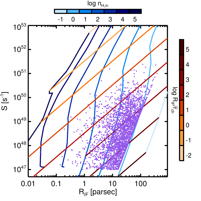
Figure 1.— Radius of the ionization front ($R_{\rm IF}$) versus ionizing luminosity ($S$). Each data point represents a single  H II region at one time step of one of our population synthesis calculations; the line against which points have accumulated on the right side of the plot is the stalling line (see Section 2.2). Colored lines indicate radii and ionizing luminosities of the  H II regions in the RPWW model grid (see Section 2.1); note that only a subset of the models are shown in order to avoid clutter. Blue colors indicate models with constant density $\log n_{\rm H,in}$, and red colors indicate models of constant $\log R_{\rm IF}/\,\tilde{r}_{\rm ch}$, where $\,\tilde{r}_{\rm ch}$ is the characteristic radius at which radiation and gas pressure balance Yeh & Matzner (2012); note that $\,\tilde{r}_{\rm ch}$ is a function of $S$ alone, and does not depend on $R_{\rm IF}$. The values of $\log n_{\rm H,in}$ and $\log R_{\rm IF}/\,\tilde{r}_{\rm ch}$ are as indicated in the color bars.

Figure 1 illustrates the procedure. The Figure shows the ionization front radii ($R_{\rm IF}$) and ionizing luminosities ($S$) of all the  H II regions present at a single time step in one of our population synthesis calculations, overlaid with a grid of models for single  H II regions at an age of 0 Myr. The model grid is characterized by values of density $n_{\rm H,in}$ at the inner edge of the  H II region and by the ratio of the ionization front radius to the characteristic radius $\,\tilde{r}_{\rm ch}$, defined by Yeh & Matzner (2012) as the value of $R_{\rm IF}$ for which gas pressure and unattenuated radiation pressure at the ionization front are equal. This radius is given by

$$\,\tilde{r}_{\rm ch}=\frac{\alpha_{B}L^{2}}{12\pi(2.2k_{B}T_{\rm II}c)^{2}S},$$ (10)

where $k_{B}$ is the Boltzmann constant, $L$ is the bolometric luminosity, $T_{\rm II}=7000$ K is the temperature of the ionized gas and the factor 2.2 is obtained by assuming that helium is singly ionized everywhere. Since $L=\psi S\epsilon_{0}$, the value of $\,\tilde{r}_{\rm ch}$ is simply proportional to $S$. For the simplest case of  H II regions with an age of 0 Myr, we assign each one a luminosity in the [O iii], [N ii], H${\alpha}$ and H${\beta}$ lines by interpolating between the line luminosities of the nearest points in the overlaid model grid. The procedure for older  H II regions is analogous, except that there is an additional interpolation in age. Once we have assigned a luminosity to each  H II region, the total line luminosity of the galaxy is simply the sum over individual  H II regions. Figure 2 shows the final result, where we have used the computed line ratios of both the individual  H II regions from Figure 1 and the integrated galaxy to place them in the BPT diagram.

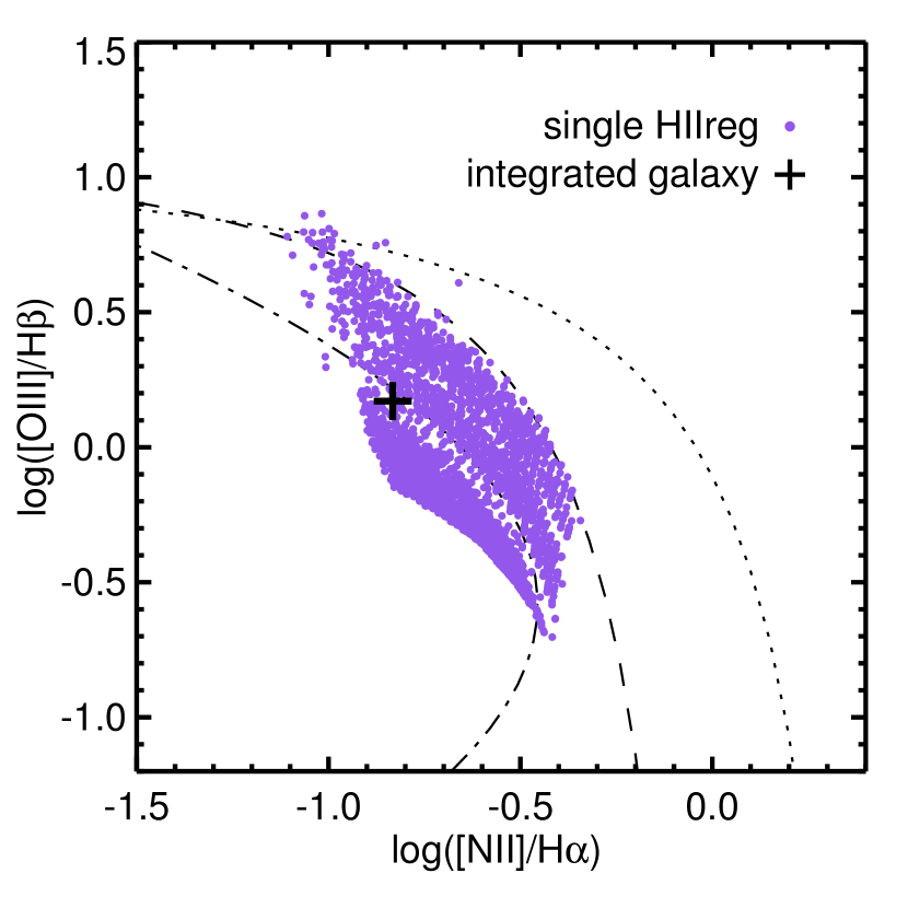
Figure 2.— Result of the interpolation plotted on the BPT plot for one snapshot of a simulated galaxy. The dashed line is the Kauffmann et al. (2003) line, an empirical separation of star forming galaxies and AGN based on the SDSS galaxies. The dotted line is the Kewley et al. (2001) theoretical limit for star forming galaxies. The dot-dashed line is a fit to the star forming galaxies from the SDSS galaxies Brinchmann et al. (2008). Each  H II region is plotted with a dot (as in Figure 1) and the integrated galaxy is shown with the plus sign.

3. Results

Our aim is to investigate how radiation pressure and stellar winds affect galaxies’ emission line ratios. As discussed above, the effects are both internal – changing the density distribution and thus the emission produced within single  H II regions – and external – changing the distribution of  H II region radii and other properties. It is easiest to understand the results if we tackle the internal effects separately first, which we do in Section 3.1. Then in Section 3.2 we consider external effects and how these interact with internal ones. In Section 3.3 we consider how the results depend on the properties of the galaxy as a whole (e.g. star formation rate, ambient pressure).

3.1. Internal effects of radiation pressure and winds

We first examine how our four internal structure models from Table 1 distribute  H II regions in the BPT diagram.

3.1.1 Models with weak winds

We compare the two models with weak winds, RPWW and GPWW, in Figure 3. We show  H II region models with constant $\log n_{\rm H,in}=-1$ to 5 (blue) and with constant $\log R_{\rm IF}/\,\tilde{r}_{\rm ch}$ (red), where $R_{\rm IF}$ is the ionization front radius and $\,\tilde{r}_{\rm ch}$ is the characteristic radius in Krumholz & Matzner (2009) at which radiation and gas pressure balance. The ratio $R_{\rm IF}/\,\tilde{r}_{\rm ch}$ is related to the ionization parameter, as discussed in Paper I. Within each column, we plot three stages of the evolution of the cluster: 0, 2 and 4 Myr (from top to bottom).

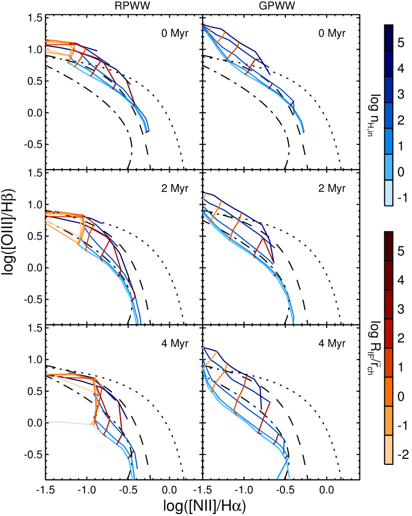
Figure 3.— BPT diagram for the models with weak winds evolving from 0 to 4 Myr (from top to bottom). The left column shows Model RPWW (with radiation pressure) and the right column shows Model GPWW (without radiation pressure). The models are shown with lines of constant $\log n_{\rm H,in}=-1$ to 5 (blue) and constant $\log R_{\rm IF}/\,\tilde{r}_{\rm ch}$ (red), where $R_{\rm IF}$ is the ionization front radius and $\,\tilde{r}_{\rm ch}$ is the characteristic radius in Yeh & Matzner (2012) at which radiation and gas pressure balance.

We confirm some trends that have been seen in the past (Dopita et al., 2000, 2006b; Kewley et al., 2001), such as the decrease of line ratios as the cluster ages and increase of the ionization parameter from bottom right to top left. We explore for the first time a large range of values for the density. We find that the higher the density the stronger the [N ii] and [O iii] emission, up to the point that the gas density exceeds $\sim 10^{4}$ cm^-3. Beyond this, the density in the  H II region exceeds the critical densities of the [N ii] and [O iii] lines ($6.6\times 10^{4}$ cm ^-3 and $6.8\times 10^{5}$ cm^-3, respectively) causing the line intensity to stop increasing. However, before this point is reached, in the highest density models the [O iii] emission is large enough that the [O iii]/H$\beta$ ratio exceeds the upper limit for starburst models described by Kewley et al. (2001) (black dotted line in Figure 3).

We can understand why our models exceed the Kewley et al. (2001) limits as follows. Kewley et al. created a grid of photoionization models with fixed initial density n_H,in = 350 cm^-3 and strong stellar winds (i.e. assuming planar geometry), with a range of metallicities and ionization parameters, and without the effect of radiation pressure. They find that the line ratios in their model never exceed the limit indicated by the black dotted line in Figure 3. Our models exceed this limit because they reach regimes of very high density and very high radiation field that the Kewley et al. models, due to their assumption of a fixed density and planar geometry, are unable to access. The underlying physical processes become clear if we compare our various models. Both models GPWW and RPWW can exceed the Kewley et al. limit, while our strong wind models either do not exceed or barely exceed it (see Section 3.1.2). In model GPWW, the density of the gas near the ionizing source can remain unphysical high even when the luminosity is very high; as a result there is significant emission from high-density, highly-irradiated gas. By contrast, in model RPWW, strong radiation pressure pushes gas away from the ionizing source when the luminosity is high, which in turn reduces the amount of gas that is both dense and highly irradiated. This model still breaks the Kewley et al. limit, but by less than GPWW. When stellar winds are included, on the other hand, the wind pushes the gas away from the source, reducing the radiation flux it experiences. This strongly limits the amount of dense, highly-irradiated gas in both of our strong wind models, and in the Kewley et al. models. We therefore see that the Kewley et al. limit is not a limit imposed by the physics of  H II regions in general; instead, it is driven by Kewley et al.’s assumptions about the structure of  H II regions, and the limitations on density and ionizing luminosity that these assumptions imply.

Comparing the cases with and without radiation pressure, we see that models with radiation pressure often produce less [O iii] emission that those without. This effect arises because  H II regions with radiation pressure and that have $R_{\rm IF}/\,\tilde{r}_{\rm ch}\ll 1$ have most of their gas in a radiation-confined shell that has a steep density gradient. This should be compared to the mostly uniform density produced if one ignores radiation pressure (Draine 2011; Yeh & Matzner 2012; Paper I). The higher density in this shell means that the density in the bulk of the emitting gas can exceed the critical density for a line even when the mean density of the  H II region is below this value. Hence, Model RPWW saturates at a lower value of [O iii]/H$\beta$ than model GPWW.

3.1.2 Models with strong winds

We show the BPT diagram locations of the strong stellar wind models, RPSW and GPSW, in Figure 4. The first thing that is evident from the Figure is that Model RPSW produces line ratios in the BPT diagram far from both the other models and from the locations of observed galaxies. The region of parameter space where the models are not physical within the context of RPSW corresponds to  H II regions with large ionizing luminosities but small radii, and one can understand why Model RPSW avoids this region with a small thought experiment. A value of $\Omega=100$ implies that $P_{\rm IF}V_{\rm IF}/P_{\rm in}V_{\rm in}-1\ll 1$ (see Equation 1), meaning that the shocked wind gas dominates the total energy budget. This in turn requires that $V_{\rm IF}\approx V_{\rm in}$ and $P_{\rm IF}\approx P_{\rm in}$, so that the wind bubble fills almost the entire volume of the  H II region, leaving only a thin shell of photoionized gas, and the gas pressures are nearly identical at the inner and outer edges of this shell. However, if the ionizing luminosity is large enough (specifically if it is large enough so that $R_{\rm IF}<\,\tilde{r}_{\rm ch}$), this is impossible. As $S\rightarrow\infty$ the radiation pressure at the inner edge of the photoionized shell must greatly exceed the gas pressure, and the gas pressure $P_{\rm IF}$ at the outer edge of the  H II region, where all of the radiation has been absorbed, must be equal to the total pressure at the inner edge, which is the sum of the small gas pressure $P_{\rm in}$ and the much larger radiation pressure. It therefore follows that at sufficiently large $S$ one must have $P_{\rm IF}/P_{\rm rad}\gg 1$, giving $\Omega\ll 1$, a point also made by Yeh & Matzner (2012). Thus one cannot simultaneously have arbitrarily large $S$, arbitrarily small $R_{\rm IF}$, and $\Omega\gg 1$. This issue is discussed further in Paper I.

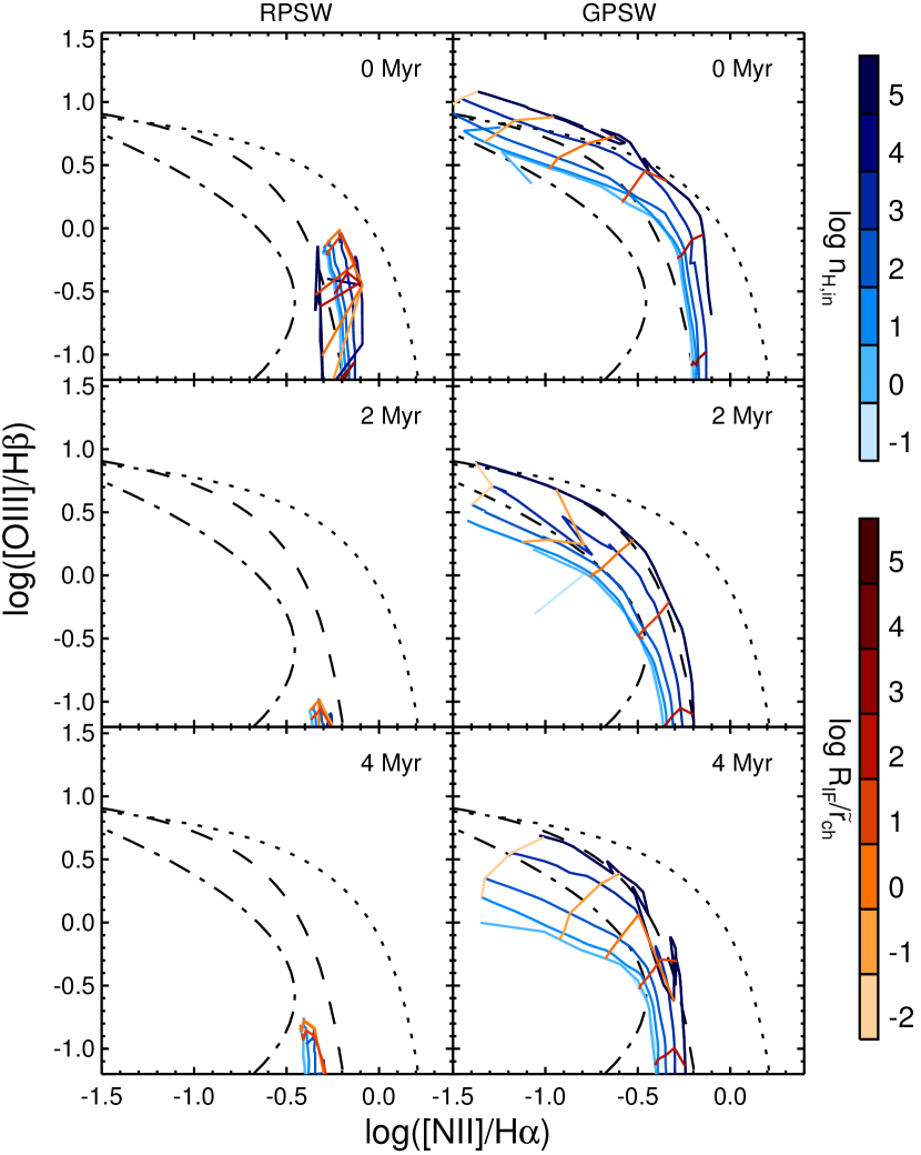
Figure 4.— Same as Figure 3, but for the strong-wind Models GPSW and RPSW.

This problem does not affect Model GPSW, since in this model one ignores radiation pressure. These models thus represent wind-dominated  H II regions, and are qualitatively similar to the models of Dopita et al. (2000) and Kewley et al. (2001). In Paper I, we show a comparison of these models with those of Dopita et al. (2000), and find a good match with their results.

3.2. Dynamical effects of radiation pressure

Having understood the effects of radiation pressure and winds on the internal structure of  H II regions, we are now ready to study their dynamical effects.

3.2.1 Distribution of  H II region radii

Figure 5.— Radius of the ionization front $R_{\rm IF}$ versus ionizing photon luminosity $S$ for all the  H II regions present at one time step in simulated galaxy (dots). We show simulations with two different values of $P_{\rm amb}/k_{B}$ ($10^{4}$ K cm^-3 in the left column, and $10^{6}$ K cm^-3 in the right column), and three different values of $f_{\rm trap}$ (0 in the top row, 2 in the middle row, 50 in the bottom row). Black lines show the location of the stall radii for the simulations, with dashed lines corresponding to stalling when the pressure is gas-dominated, dotted lines to stalling when the pressure is radiation-dominated and full lines when to stalling when both radiation and gas pressure are relevant. The SFR is 1 $M_{\sun}$ yr^-1 in all the simulations shown, so the number of  H II regions present in each panel is approximately the same.

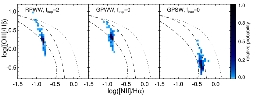
Figure 6.— Synthetic galaxies on the BPT diagram generated with our fiducial parameters and  H II region modeling. Each model is a single time snapshot from our simulations, with the snapshots taken at intervals of 1 Myr. The region shown has been rasterized into pixels of (0.05 dex)². The color in each pixel corresponds to the number of models that fall into that pixel, normalized by the pixel containing the most models. The three cases shown are Model RPWW with $f_{\rm trap}=2$, corresponding to  H II regions with weak winds whose dynamics and internal structure include radiation pressure; Model GPWW with $f_{\rm trap}=0$, corresponding to  H II regions that are classical Strömgren spheres with neither radiation nor wind pressure affecting their internal structure or dynamics; and Model GPSW with $f_{\rm trap}=0$, for which  H II regions are wind-dominated bubbles without radiation pressure.

In the expansion of an  H II region, the radiation pressure term contributes as an additional push towards a faster radial expansion. To study this effect we examine the distribution of  H II region radii produced by our population synthesis code, and how it is influenced by radiation pressure. Figure 5 shows a scatter plot of the radius of the ionization front ($R_{\rm IF}$) versus the ionizing photon luminosity ($S$) for all the  H II regions present at one time step in two of our simulations, one with $P_{\rm amb}/k_{B}=10^{4}$ K cm^-3 (left column) and one with $P_{\rm amb}/k_{B}=10^{6}$ K cm^-3 (right column). We show three cases: $f_{\rm trap}=0$ is a model where radiation pressure does not affect the dynamics at all, $f_{\rm trap}=2$ is our fiducial case, and $f_{\rm trap}=50$ is a model where the radiation pressure is assumed to be strongly trapped within the  H II region, and affects the dynamics much more strongly. The case $f_{\rm trap}=0$ corresponds to  H II regions that follow the classical Spitzer (1978) solution, $f_{\rm trap}=2$ corresponds roughly to the value favored by the radiation-hydrodynamic simulations of Krumholz & Thompson (2012a, b), while $f_{\rm trap}=50$ corresponds to the peak of the values adopted in the subgrid models of Hopkins et al. (2011), where radiation is assumed to build up inside  H II regions and produce large forces. In each panel we also show with full lines the stalling radii, defined as the radii where the internal pressure of the  H II region drops to $P_{\rm amb}$. Each  H II region, when is created, is assigned a value of $S$ and has $R_{\rm IF}=0$. As time passes, the  H II region evolves and moves horizontally in the $R_{\rm IF}$ versus $S$ plane till it reaches this limiting line at the stall radius. Since $P_{\rm rad}/P_{\rm gas}$ decreases as $R_{\rm IF}$ grows at fixed $S$, depending on the value of $S$ and $P_{\rm amb}$, this can happen when $P_{\rm gas}\ll P_{\rm rad}$, when $P_{\rm gas}\gg P_{\rm rad}$, or when $P_{\rm gas}\simeq P_{\rm rad}$. If the  H II region stalls when the gas is dominated by radiation pressure, $P_{\rm amb}\simeq P_{\rm rad}$, and from equation (9) we have $R_{\rm IF}\propto S^{1/2}$; if stalling occurs when an  H II region is dominated by gas pressure, then $P_{\rm amb}\simeq P_{\rm gas}$, and from equation (6) we have $R_{\rm IF}\propto S^{1/3}$. Figure 5 shows also these two dependencies as dotted and dashed lines respectively.

The Figure shows that radiation pressure has two distinct effects on the dynamics. First,  H II regions with radiation pressure expand faster than classical ones, so that models are shifted to increasingly large values of $R_{\rm IF}$ as $f_{\rm trap}$ increases. The shift from $f_{\rm trap}=0$ to 2 is relatively modest, while the gap between $f_{\rm trap}=2$ and 50 is somewhat larger, corresponding to nearly half a dex in radius. The second effect of radiation pressure is to increase the stalling radius. When the ambient pressure is small, this has a relatively small effect, because the stalling radius is large and most  H II regions turn off before reaching it. One the other hand, when the pressure is high, the stalling radius is smaller and most  H II regions stall before their driving stars evolve off the main sequence. In this case most  H II regions are clustered up against the stalling radius, and the increase in stalling radius with $f_{\rm trap}$ has very significant effects.

3.2.2 Distribution of  H II regions in the BPT diagram

We are now ready to use our population synthesis code to determine where simulated galaxies lie in the BPT diagram. We run three classes of models. The first, which we consider the most physically realistic given the observed properties of  H II regions in the local Universe, uses Model RPWW for the internal structures of  H II regions, and uses $f_{\rm trap}=2$ to determine their dynamical evolution. The other two models use $f_{\rm trap}=0$ (i.e. assume that  H II regions expand as classical Spitzer  H II regions), and use Models GPWW and GPSW for the internal structures. The latter choice is not fully consistent, in that with strong wind models we should use a wind-dominated dynamical solution such as that of Castor et al. (1975). We do not do so, however, both because Dopita et al. (2006b) have already explored this case, and because observations now strongly disfavor it.

Figure 6 shows the comparison of the three models on the BPT diagram for our fiducial parameter choices (see Table 2). Each model represents the line ratio produced by summing the line emission over all the  H II regions present in a simulated galaxy at a given snapshot in time, and for each model we show 200 such snapshots, separated by intervals of 1 Myr. The region shown in the plot has been rasterized into pixels of (0.05 dex)². The color in each pixel corresponds to the number of models that fall into that pixel, normalized by the pixel containing the most models. The plot shows several interesting results. Model GPSW, in which  H II regions’ internal structures are wind-dominated, are systematically shifted to lower [O iii]/H$\beta$ and higher [N ii]/h$\alpha$ than the weak wind models. Model RPWW spans a wide range of parameter space, including some snapshots that exceed the Kewley et al. (2001) theoretical limit. These snapshots tend to be immediately after the formation of a very large, bright, association. Model GPWW is covers a smaller range in the plot, and stays below the Kewley et al. (2001) limit.

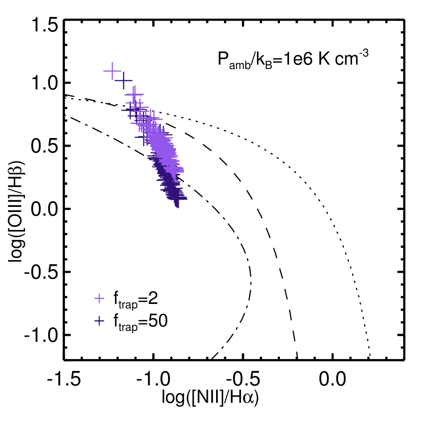
Figure 7.— Comparison of BPT diagrams for two runs with $P_{\rm amb}/k_{B}=10^{6}$ K cm^-3 and $f_{\rm trap}=2$ and 50. Each plus sign represents a single time snapshot from our simulations, with the snapshots taken at intervals of 1 Myr. Both runs use Model RPWW, and are otherwise identical to the runs shown in Figure 6.

We varied a number of the fiducial parameters, and found them to have little effect on the results. Parameters whose influence is negligible include $M_{a,\rm min}$ and $M_{a,\rm max}$, minimum and maximum value of the association mass, $\mathcal{M}$, the Mach number used to set the width of the density distribution, and $k_{\rm\rho}$ the powerlaw index that describes the density distribution into which  H II regions expand. Perhaps surprisingly, the value of $f_{\rm trap}$ also has relatively little effect if we hold the internal models fixed, as illustrated in Figure 7. In other words, if we use Model RPWW to describe the internal structure of  H II regions, the differences in the distributions of  H II region radii visible in Figure 5 as we vary $f_{\rm trap}$ from 0 to 50 do not produce corresponding differences in the locations of the resulting galaxies in the BPT diagram – or at least the differences they produce are mostly within the scatter produced simply by stochastic drawing of association masses and surrounding densities. In Figure 1 we show the grid of models covering over 5 orders of magnitude both in $R_{\rm IF}$ and S. The grid dramatically shrinks in the BPT diagram (Figure 3) causing the small effect of $f_{\rm trap}$ in Figure 7. Thus there does not appear to be an obvious way to use line ratio observations of integrated galaxies to measure the value of the dynamical parameter $f_{\rm trap}$. We stress, however, that $f_{\rm trap}$ includes the influence of wind pressure, and a wind-pressure dominated state can be identified, on the basis of line ratio observations, through its effect on the internal structures of  H II regions. In particular, wind-dominated regions cannot access high values of the ionization parameter and are limited to the lower right of the BPT diagram; see Paper I and Yeh & Matzner (2012) for a thorough discussion.

3.3. Influence of galactic parameters

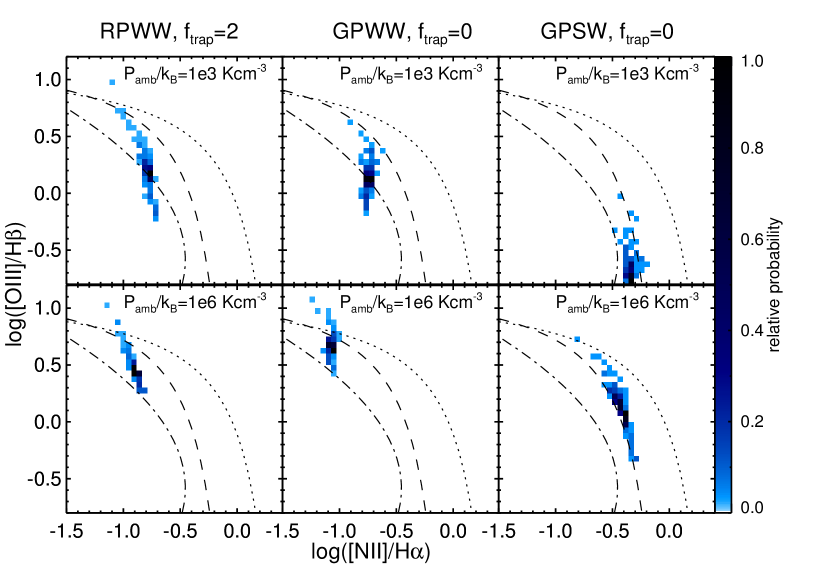
Figure 8.— Simulation results with varying $P_{\rm amb}$. Models RPWW, GPWW, and GPSW are plotted respectively on the left, center and right column for $P_{\rm amb}/k_{B}=10^{3}$ and $10^{6}$ K cm^-3 (top and bottom rows). The region shown has been rasterized into pixels of (0.05 dex)². The color in each pixel corresponds to the number of models that fall into that pixel, normalized by the pixel containing the most models. All other parameters are the same as in the fiducial case.

While there are a number of parameters in our model that make very little difference to the results, the two parameters $P_{\rm amb}$ and SFR that we use to characterize our galaxies do have a measurable influence. Figure 8 shows how the ambient pressure influences the position of simulated galaxies on the BPT diagram. We show our three models computed with $P_{\rm amb}/k_{B}=10^{3}$ and $10^{6}$ K cm^-3 (top and bottom rows). At low ambient pressure, we find a significantly larger spread in the simulated galaxies. This is because for low ambient pressure the stalling radius is large, many  H II regions do not live to reach it, and thus  H II regions span a large range of radii. Exactly where  H II regions fall in the plane of $S$ and $R_{\rm IF}$ is therefore subject to a great deal of stochastic variation. In contrast, as show in Figure 5, increasing the ambient pressure causes all the  H II regions in a galaxy to cluster along the stall radius line. In Figure 8 we can also see that the ambient pressure controls the overall location in the BPT plot, moving all the synthetic galaxies to a higher position in the BPT diagram, and at higher ionization parameter.

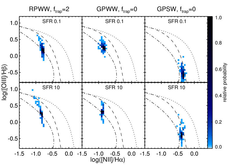
Figure 9.— Same as Figure 8, but here the top and bottom rows correspond to star formation rates of $0.1$ and $10$ $M_{\odot}$ yr^-1. All other parameters are the same as in the fiducial case.

Figure 9 shows the effects of varying the SFR on the location of our synthetic galaxies on the BPT diagram. As the Figure shows, a smaller SFR leads a bigger spread of points in the BPT diagram. This is due to the stochastic nature of star formation at low SFRs, something that can also lead to large variations in absolute line fluxes as well as line ratios (Fumagalli et al., 2011; da Silva et al., 2012; Weisz et al., 2012). If we draw a large mass for the next association to be created, a long time passes until it appears, especially when the SFR is low. During this phase there are no young, bright  H II regions present, and so the galaxy is located in the bottom-right part of the BPT plot. When the association finally forms, the galaxy’s line emission becomes dominated by the resulting bright, young  H II region, which drives it to the top-left part of the BPT diagram. As a result, there is a great deal of variation in the galaxy’s location. When the SFR is high, on the other hand,  H II regions form continuously, causing the population of  H II regions to be more numerous and uniform. We do caution that our mechanism for handling  H II region creation may overestimate the amount of stochasticity found in real galaxies, but that the general sense of the effect will be the same as we have found, even if its magnitude is overestimated. A more realistic formalism for handling the problem of drawing association masses and birth times subject to an overall constraint on the star formation rate is implemented in the SLUG code (da Silva et al., 2012); adding this formalism to our code is left for future work.

4. Comparison to observations

Having understood the physics that drives the location of galaxies in the BPT diagram, we are now in a position to compare our models to observations. Such observations come in two varieties: spatially resolved ones of individual  H II regions or portions of galaxies, and unresolved ones in which the line fluxes from all the  H II regions in a galaxy are summed. Since our code produces collections of stochastically-sampled  H II regions, we can compare to both. For reference and to facilitate comparison, we show in both cases unresolved observations of local galaxies from the SDSS (Brinchmann et al., 2004; Tremonti et al., 2004) along with a fit to this sequence (Brinchmann et al., 2008), the empirically-determined line separating star-forming galaxies from AGN (Kauffmann et al., 2003), and the Kewley et al. (2001) theoretical upper limit to star forming galaxies. The single  H II region sequence and the SDSS star forming galaxy sequence overlap, at least in the upper left part of the BPT diagram, while high redshift galaxies seem to create a different sequence, upward and to the right (Liu et al., 2008; Brinchmann et al., 2008; Hainline et al., 2009; Erb et al., 2010).

Figure 10 shows a collection of observations of single  H II regions and pixel by pixel observations taken from the literature. For the local Universe, our comparison data set consists of single  H II regions from NGC 1365 (Roy & Walsh, 1997), NGC 1313 (Walsh & Roy, 1997), and the Orion region in our own galaxy (Sánchez et al., 2007). We also plot individual pixels in three lensed galaxy at $z\sim 2$ from Jones et al. (2012), which scatter about a locus that passes close to the location of Orion in the BPT diagram. As pointed out by Walter et al. (2009), the SFR surface density of Orion is similar to that of a high redshift object undergoing a burst of star formation.

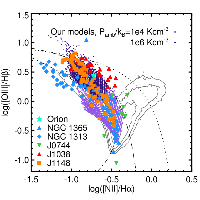
Figure 10.— A comparison between resolved  H II regions and individual  H II regions produced in our simulations in the BPT diagram. We show  H II regions in galaxies at $z=0$ with blue symbols; the galaxies shown are NGC 1365 (Roy & Walsh, 1997) (triangles), NGC 1313 (Walsh & Roy, 1997) (diamonds), and the integrated value for the Orion nebula (Sánchez et al., 2007) (star). We also show single spatial pixels measured with OSIRIS for three lensed galaxies at redshift $z\sim 2.0-2.4$ from (Jones et al., 2012) (green, red, and orange). Contours represent galaxies from the SDSS catalogue (Brinchmann et al., 2004), enclosing respectively, 5, 10, 20, 50, 90 and 99% of all galaxies in which the four emission lines are detected at a greater than 3$\sigma$ significance level. Blue and purple points show the results of our models using fiducial parameters and $P_{\rm amb}/k_{B}=10^{4}$ and $10^{6}$ K cm^-3, respectively. Finally, the dotted line is the theoretical upper limit of Kewley et al. (2001), the dashed line is the empirical AGN - star-forming galaxy separating line (Kauffmann et al., 2003), and the dot-dashed line is the fit to the SDSS sample of Brinchmann et al. (2008).

On top of these data, we overlay the results of our simulations using model RPWW, which we consider most realistic based on observations of nearby  H II regions. The results shown are single snapshots of all the  H II regions produced in two different simulations, one with $P_{\rm amb}/k_{B}=10^{4}$ K cm^-3 one with $10^{6}$ K cm^-3. These two cases should roughly bracket what we expect for Milky Way-like galaxies and for the dense, more strongly star-forming galaxies found at high redshift. The plot shows that our simulations are able to roughly reproduce the locus of observed  H II regions in the BPT diagram for a reasonable range of ambient pressures. We cannot reproduce most of the  H II regions in NGC 1313, because the galaxy has a metallicity lower than solar and our model considers only solar metallicities. Lower metallicity produces a shift of the models towards lower [N ii]/H${\alpha}$ values (Dopita et al., 2000). The pixel by pixel high-$z$ galaxies are best fit by the models with high $P_{\rm amb}$, consistent with observations that these galaxies have high surface and volume densities.

Figure 11 shows the comparison with integrated galaxy measurements; these come from the SDSS for the local Universe, and from a variety of surveys at high-$z$. Many SDSS star forming galaxies lie in the lower part of the star forming sequence due to the presence of a diffuse warm component in the interstellar medium. Brinchmann et al. (2004) point out that a significant amount of the emission line flux in these galaxies comes from the diffuse ionized gas, rather than from  H II regions. The combination of the diffuse ionized gas and the  H II regions typically has a lower effective ionization parameter, and compared to  H II regions alone it shows an enhanced [N ii]/H${\alpha}$ and depressed [O iii]/H${\beta}$ (Mathis, 2000). Therefore, we only expect our models, which do not include the diffuse ionized gas, to reproduce the upper part of the star forming sequence of the SDSS.

In Figure 11 we also overplot the whole-galaxy results produced by our code. As the plot shows, while we are able to reproduce the full spread of individual  H II regions, our simulations of whole galaxies cover a more limited range of BPT than the observations. In particular, we tend to underpredict the observed [N ii]/H$\alpha$ ratios. There are several possible explanations for why we might successfully reproduce individual  H II regions, even in high-$z$ galaxies, but not fully cover the range of integrated galaxy properties. One we have already discussed in the introduction: the offset at high-$z$ may be due to the contribution of a weak AGN, which our models obviously do not include. A second possibility is that the contribution of diffuse ionized gas to the line ratios cannot be neglected even in these high redshift galaxies. Another is that our weighting of the different  H II regions is incorrect because the association mass function is different than the $-2$ powerlaw we have adopted based on local observations, or because of biases introduced by dust extinction, despite the extinction-independent nature of the BPT line ratios (see Yeh & Matzner 2012). A fourth possibility is that our lognormal distribution of densities provides a poor fit to the true range of densities into which  H II regions expand in high-$z$ galaxies, so that the amount of time individual  H II regions spend in the upper left versus the lower right parts of the BPT diagram is off in our models.

As a last possibility, we recognize that the ability of our models for individual  H II regions to reproduce the observations of Orion very well (Figure 10) may be partly a matter of good luck. Our models are not designed to mimic the champagne flow phase of young ($<10^{5}$ yr), compact  H II regions. In particular, we assume a state of quasi-static force balance which holds only approximately in accelerating flows; see Yeh & Matzner (2012) § 3.4 on this point. Indeed, Orion does not resemble the typical  H II region - e.g., a few million years old and at the stalling radius - in our galaxy simulations. It is possible that the different distribution of high-$z$ galaxies in the BPT plot as compared to local SDSS galaxies is due to the higher pressure environment in the former, which keeps the  H II regions longer in a champagne flow-like phase. Future studies might assess our models’ accuracy in the champagne phase, extend their range of validity, and quantify the importance of this dynamical detail for high-$z$ galaxies.

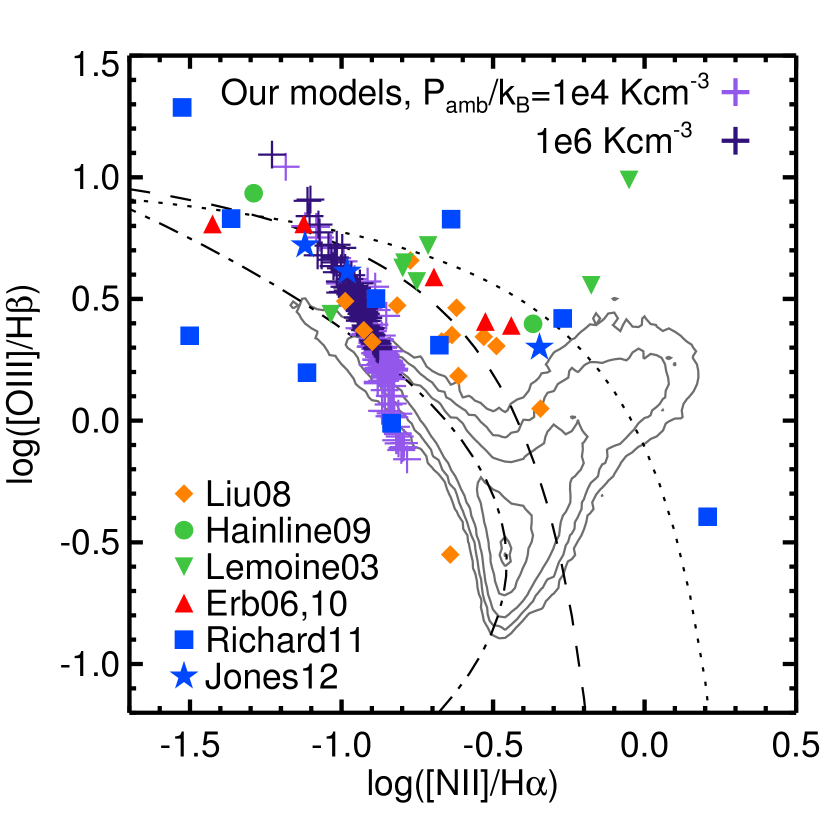
Figure 11.— A comparison between observed unresolved galaxies and simulated produced by our code in the BPT diagram. Contours and lines are the same as in Figure 10. Diamonds show galaxies at $z\sim 1-1.4$ taken from the DEEP2 survey Shapley et al. (2005); Liu et al. (2008); triangles show galaxies at $z\sim 2$ taken from Erb et al. (2006, 2010); lensed galaxies at a variety of redshifts and samples are indicated by inverted triangles (Lemoine-Busserolle et al., 2003), circles (Hainline et al., 2009), squares (Richard et al., 2011), and stars (Jones et al., 2012). Blue and purple plus signs show the results for integrated galaxies in of our models using fiducial parameters, Model RPWW, and ambient pressures of $P_{\rm amb}/k_{B}=10^{4}$ and $10^{6}$ K cm^-3. Each point represents a single time snapshot taken at 1 Myr intervals from a simulation that evolves for 200 Myr.

5. Discussion and Conclusions

Motivated by recent observations suggesting that  H II regions are shaped much less than expected by the pressure of shocked stellar wind gas, and much more by direct radiation pressure (Harper-Clark & Murray, 2009; Lopez et al., 2011; Yeh & Matzner, 2012), we revisit the problem of determining the line flux emitted by a population of  H II regions. We adopt as our default a model of  H II regions where the pressure of winds is subdominant, and radiation pressure is not neglected, and we compare this result to traditional models with strong winds and weak radiation pressure. In Paper I we discuss how we generate grids of static, single  H II regions, with a wide range of sizes and ionizing luminosities, with varying strengths of winds and radiation pressure. In this paper we construct dynamical expansion models for these  H II regions, and explore how changing the strength of winds and radiation pressure affects their line ratios in the BPT diagram. We find that radiation pressure has two important effects. First, $P_{\rm rad}$ changes the internal structure of the  H II region, creating a density gradient towards the outer shell. This affects the expected line emission, allowing the  H II regions to exceed the upper limit form starburst models set by Kewley et al. (2001). Second, radiation pressure provides an extra boost to the expansion, leading to larger radii at earlier times.

We embed these models in a population synthesis code that generates galactic collections of stochastically-generated  H II regions expanding into a turbulent medium. The code follows  H II regions as they are born, evolve, stall and die. Using this code we predict the integrated line emission of galaxies as a function of several galactic properties. We find that the two most important ones in controlling where galaxies appear in the BPT diagram are the ambient pressure, which shifts galaxies up and to the left as it increases, and the star formation rate, which affects the amount of stochastic scatter in a galaxy’s line ratios.

We compare with observations in two distinct ways. First, we select single  H II regions observed in the local universe and pixel by pixel observations of $z\sim 2$ galaxies, and we compare these to the distributions of individual  H II regions produced in our model. We show that our model produces good agreement with the observations for reasonable ranges of SFR and ambient pressure. The high redshift pixel data are best reproduced by  H II regions evolving in a high pressure medium and with high SFR, which we interpret as a sign of intense star formation in a dense interstellar medium, consistent with the observed properties of high-$z$ galaxies (e.g. Elmegreen et al., 2009; Genzel et al., 2011).

Second, we compare integrated galaxies from the SDSS catalogue and the high redshift universe to our synthetic galaxies. We find that, while we are able to reproduce the spread of individual  H II regions, our models for integrated galaxies cluster too tightly compared to the observed range of line ratios in real galaxies, particularly at high-$z$. This might be due to a number of factors. One possibility is that the lognormal distribution of the ambient density we have adopted is a poor description of the density distribution in high-$z$ galactic disks. Another possibility is that winds might be important at high redshift or that the presence of the diffuse ionized medium is not negligible. A third possibility is that a higher pressure environment in high-z galaxies keeps the  H II regions longer in a champagne flow-like phase. One last possibility is that $z\sim 2$ star forming galaxies may contain an AGN that partially contributes to the line emission. We leave these possibilities as a subject for future work.

References

- Baldwin et al. (1981) Baldwin, J. A., Phillips, M. M., & Terlevich, R. 1981, PASP, 93, 5
- Brinchmann et al. (2004) Brinchmann, J., Charlot, S., White, S. D. M., et al. 2004, MNRAS, 351, 1151
- Brinchmann et al. (2008) Brinchmann, J., Pettini, M., & Charlot, S. 2008, MNRAS, 385, 769
- Castor et al. (1975) Castor, J., McCray, R., & Weaver, R. 1975, ApJ, 200, L107
- da Silva et al. (2012) da Silva, R. L., Fumagalli, M., & Krumholz, M. 2012, ApJ, 745, 145
- Dopita et al. (2000) Dopita, M. A., Kewley, L. J., Heisler, C. A., & Sutherland, R. S. 2000, ApJ, 542, 224
- Dopita et al. (2005) Dopita, M. A., Groves, B. A., Fischera, J., et al. 2005, ApJ, 619, 755
- Dopita et al. (2006a) Dopita, M. A., Fischera, J., Sutherland, R. S., et al. 2006a, ApJ, 647, 244
- Dopita et al. (2006b) —. 2006b, ApJS, 167, 177
- Draine (2011) Draine, B. T. 2011, ApJ, 732, 100
- Elmegreen et al. (2009) Elmegreen, D. M., Elmegreen, B. G., Marcus, M. T., et al. 2009, ApJ, 701, 306
- Erb et al. (2010) Erb, D. K., Pettini, M., Shapley, A. E., et al. 2010, ApJ, 719, 1168
- Erb et al. (2006) Erb, D. K., Shapley, A. E., Pettini, M., et al. 2006, ApJ, 644, 813
- Fall et al. (2010) Fall, S. M., Krumholz, M. R., & Matzner, C. D. 2010, ApJ, 710, L142
- Ferland et al. (1998) Ferland, G. J., Korista, K. T., Verner, D. A., et al. 1998, PASP, 110, 761
- Fumagalli et al. (2011) Fumagalli, M., da Silva, R. L., & Krumholz, M. R. 2011, ApJ, 741, L26
- Genzel et al. (2011) Genzel, R., Newman, S., Jones, T., et al. 2011, ApJ, 733, 101
- Goldbaum et al. (2011) Goldbaum, N. J., Krumholz, M. R., Matzner, C. D., & McKee, C. F. 2011, ApJ, 738, 101
- Groves et al. (2008) Groves, B., Dopita, M. A., Sutherland, R. S., et al. 2008, ApJS, 176, 438
- Hainline et al. (2009) Hainline, K. N., Shapley, A. E., Kornei, K. A., et al. 2009, ApJ, 701, 52
- Harper-Clark & Murray (2009) Harper-Clark, E., & Murray, N. 2009, ApJ, 693, 1696
- Hopkins et al. (2011) Hopkins, P. F., Quataert, E., & Murray, N. 2011, MNRAS, 1513, in press, arXiv:1101.4940
- Jones et al. (2012) Jones, T., Ellis, R. S., Richard, J., & Jullo, E. 2012, ArXiv e-prints
- Kauffmann et al. (2003) Kauffmann, G., Heckman, T. M., Tremonti, C., et al. 2003, MNRAS, 346, 1055
- Kewley et al. (2001) Kewley, L. J., Dopita, M. A., Sutherland, R. S., Heisler, C. A., & Trevena, J. 2001, ApJ, 556, 121
- Kroupa (2001) Kroupa, P. 2001, MNRAS, 322, 231
- Krumholz & Matzner (2009) Krumholz, M. R., & Matzner, C. D. 2009, ApJ, 703, 1352
- Krumholz et al. (2006) Krumholz, M. R., Matzner, C. D., & McKee, C. F. 2006, ApJ, 653, 361
- Krumholz & Thompson (2007) Krumholz, M. R., & Thompson, T. A. 2007, ApJ, 669, 289
- Krumholz & Thompson (2012a) —. 2012a, ApJ, submitted, arXiv:1203.2926
- Krumholz & Thompson (2012b) —. 2012b, ApJ, in preparation
- Leitherer et al. (1999) Leitherer, C., Schaerer, D., Goldader, J. D., et al. 1999, ApJS, 123, 3
- Lemoine-Busserolle et al. (2003) Lemoine-Busserolle, M., Contini, T., Pelló, R., et al. 2003, A&A, 397, 839
- Liu et al. (2008) Liu, X., Shapley, A. E., Coil, A. L., Brinchmann, J., & Ma, C.-P. 2008, ApJ, 678, 758
- Lopez et al. (2011) Lopez, L. A., Krumholz, M. R., Bolatto, A. D., Prochaska, J. X., & Ramirez-Ruiz, E. 2011, ApJ, 731, 91
- Mathis (2000) Mathis, J. S. 2000, ApJ, 544, 347
- Murray et al. (2010) Murray, N., Quataert, E., & Thompson, T. A. 2010, ApJ, 709, 191
- Murray & Rahman (2010) Murray, N., & Rahman, M. 2010, ApJ, 709, 424
- Padoan & Nordlund (2002) Padoan, P., & Nordlund, Å. 2002, ApJ, 576, 870
- Parravano et al. (2003) Parravano, A., Hollenbach, D. J., & McKee, C. F. 2003, ApJ, 584, 797
- Pellegrini et al. (2011) Pellegrini, E. W., Baldwin, J. A., & Ferland, G. J. 2011, ApJ, 738, 34
- Richard et al. (2011) Richard, J., Jones, T., Ellis, R., et al. 2011, MNRAS, 413, 643
- Roy & Walsh (1997) Roy, J.-R., & Walsh, J. R. 1997, MNRAS, 288, 715
- Sánchez et al. (2007) Sánchez, S. F., Cardiel, N., Verheijen, M. A. W., et al. 2007, A&A, 465, 207
- Shapley et al. (2005) Shapley, A. E., Coil, A. L., Ma, C.-P., & Bundy, K. 2005, ApJ, 635, 1006
- Spitzer (1978) Spitzer, L. 1978, Physical processes in the interstellar medium (Wiley-Interscience)
- Sutherland & Dopita (1993) Sutherland, R. S., & Dopita, M. A. 1993, ApJS, 88, 253
- Townsley et al. (2003) Townsley, L. K., Feigelson, E. D., Montmerle, T., et al. 2003, ApJ, 593, 874
- Tremonti et al. (2004) Tremonti, C. A., Heckman, T. M., Kauffmann, G., et al. 2004, ApJ, 613, 898
- Trump et al. (2011) Trump, J. R., Weiner, B. J., Scarlata, C., et al. 2011, ApJ, 743, 144
- Walsh & Roy (1997) Walsh, J. R., & Roy, J.-R. 1997, MNRAS, 288, 726
- Walter et al. (2009) Walter, F., Riechers, D., Cox, P., et al. 2009, Nature, 457, 699
- Weaver et al. (1977) Weaver, R., McCray, R., Castor, J., Shapiro, P., & Moore, R. 1977, ApJ, 218, 377
- Weisz et al. (2012) Weisz, D. R., Johnson, B. D., Johnson, L. C., et al. 2012, ApJ, 744, 44
- Williams & McKee (1997) Williams, J. P., & McKee, C. F. 1997, ApJ, 476, 166
- Wright et al. (2010) Wright, S. A., Larkin, J. E., Graham, J. R., & Ma, C.-P. 2010, ApJ, 711, 1291
- Yeh & Matzner (2012) Yeh, S. C. C., & Matzner, C. D. 2012, ArXiv e-prints
- Yeh et al. (2012) Yeh, S. C. C., Verdolini, S., Krumholz, M. R., Matzner, C. D., & Tielens, A. G. G. M. 2012, ApJ, submitted