Variational Semi-blind Sparse Deconvolution with Orthogonal Kernel Bases and its Application to MRFM

Abstract

We present a variational Bayesian method of joint image reconstruction and point spread function (PSF) estimation when the PSF of the imaging device is only partially known. To solve this semi-blind deconvolution problem, prior distributions are specified for the PSF and the 3D image. Joint image reconstruction and PSF estimation is then performed within a Bayesian framework, using a variational algorithm to estimate the posterior distribution. The image prior distribution imposes an explicit atomic measure that corresponds to image sparsity. Importantly, the proposed Bayesian deconvolution algorithm does not require hand tuning. Simulation results clearly demonstrate that the semi-blind deconvolution algorithm compares favorably with previous Markov chain Monte Carlo (MCMC) version of myopic sparse reconstruction. It significantly outperforms mismatched non-blind algorithms that rely on the assumption of the perfect knowledge of the PSF. The algorithm is illustrated on real data from magnetic resonance force microscopy (MRFM).

1 Introduction

The standard and popular image deconvolution techniques generally assume that the space-invariant instrument response, i.e., the point spread function (PSF), is perfectly known. However, in many practical situations, the true PSF is either unknown or, at best, partially known. For example, in an optical system a perfectly known PSF does not exist because of light diffraction, apparatus/lense aberration, out-of-focus, or image motion [1, 2]. Such imperfections are common in general imaging systems including MRFM, where there exist additional model PSF errors in the sensitive magnetic resonance condition [3]. In such circumstances, the PSF required in the reconstruction process is mismatched with the true PSF. The quality of standard image reconstruction techniques may suffer from this disparity. To deal with this mismatch, deconvolution methods have been proposed to estimate the unknown image and the PSF jointly. When prior knowledge of the PSF is available, these methods are usually referred to as semi-blind deconvolution [4, 5] or myopic deconvolution [6, 7, 8].

In this paper, we formulate the semi-blind deconvolution task as an estimation problem in a Bayesian setting. Bayesian estimation has the great advantage of offering a flexible framework to solve complex model-based problems. Prior information available on the parameters to be estimated can be efficiently included within the model, leading to an implicit regularization of our ill-posed problem. In addition, the Bayes framework produces posterior estimates of uncertainty, via posterior variance and posterior confidence intervals. Extending our previous work, we propose a variational estimator for the parameters as contrasted to the Monte Carlo approach in [9]. This extension is non-trivial. Our variational Bayes algorithm iterates on a hidden variable domain associated with the mixture coefficients. This algorithm is faster, more scalable for equivalent image reconstruction qualities in [9].

Like in [9], the PSF uncertainty is modeled as the deviation of the a priori known PSF from the true PSF. Applying an eigendecomposition to the PSF covariance, the deviation is represented as a linear combination of orthogonal PSF bases with unknown coefficients that need to be estimated. Furthermore, we assume the desired image is sparse, corresponding to the natural sparsity of the molecular image. The image prior is a weighted sum of a sparsity inducing part and a continuous distribution; a positive truncated Laplacian and atom at zero (LAZE) prior [10]. Similar priors have been applied to estimating mixtures of densities [11, 12, 13] and sparse, nonnegative hyperspectral unmixing [14]. Here we introduce a hidden label variable for the contribution of the discrete mass (empty pixel) and a continuous density function (non-empty pixel). Similar to our ‘hybrid’ mixture model, inhomogeneous gamma-Gaussian mixture models have been proposed in [15].

Bayesian inference of parameters from the posterior distribution generally requires challenging computations, such as functional optimization and numerical integration. One widely advocated strategy relies on approximations to the minimum mean square error (MMSE) or maximum a posteriori (MAP) estimators using samples drawn from the posterior distribution. Generation of these samples can be accomplished using Markov chain Monte Carlo methods (MCMC) [16]. MCMC has been successfully adopted in numerous imaging problems such as image segmentation, denoising, and deblurring [17, 16]. Recently, to solve blind deconvolution, two promising semi-blind MCMC methods have been suggested [9, 18]. However, these sampling methods have the disadvantage that convergence may be slow.

An alternative to Monte Carlo integration is a variational approximation to the posterior distribution, and this approach is adopted in this paper. These approximations have been extensively exploited to conduct inference in graphical models [19]. If properly designed, they can produce an analytical posterior distribution from which Bayesian estimators can be efficiently computed. Compared to MCMC, variational methods are of lower computational complexity, since they avoid stochastic simulation. However, variational Bayes (VB) approaches have intrinsic limits; the convergence to the true distribution is not guaranteed, even though the posterior distribution will be asymptotically normal with mean equal to the maximum likelihood estimator under suitable conditions [20]. In addition, variational Bayes approximations can be easily implemented for only a limited number of statistical models. For example, this method is difficult to apply when latent variables have distributions that do not belong to the exponential family (e.g. a discrete distribution [9]). For mixture distributions, variational estimators in Gaussian mixtures and in exponential family converge locally to maximum likelihood estimator [21, 22]. The theoretical convergence properties for sparse mixture models, such as our proposed model, are as yet unknown. This has not hindered the application of VB to sparse models to problems in our sparse image mixture model. Another possible intrinsic limit of the variational Bayes approach, particularly in (semi)-blind deconvolution, is that the posterior covariance structure cannot be effectively estimated nor recovered, unless the true joint distributions have independent individual distributions. This is primarily because VB algorithms are based on minimizing the KL-divergence between the true distribution and the VB approximating distribution, which is assumed to be factorized with respect to the individual parameters.

However, despite these limits, VB approaches have been widely applied with success to many different engineering problems [23, 24, 25, 26]. A principal contribution of this paper is the development and implementation of a VB algorithm for mixture distributions in a hierarchical Bayesian model. Similarly, the framework permits a Gaussian prior [27] or a Student’s-t prior [28] for the PSF. We present comparisons of our variational solution to other blind deconvolution methods. These include the total variation (TV) prior for the PSF [29] and natural sharp edge priors for images with PSF regularization [30]. We also compare to basis kernels [28], the mixture model algorithm of Fergus et al. [31], and the related method of Shan et al. [32] under a motion blur model.

To implement variational Bayesian inference, prior distributions and the instrument-dependent likelihood function are specified. Then the posterior distributions are estimated by minimizing the Kullback-Leibler (KL) distance between the model and the empirical distribution. Simulations conducted on synthetic images show that the resulting myopic deconvolution algorithm outperforms previous mismatched non-blind algorithms and competes with the previous MCMC-based semi-blind method [9] with lower computational complexity.

We illustrate the proposed method on real data from magnetic resonance force microscopy (MRFM) experiments. MRFM is an emerging molecular imaging modality that has the potential for achieving $3$D atomic scale resolution [33, 34, 35]. Recently, MRFM has successfully demonstrated imaging [36, 37] of a tobacco mosaic virus [38]. The $3$D image reconstruction problem for MRFM experiments was investigated with Wiener filters [39, 40, 37], iterative least square reconstruction approaches [41, 38, 42], and recently the Bayesian estimation framework [10, 43, 8, 9]. The drawback of these approaches is that they require prior knowledge on the PSF. However, in many practical situations of MRFM imaging, the exact PSF, i.e., the response of the MRFM tip, is only partially known [3]. The proposed semi-blind reconstruction method accounts for this partial knowledge.

The rest of this paper is organized as follows. Section 2 formulates the imaging deconvolution problem in a hierarchical Bayesian framework. Section 3 covers the variational methodology and our proposed solutions. Section 4 reports simulation results and an application to the real MRFM data. Section 5 discusses our findings and concludes.

2 Formulation

2.1 Image Model

As in [9, 43], the image model is defined as:

$$\mathbf{y}=\mathbf{H}{\mathbf{x}}+\mathbf{n}=T\left(\boldsymbol{\kappa},{\mathbf{x}}\right)+\mathbf{n},$$ (1)

where $\mathbf{y}$ is a $P\times 1$ vectorized measurement, ${\mathbf{x}}=[x_{1},\ldots,x_{N}]^{T}\succeq 0$ is an $N\times 1$ vectorized sparse image to be recovered, $T\left(\boldsymbol{\kappa},\cdot\right)$ is a convolution operator with the PSF $\boldsymbol{\kappa}$, $\mathbf{H}=[{\mathbf{h}}_{1},\ldots,{\mathbf{h}}_{N}]$ is an equivalent system matrix, and $\mathbf{n}$ is the measurement noise vector. In this work, the noise vector $\mathbf{n}$ is assumed to be Gaussian, $\mathbf{n}\sim{\mathcal{N}}\left(\boldsymbol{0},{\sigma^{2}}\textbf{I}_{P}\right)$. The PSF $\boldsymbol{\kappa}$ is assumed to be unknown but a nominal PSF estimate $\boldsymbol{\kappa}_{0}$ is available. The semi-blind deconvolution problem addressed in this paper consists of the joint estimation of ${\mathbf{x}}$ and $\boldsymbol{\kappa}$ from the noisy measurements $\mathbf{y}$ and nominal PSF $\boldsymbol{\kappa}_{0}$.

2.2 PSF Basis Expansion

The nominal PSF $\boldsymbol{\kappa}_{0}$ is assumed to be generated with known parameters (gathered in the vector $\boldsymbol{\zeta_{0}}$) tuned during imaging experiments. However, due to model mismatch and experimental errors, the true PSF $\boldsymbol{\kappa}$ may deviate from the nominal PSF $\boldsymbol{\kappa}_{0}$. If the generation model for PSFs is complex, direct estimation of a parameter deviation, $\Delta\boldsymbol{\zeta}=\boldsymbol{\zeta_{true}}-\boldsymbol{\zeta_{0}}$, is difficult.

We model the PSF $\boldsymbol{\kappa}$ (resp. $\{{\mathbf{H}}\}$) as a perturbation about a nominal PSF $\boldsymbol{\kappa}_{0}$ (resp. $\{{\mathbf{H}}^{0}\}$) with $K$ basis vectors $\boldsymbol{\kappa}_{k}$, $k=1,\ldots,K$, that span a subspace representing possible perturbations $\Delta\boldsymbol{\kappa}$. We empirically determined this basis using the following PSF variational eigendecomposition approach. A number of PSFs $\tilde{\boldsymbol{\kappa}}$ are generated following the PSF generation model with parameters $\boldsymbol{\zeta}$ randomly drawn according to Gaussian distribution centered at the nominal values $\boldsymbol{\zeta_{0}}$. Then a standard principal component analysis (PCA) of the residuals $\left\{\tilde{\boldsymbol{\kappa}}_{j}-\boldsymbol{\kappa}_{0}\right\}_{j=1,\ldots}$ is used to identify $K$ principal axes that are associated with the basis vectors $\boldsymbol{\kappa}_{k}$. The necessary number of basis vectors, $K$, is determined empirically by detecting a knee at the scree plot. The first few eigenfunctions, corresponding to the first few largest eigenvalues, explain major portion of the observed perturbations. If there is no PSF generation model, then we can decompose the support region of the true (suspected) PSF to produce an orthonormal basis. The necessary number of the bases is again chosen to explain most support areas that have major portion/energy of the desired PSF. This approach is presented in our experiment with Gaussian PSFs.

We use a basis expansion to present $\boldsymbol{\kappa}({\mathbf{c}})$ as the following linear approximation to $\boldsymbol{\kappa}$,

$$\boldsymbol{\kappa}({\mathbf{c}})=\boldsymbol{\kappa}_{0}+\sum_{i=1}^{K}c_{i}\boldsymbol{\kappa}_{i},$$ (2)

where the $\{c_{i}\}$ determine the PSF relative to this bases. With this parameterization, the objective of semi-blind deconvolution is to estimate the unknown image, ${\mathbf{x}}$, and the linear expansion coefficients ${\mathbf{c}}=[c_{1},\ldots,c_{K}]^{T}$.

2.3 Determination of Priors

The priors on the PSF, the image, and the noise are constructed as latent variables in a hierarchical Bayesian model.

2.3.1 Likelihood function

Under the hypothesis that the noise in (1) is white Gaussian, the likelihood function takes the form

$$p\left(\mathbf{y}|{\mathbf{x}},{\mathbf{c}},{\sigma^{2}}\right)= \left(\frac{1}{2\pi\sigma^{2}}\right)^{\frac{P}{2}}\times$$

$$\exp\left(-\frac{\left\|\mathbf{y}-T\left(\boldsymbol{\kappa}\left({\mathbf{c}}\right),{\mathbf{x}}\right)\right\|^{2}}{2{\sigma^{2}}}\right),$$ (3)

where $\left\|\cdot\right\|$ denotes the $\ell_{2}$ norm $\left\|{\mathbf{x}}\right\|^{2}={\mathbf{x}}^{T}{\mathbf{x}}$.

2.3.2 Image and label priors

To induce sparsity and positivity of the image, we use an image prior consisting of “a mixture of a point mass at zero and a single-sided exponential distribution” [10, 43, 9]. This prior is a convex combination of an atom at zero and an exponential distribution:

$$p(x_{i}|a,w)=(1-w)\delta(x_{i})+wg(x_{i}|a).$$ (4)

In (4), $\delta(\cdot)$ is the Dirac delta function, $w=\mathrm{P}\left(x_{i}\neq 0\right)$ is the prior probability of a non-zero pixel and $g(x_{i}|a)=\frac{1}{a}\exp\left(-\frac{x_{i}}{a}\right)\boldsymbol{1}_{\mathbb{R}^{*}_{+}}(x_{i})$ is a single-sided exponential distribution where $\mathbb{R}^{*}_{+}$ is a set of positive real numbers and $\boldsymbol{1}_{\mathbb{E}}(\cdot)$ denotes the indicator function on the set $\mathbb{E}$:

$$\boldsymbol{1}_{\mathbb{E}}(x)=\left\{\begin{array}[]{ll}1,&\hbox{if $x\in\mathbb{E}$;}\\ 0,&\hbox{otherwise.}\end{array}\right.$$ (5)

A distinctive property of the image prior (4) is that it can be expressed as a latent variable model

$$p(x_{i}|a,z_{i})=(1-z_{i})\delta(x_{i})+z_{i}g(x_{i}|a),$$ (6)

where the binary variables $\{z_{i}\}_{1}^{N}$ are independent and identically distributed and indicate if the pixel $x_{i}$ is active

$$z_{i}=\left\{\begin{array}[]{ll}1,&\hbox{if $x_{i}\neq 0$;}\\ 0,&\hbox{otherwise.}\end{array}\right.$$ (7)

and have the Bernoulli probabilities: $z_{i}\sim Ber(w)$.

The prior distribution of pixel value $x_{i}$ in (4) can be rewritten conditionally upon latent variable $z_{i}$

$$p\left(x_{i}|z_{i}=0\right) =\delta\left(x_{i}\right),$$

$$p\left(x_{i}|a,z_{i}=1\right) =g\left(x_{i}|a\right),$$

which can be summarized in the following factorized form

$$p(x_{i}|a,z_{i})=\delta(x_{i})^{1-z_{i}}g(x_{i}|a)^{z_{i}}.$$ (8)

By assuming each component $x_{i}$ to be conditionally independent given $z_{i}$ and $a$, the following conditional prior distribution is obtained for $\mathbf{x}$:

$$p(\mathbf{x}|a,\mathbf{z})=\prod_{i=1}^{N}\left[\delta(x_{i})^{1-z_{i}}g(x_{i}|a)^{z_{i}}\right]$$ (9)

where $\mathbf{z}=\left[z_{1},\ldots,z_{N}\right]$.

This factorized form will turn out to be crucial for simplifying the variational Bayes reconstruction algorithm in Section 3.

2.3.3 PSF parameter prior

We assume that the PSF parameters $c_{1},\ldots,c_{K}$ are independent and $c_{k}$ is uniformly distributed over intervals

$${\mathcal{S}}_{k}=\left[-\Delta c_{k},\Delta c_{k}\right].$$ (10)

These intervals are specified a priori and are associated with error tolerances of the imaging instrument. The joint prior distribution of ${\mathbf{c}}=\left[c_{1},\ldots,c_{K}\right]^{T}$ is therefore:

$$p\left({\mathbf{c}}\right)=\prod_{k=1}^{K}\frac{1}{2\Delta c_{k}}\textbf{1}_{{\mathcal{S}}_{k}}\left(c_{k}\right).$$ (11)

2.3.4 Noise variance prior

A conjugate inverse-Gamma distribution with parameters $\varsigma_{0}$ and $\varsigma_{1}$ is assumed as the prior distribution for the noise variance (See A.1 for the details of this distribution):

$${\sigma^{2}}|\varsigma_{0},\varsigma_{1}\sim{\mathcal{I}}{\mathcal{G}}\left(\varsigma_{0},\varsigma_{1}\right).$$ (12)

The parameters $\varsigma_{0}$ and $\varsigma_{1}$ will be fixed to a number small enough to obtain a vague hyperprior, unless we have good prior knowledge.

2.4 Hyperparameter Priors

As reported in [10, 43], the values of the hyperparameters $\left\{a,w\right\}$ greatly impact the quality of the deconvolution. Following the approach in [9], we propose to include them within the Bayesian model, leading to a second level of hierarchy in the Bayesian paradigm. This hierarchical Bayesian model requires the definition of prior distributions for these hyperparameters, also referred to as hyperpriors which are defined below.

2.4.1 Hyperparameter $a$

A conjugate inverse-Gamma distribution is assumed for the Laplacian scale parameter $a$:

$$a|\boldsymbol{\alpha}\sim{\mathcal{I}}{\mathcal{G}}\left(\alpha_{0},\alpha_{1}\right),$$ (13)

with $\boldsymbol{\alpha}=\left[\alpha_{0},\alpha_{1}\right]^{T}$. The parameters $\alpha_{0}$ and $\alpha_{1}$ will be fixed to a number small enough to obtain a vague hyperprior, unless we have good prior knowledge.

2.4.2 Hyperparameter $w$

We assume a Beta random variable with parameters $(\beta_{0},\beta_{1})$, which are iteratively updated in accordance with data fidelity. The parameter values will reflect the degree of prior knowledge and we set $\beta_{0}=\beta_{1}=1$ to obtain a non-informative prior. (See A.2 for the details of this distribution)

$$w\sim{\mathcal{B}}(\beta_{0},\beta_{1}).$$ (14)

2.5 Posterior Distribution

The conditional relationships between variables is illustrated in Fig. 1. The resulting posterior of hidden variables given the observation is

$$p({\mathbf{x}},a,{\mathbf{z}},w,{\mathbf{c}},\sigma^{2}|{\mathbf{y}})\propto p({\mathbf{y}}|{\mathbf{x}},{\mathbf{c}},\sigma^{2})\\ \times p({\mathbf{x}}|a,{\mathbf{z}})p({\mathbf{z}}|w)p(w)p(a)p({\mathbf{c}})p(\sigma^{2}).$$ (15)

Since it is too complex to derive exact Bayesian estimators from this posterior, a variational approximation of this distribution is proposed in the next section.

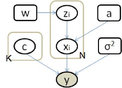
Figure 1: Conditional relationships between variables. A node at an arrow tail conditions the node at the arrow head.

3 Variational Approximation

3.1 Basics of Variational Inference

In this section, we show how to approximate the posterior densities within a variational Bayes framework. Denote by ${\mathbf{U}}$ the set of all hidden parameter variables including the image variable ${\mathbf{x}}$ in the model, denoted by ${\mathcal{M}}$. The hierarchical model implies the Markov representation $p({\mathbf{y}},{\mathbf{U}}|{\mathcal{M}})=p({\mathbf{y}}|{\mathbf{U}},{\mathcal{M}})p({\mathbf{U}}|{\mathcal{M}})$. Our objective is to compute the posterior $p({\mathbf{x}}|{\mathbf{y}},{\mathcal{M}})=\int p({\mathbf{y}}|{\mathbf{U}},{\mathcal{M}})p({\mathbf{U}}|{\mathcal{M}})d{\mathbf{U}}_{\backslash{\mathbf{x}}}/p({\mathbf{y}}|{\mathcal{M}})$, where ${\mathbf{U}}_{\backslash{\mathbf{x}}}$ is a set of variables in ${\mathbf{U}}$ except ${\mathbf{x}}$. Let $q$ be any arbitrary distribution of ${\mathbf{U}}$. Then

$$\ln p({\mathbf{y}}|{\mathcal{M}})={\mathcal{L}}(q)+\mathrm{KL}(q\|p)$$ (16)

with

$${\mathcal{L}}(q) =\int q({\mathbf{U}}|{\mathcal{M}})\ln\left(\frac{p({\mathbf{y}},{\mathbf{U}}|{\mathcal{M}})}{q({\mathbf{U}}|{\mathcal{M}})}\right)d{\mathbf{U}}$$ (17)

$$\mathrm{KL}(q\|p) =-\int q({\mathbf{U}}|{\mathcal{M}})\ln\left(\frac{p({\mathbf{U}}|{\mathbf{y}},{\mathcal{M}})}{q({\mathbf{U}}|{\mathcal{M}})}\right)d{\mathbf{U}}.$$ (18)

We observe that maximizing the lower bound ${\mathcal{L}}(q)$ is equivalent to minimizing the Kullback-Leibler (KL) divergence $\mathrm{KL}(q\|p)$. Consequently, instead of directly evaluating $p({\mathbf{y}}|{\mathcal{M}})$ given ${\mathcal{M}}$, we will specify a distribution $q({\mathbf{U}}|{\mathcal{M}})$ that approximates the posterior $p({\mathbf{U}}|{\mathbf{y}},{\mathcal{M}})$. The best approximation maximizes ${\mathcal{L}}(q)$. We present Algorithm 1 that iteratively increases the value of ${\mathcal{L}}(q)$ by updating posterior surrogate densities. To obtain a tractable approximating distribution $q$, we will assume a factorized form as $q({\mathbf{U}})=\prod_{j}q({\mathbf{U}}_{j})$ where ${\mathbf{U}}$ has been partitioned into disjoint groups ${\mathbf{U}}_{j}$. Subject to this factorization constraint, the optimal distribution $q^{*}\left({\mathbf{U}}\right)=\prod_{j}q^{*}({\mathbf{U}}_{j})$ is given by

$$\ln q^{*}_{j}({\mathbf{U}}_{j})={\mathrm{E}}_{\backslash{\mathbf{U}}_{j}}\left[\ln p({\mathbf{U}},{\mathbf{y}})\right]+(\mathrm{const}),\quad\forall j$$ (19)

where ${\mathrm{E}}_{\backslash{\mathbf{U}}_{j}}$ denotes the expectation with respect to all factors ${\mathbf{U}}_{i}$ except $i=j$. We will call $q^{*}({\mathbf{U}})$ the posterior surrogate for $p$.

3.2 Suggested Factorization

Based on our assumptions on the image and hidden parameters, the random vector is ${\mathbf{U}}\triangleq\left\{\boldsymbol{\theta},\boldsymbol{\phi}\right\}=\{{\mathbf{x}},a,{\mathbf{z}},w,{\mathbf{c}},\sigma^{2}\}$ with $\boldsymbol{\theta}=\left\{{\mathbf{x}},{\mathbf{z}},{\mathbf{c}}\right\}$ and $\boldsymbol{\phi}=\left\{a,w,\sigma^{2}\right\}$. We propose the following factorized approximating distribution

$$q({\mathbf{U}})=q({\mathbf{x}},a,{\mathbf{z}},w,{\mathbf{c}},\sigma^{2})=q({\mathbf{x}},{\mathbf{z}},{\mathbf{c}})q(a,w,\sigma^{2}).$$ (20)

Ignoring constants, (19) leads to

$$\ln q(a,w,\sigma^{2}) =\underbrace{{\mathrm{E}}_{\backslash a}\ln p({\mathbf{x}}|a,{\mathbf{z}})p(a)}_{\ln q(a)}+$$

$$\underbrace{{\mathrm{E}}_{\backslash w}\ln p({\mathbf{z}}|w)p(w)}_{\ln q(w)}+\underbrace{{\mathrm{E}}_{\backslash\sigma^{2}}\ln p({\mathbf{y}}|{\mathbf{x}},\sigma^{2})p(\sigma^{2})}_{\ln q(\sigma^{2})}$$ (21)

which induces the factorization

$$q(\boldsymbol{\phi})=q(a)q(w)q(\sigma^{2}).$$ (22)

Similarly, the factorized distribution for ${\mathbf{x}}$, ${\mathbf{z}}$ and ${\mathbf{c}}$ is

$$q\left(\boldsymbol{\theta}\right)=\left[\prod_{i}q(x_{i}|z_{i})\right]q({\mathbf{z}})q({\mathbf{c}})$$ (23)

leading to the fully factorized distribution

$$q\left(\boldsymbol{\theta},\boldsymbol{\phi}\right)=\left[\prod_{i}q(x_{i}|z_{i})\right]q(a)q({\mathbf{z}})q(w)q({\mathbf{c}})q(\sigma^{2})$$ (24)

3.3 Approximating Distribution $q$

In this section, we specify the marginal distributions in the approximated posterior distribution required in (24). More details are described in B. The parameters for the posterior distributions are evaluated iteratively due to the mutual dependence of the parameters in the distributions for the hidden variables, as illustrated in Algorithm 1.

3.3.1 Posterior surrogate for $a$

$$q(a)={\mathcal{I}}{\mathcal{G}}(\tilde{\alpha}_{0},\tilde{\alpha}_{1}),$$ (25)

with $\tilde{\alpha}_{0}=\alpha_{0}+\sum\langle z_{i}\rangle,\tilde{\alpha}_{1}=\alpha_{1}+\sum\langle z_{i}x_{i}\rangle$.

3.3.2 Posterior surrogate for $w$

$$q(w)={\mathcal{B}}(\tilde{\beta}_{0},\tilde{\beta}_{1}),$$ (26)

with $\tilde{\beta}_{0}=\beta_{0}+N-\sum\langle z_{i}\rangle,\tilde{\beta}_{1}=\beta_{1}+\sum\langle z_{i}\rangle$.

3.3.3 Posterior surrogate for $\sigma^{2}$

$$q(\sigma^{2})={\mathcal{I}}{\mathcal{G}}(\tilde{\varsigma}_{0},\tilde{\varsigma}_{1}),$$ (27)

with $\tilde{\varsigma}_{0}=P/2+\varsigma_{0}$, $\tilde{\varsigma}_{1}=\langle\|{\mathbf{y}}-{\mathbf{H}}{\mathbf{x}}\|^{2}\rangle/2+\varsigma_{1}$, and $\langle\|{\mathbf{y}}-{\mathbf{H}}{\mathbf{x}}\|^{2}\rangle=\|{\mathbf{y}}-\langle{\mathbf{H}}\rangle\langle{\mathbf{x}}\rangle\|^{2}+\sum\mathrm{var}[x_{i}]\left[\|\langle\boldsymbol{\kappa}\rangle\|^{2}+\sum_{l}\sigma_{c_{l}}\|\boldsymbol{\kappa}_{l}\|^{2}\right]+\sum_{l}\sigma_{c_{l}}\|{{\mathbf{H}}^{l}\langle{\mathbf{x}}\rangle}\|^{2}$, where $\sigma_{c_{l}}$ is the variance of the Gaussian distribution $q(c_{l})$ given in (33) and $\mathrm{var}[x_{i}]$ is computed under the distribution $q(x_{i})$ defined in the next section and described in B.3.

3.3.4 Posterior surrogate for $\mathbf{x}$

We first note that

$$\ln q({\mathbf{x}},{\mathbf{z}})=\ln q({\mathbf{x}}|{\mathbf{z}})q({\mathbf{z}})={\mathrm{E}}\left[\ln p({\mathbf{y}}|{\mathbf{x}},\sigma^{2})p({\mathbf{x}}|a,{\mathbf{z}})p({\mathbf{z}}|w)\right].$$ (28)

The conditional density of ${\mathbf{x}}$ given ${\mathbf{z}}$ is $p({\mathbf{x}}|a,{\mathbf{z}})=\prod_{i}^{N}g_{z_{i}}(x_{i})$, where $g_{0}(x_{i})\triangleq\delta(x_{i}),g_{1}(x_{i})\triangleq g(x_{i}|a)$. Therefore, the conditional posterior surrogate for $x_{i}$ is

$$q(x_{i}|z_{i}=0) =\delta(x_{i}),$$ (29)

$$q(x_{i}|z_{i}=1) =\phi_{+}(\mu_{i},\eta_{i}),$$ (30)

where $\phi_{+}(\mu,\sigma^{2})$ is a positively truncated-Gaussian density function with the hidden mean $\mu$ and variance $\sigma^{2}$, $\eta_{i}=1/[\langle\|{\mathbf{h}}_{i}\|^{2}\rangle\langle 1/\sigma^{2}\rangle]$, $\mu_{i}=\eta_{i}[\langle{\mathbf{h}}_{i}^{T}{\mathbf{e}}_{i}\rangle\langle 1/\sigma^{2}\rangle-\langle 1/a\rangle]$, ${\mathbf{e}}_{i}={\mathbf{y}}-{\mathbf{H}}{\mathbf{x}}_{-i}$, ${\mathbf{x}}_{-i}$ is ${\mathbf{x}}$ except for the $i$th entry replaced with 0, and ${\mathbf{h}}_{i}$ is the $i$th column of ${\mathbf{H}}$. Therefore,

$$q(x_{i})=q(z_{i}=0)\delta(x_{i})+q(z_{i}=1)\phi_{+}(\mu_{i},\eta_{i}),$$ (31)

which is a Bernoulli truncated-Gaussian density.

3.3.5 Posterior surrogate for $\mathbf{z}$

For $i=1,\ldots,N$,

$$q(z_{i}=1)={1}/[{1+C^{\prime}_{i}}]\text{ and }q(z_{i}=0)=1-q(z_{i}=1),$$ (32)

with $C^{\prime}_{i}=\exp(C_{i}/2\times\tilde{\varsigma}_{0}/\tilde{\varsigma}_{1}+\mu_{i}\tilde{\alpha}_{0}/\tilde{\alpha}_{1}+\ln\tilde{\alpha}_{1}-\psi(\tilde{\alpha}_{0})+\psi(\tilde{\beta}_{0})-\psi(\tilde{\beta}_{1}))$. $\psi$ is the digamma function and $C_{i}=\langle\|{\mathbf{h}}_{i}\|^{2}\rangle(\mu_{i}^{2}+\eta_{i})-2\langle{\mathbf{e}}_{i}^{T}{\mathbf{h}}_{i}\rangle\mu_{i}$.

3.3.6 Posterior surrogate for $\mathbf{c}$

For $j=1,\ldots,K$,

$$q(c_{j})=\phi(\mu_{c_{j}},\sigma_{c_{j}}),$$ (33)

where $\phi(\mu,\sigma)$ is the probability density function for the normal distribution with the mean $\mu$ and variance $\sigma$, $\mu_{c_{j}}=\dfrac{\langle{\mathbf{x}}^{T}{{\mathbf{H}}^{j}}^{T}{\mathbf{y}}-{\mathbf{x}}{{\mathbf{H}}^{j}}^{T}{\mathbf{H}}^{0}{\mathbf{x}}-\sum_{l\neq j}{\mathbf{x}}^{T}{{\mathbf{H}}^{j}}^{T}{\mathbf{H}}^{l}c_{l}{\mathbf{x}}\rangle}{\langle{\mathbf{x}}^{T}{{\mathbf{H}}^{j}}^{T}{\mathbf{H}}^{j}{\mathbf{x}}\rangle}$, and $1/\sigma_{c_{j}}=\langle 1/\sigma^{2}\rangle\langle{\mathbf{x}}^{T}{{\mathbf{H}}^{j}}^{T}{\mathbf{H}}^{j}{\mathbf{x}}\rangle$.

Algorithm 1 VB semi-blind image reconstruction algorithm

1:  % Initialization:

2:  Initialize estimates $\langle{\mathbf{x}}^{(0)}\rangle$, $\langle{\mathbf{z}}^{(0)}\rangle$, and $w^{(0)}$, and set ${\mathbf{c}}=\bf 0$ to have $\hat{\boldsymbol{\kappa}}^{(0)}=\boldsymbol{\kappa}_{0}$,

3:  % Iterations:

4:  for $t=1,2,\ldots,$ do

5:     Evaluate $\tilde{\alpha}_{0}^{(t)},\tilde{\alpha}_{1}^{(t)}$ in (25) by using $\langle{\mathbf{x}}^{(t-1)}\rangle,\langle{\mathbf{z}}^{(t-1)}\rangle$,

6:     Evaluate $\tilde{\beta}_{0}^{(t)},\tilde{\beta}_{1}^{(t)}$ in (26) by using $\langle{\mathbf{z}}^{(t-1)}\rangle$,

7:     Evaluate $\tilde{\varsigma}_{0}^{(t)},\tilde{\varsigma}_{1}^{(t)}$ in (27) from $\langle\|{\mathbf{y}}-{\mathbf{H}}{\mathbf{x}}\|^{2}\rangle$,

8:     for $i=1,2,\ldots,N$ do

9:        Evaluate necessary statistics ($\mu_{i},\eta_{i}$) for $q(x_{i}|z_{i}=1)$ in (29),

10:        Evaluate $q(z_{i}=1)$ in (32),

11:        Evaluate $\langle x_{i}\rangle,\mathrm{var}[x_{i}]$,

12:        For $l=1,\ldots,K$, evaluate $\mu_{c_{l}},1/\sigma_{c_{l}}$ for $q(c_{l})$ in (33),

13:     end for

14:  end for

The final iterative algorithm is presented in Algorithm 1, where required shaping parameters under distributional assumptions and related statistics are iteratively updated.

4 Simulation Results

We first present numerical results obtained for Gaussian and typical MRFM PSFs, shown in Fig. 2 and Fig. 6, respectively. Then the proposed variational algorithm is applied to a tobacco virus MRFM data set. There are many possible approaches to selecting hyperparameters, including the non-informative approach of [9] and the expectation-maximization approach of [12]. In our experiments, hyper-parameters $\varsigma_{0}$, $\varsigma_{1}$, $\alpha_{0}$, and $\alpha_{1}$ for the densities are chosen based on the framework advocated in [9]. This leads to the vague priors corresponding to selecting small values $\varsigma_{0}=\varsigma_{1}=\alpha_{0}=\alpha_{1}=1$. For $w$, the noninformative initialization is made by setting $\beta_{0}=\beta_{1}=1$, which gives flexibility to the surrogate posterior density for $w$. The resulting prior Beta distribution for $w$ is a uniform distribution on $[0,1]$ for the mean proportion of non-zero pixels.

$$w\sim{\mathcal{B}}(\beta_{0},\beta_{1})\sim{\mathcal{U}}\left([0,1]\right).$$ (34)

The initial image used to initialize the algorithm is obtained from one Landweber iteration [44].

4.1 Simulation with Gaussian PSF

The true image ${\mathbf{x}}$ used to generate the data, observation ${\mathbf{y}}$, the true PSF, and the initial, mismatched PSF are shown in Fig. 2. Some quantities of interest, computed from the outputs of the variational algorithm are depicted as functions of the iteration number in Fig. 3. These plots indicate that convergence to the steady state is achieved after few iterations. In Fig. 3, ${\mathrm{E}}\left[w\right]$ and ${\mathrm{E}}\left[1/a\right]$ get close to the true level but ${\mathrm{E}}\left[1/\sigma^{2}\right]$ shows a deviation from the true values. This large deviation implies that our estimation of noise level is conservative; the estimated noise level is larger than the true level. This relates to the large deviation in projection error from noise level (Fig. 3(a)). The drastic changes in the initial steps seen in the curves of ${\mathrm{E}}\left[1/a\right],{\mathrm{E}}\left[w\right]$ are due to the imperfect prior knowledge (initialization). The final estimated PSF and reconstructed image are depicted in Fig. 4, along with the reconstructed variances and posterior probability of $z_{i}\neq 0$. We decomposed the support region of the true PSF to produce orthonormal bases $\left\{\boldsymbol{\kappa}_{i}\right\}_{i}$ shown in Fig. 5. We extracted 4 bases because these four PSF bases clearly explain the significant part of the true Gaussian PSF. In other words, little energy resides outside of this basis set in PSF space.

The reconstructed PSF clearly matches the true one, as seen in Fig. 2 and Fig. 4. Note that the restored image is slightly attenuated while the restored PSF is amplified because of intrinsic scale ambiguity.

(a) True image ${\mathbf{x}}$

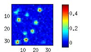
(b) Obsevation

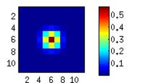
(c) True PSF

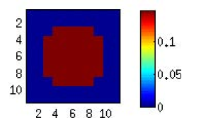
(d) Mismatched PSF

Figure 2: Experiment with Gaussian PSF: true image, observation, true PSF, and mismatched PSF ($\boldsymbol{\kappa}_{0}$).

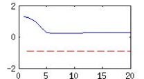
(a) $\log\|{\mathbf{y}}-{\mathrm{E}}{\mathbf{H}}{\mathrm{E}}{\mathbf{x}}\|^{2}$ (solid line) and noise level (dashed line)

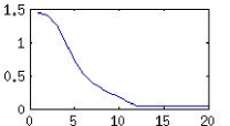
(b) $\log\|{\mathbf{x}}_{true}-{\mathrm{E}}{\mathbf{x}}\|^{2}$

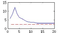
(c) ${\mathrm{E}}{\left[1/a\right]}$ (solid line) and true value (dashed line)

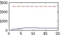
(d) ${\mathrm{E}}{\left[1/\sigma^{2}\right]}$ (solid line) and true value (dashed line)

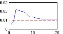
(e) ${\mathrm{E}}{\left[w\right]}$ (solid line) and true value (dashed line)

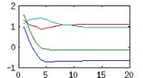
(f) ${\mathrm{E}}{\left[{\mathbf{c}}\right]}$. Four PSF coefficients.

Figure 3: Result of Algorithm 1: curves of residual, error, ${\mathrm{E}}\left[1/a\right],{\mathrm{E}}\left[1/\sigma^{2}\right],{\mathrm{E}}\left[w\right],{\mathrm{E}}\left[{\mathbf{c}}\right]$, as functions of number of iterations. These curves show how fast the convergence is achieved.

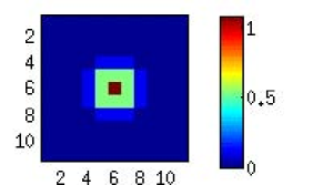
(a) Estimated PSF

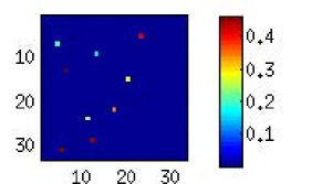
(b) Estimated image

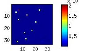
(c) Variance map

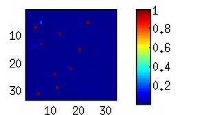
(d) Weight map

Figure 4: (a) Restored PSF, (b) image, (c) map of pixel-wise (posterior) variance, and (d) weight map. $\hat{\boldsymbol{\kappa}}={\mathrm{E}}\boldsymbol{\kappa}$ is close to the true one. A pixel-wise weight shown in (d) is the posterior probability of the pixel being a nonzero signal.

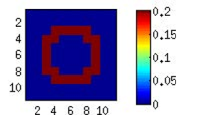
(a) The first basis $\boldsymbol{\kappa}_{1}$

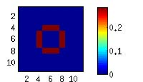
(b) The second basis $\boldsymbol{\kappa}_{2}$

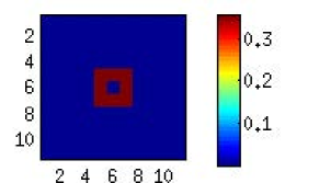
(c) The third basis $\boldsymbol{\kappa}_{3}$

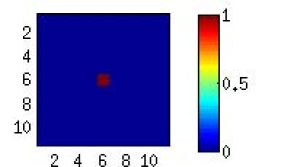
(d) The fourth basis $\boldsymbol{\kappa}_{4}$

Figure 5: PSF bases, $\boldsymbol{\kappa}_{1},\ldots,\boldsymbol{\kappa}_{4}$, for Gaussian PSF.

4.2 Simulation with MRFM type PSFs

The true image ${\mathbf{x}}$ used to generate the data, observation ${\mathbf{y}}$, the true PSF, and the initial, mismatched PSF are shown in Fig. 6. The PSF models the PSF of the MRFM instrument, derived by Mamin et al. [3]. The convergence of the algorithm is achieved after the 10th iteration. The reconstructed image can be compared to the true image in Fig. 7, where the pixel-wise variances and posterior probability of $z_{i}\neq 0$ are rendered. The PSF bases are obtained by the procedure proposed in Section 2.2 with the simplified MRFM PSF model and the nominal parameter values [10]. Specifically, by detecting a knee $K=4$ at the scree plot, explaining more than 98.69% of the observed perturbations (Fig. 3 in [9]), we use the first four eigenfunctions, corresponding to the first four largest eigenvalues. The resulting $K=4$ principal basis vectors are depicted in Fig. 8. The reconstructed PSF with the bases clearly matches the true one, as seen in Fig. 6 and Fig. 7.

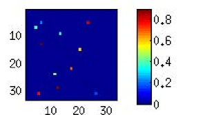
(a) True image ${\mathbf{x}}$

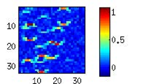
(b) Obsevation

(c) True PSF

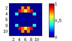
(d) Mismatched PSF

Figure 6: Experiment with simplified MRFM PSF: true image, observation, true PSF, and mismatched PSF ($\boldsymbol{\kappa}_{0}$).

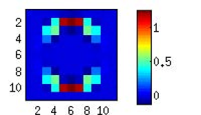
(a) Estimated PSF

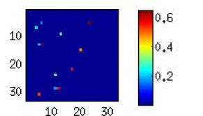
(b) Estimated image

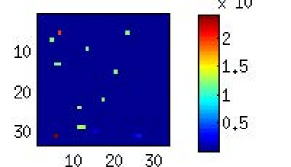
(c) Variance map

(d) Weight map

Figure 7: Restored PSF and image with pixel-wise variance and weight map. $\hat{\boldsymbol{\kappa}}={\mathrm{E}}\boldsymbol{\kappa}$ is close to the true one.

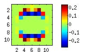
(a) The first basis $\boldsymbol{\kappa}_{1}$

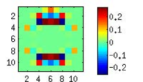
(b) The second basis $\boldsymbol{\kappa}_{2}$

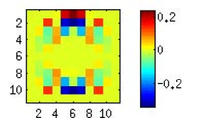
(c) The third basis $\boldsymbol{\kappa}_{3}$

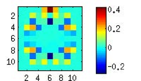
(d) The fourth basis $\boldsymbol{\kappa}_{4}$

Figure 8: PSF bases, $\boldsymbol{\kappa}_{1},\ldots,\boldsymbol{\kappa}_{4}$, for MRFM PSF.

4.3 Comparison with PSF-mismatched reconstruction

The results from the variational deconvolution algorithm with a mismatched Gaussian PSF and a MRFM type PSF are presented in Fig. 9 and Fig. 10, respectively; the relevant PSFs and observations are presented in Fig. 2 in Section 4.1 and in Fig. 6 in Section 4.2, respectively. Compared with the results of our VB semi-blind algorithm (Algorithm 1), shown in Fig. 4 and Fig. 7, the reconstructed images from the mismatched non-blind VB algorithm in Fig. 9 and Fig. 10, respectively, inaccurately estimate signal locations and blur most of the non-zero values.

Additional experiments (not shown here) establish that the PSF estimator is very accurate when the algorithm is initialized with the true image.

(a) True image

(b) Estimated image

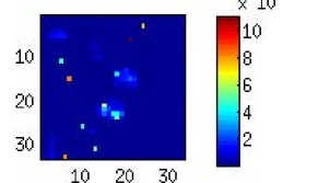
(c) Variance map

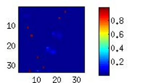
(d) Weight map

Figure 9: (mismatched) Non-blind result with a mismatched Gaussian PSF.

(a) True image

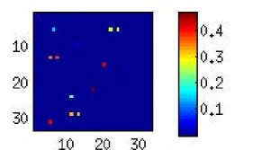
(b) Estimated image

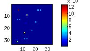
(c) Variance map

(d) Weight map

Figure 10: (mismatched) Non-blind result with a mismatched MRFM type PSF.

4.4 Comparison with other algorithms

To quantify the comparison, we performed experiments with the same set of four sparse images and the MRFM type PSFs as used in [9]. By generating 100 different noise realizations for 100 independent trials with each true image, we measured errors according to various criteria. We tested four sparse images with sparsity levels $\|{\mathbf{x}}\|_{0}=6,11,18,30$.

Under these criteria, Fig. 11 visualizes the reconstruction error performance for several measures of error. From these figures we conclude that the VB semi-blind algorithm performs at least as well as the previous MCMC semi-blind algorithm. In addition, the VB method outperforms AM [45] and the mismatched non-blind MCMC [43] methods. In terms of PSF estimation, for very sparse images the VB semi-blind method seems to outperform the MCMC method. Also, the proposed VB semi-blind method converges more quickly and requires fewer iterations. For example, the VB semi-blind algorithm converges in approximately 9.6 seconds after 12 iterations, but the previous MCMC algorithm takes more than 19.2 seconds after 40 iterations to achieve convergence.

In addition, we made comparisons between our sparse image reconstruction method and other state-of-the-art blind deconvolution methods [27, 29, 30, 28, 31, 32], as shown in our previous work [9]. These algorithms were initialized with the nominal, mismatched PSF and were applied to the same sparse image as our experiment above. For a fair comparison, we made a sparse prior modification in the image model of other algorithms, as needed. Most of these methods do not assume or fit into the sparse model in our experiments, thus leading to poor performance in terms of image and PSF estimation errors. Among these tested algorithms, two of them, proposed by Tzikas et al. [28] and Almeida et al. [30], produced non-trivial and convergent solutions and the corresponding results are compared to ours in Fig. 11. By using basis kernels the method proposed by Tzikas et al. [28] uses a similar PSF model to ours. Because a sparse image prior is not assumed in their algorithm [28], we applied their suggested PSF model along with our sparse image prior for a fair comparison. The method proposed by Almeida et al. [30] exploits the sharp edge property in natural images and uses initial, high regularization for effective PSF estimation. Both of these perform worse than our VB method as seen in Fig. 11. The remaining algorithms [27, 29, 31, 32], which focus on photo image reconstruction or motion blur, either produce a trivial solution ($\hat{\mathbf{x}}\approx{\mathbf{y}}$) or are a special case of Tzikas’s model [28].

To show lower bound our myopic reconstruction algorithm, we used the Iterative Shrinkage/Thresholding (IST) algorithm with a true PSF. This algorithm effectively restores sparse images with a sparsity constraint [46]. We demonstrate comparisons of the computation time of our proposed reconstruction algorithm to that of others in Table 1.

Table 1: Computation time of algorithms (in seconds), for the data in Fig. 6.

Our method	9.58
semi-blind MC [9]	19.20
Bayesian nonblind [43]	3.61
AM [45]	0.40
Almeida’s method [30]	5.63
Amizic’s method [29]	5.69
Tzikas’s method [28]	20.31
(oracle) IST [46]	0.09

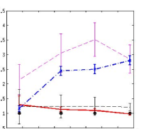
(a) $\|\hat{\mathbf{x}}\|_{0}/\|{\mathbf{x}}\|_{0}$

(b) $\|\frac{{\mathbf{x}}}{\|{\mathbf{x}}\|}-\frac{\hat{\mathbf{x}}}{\|\hat{\mathbf{x}}\|}\|_{2}^{2}/\|{\mathbf{x}}\|_{0}$

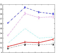
(c) $\|{\mathbf{y}}-\hat{\mathbf{y}}\|_{2}^{2}/\|{\mathbf{x}}\|_{0}$

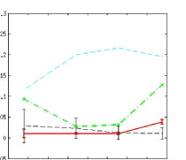
(d) $\|\frac{\hat{\boldsymbol{\kappa}}}{\|\hat{\boldsymbol{\kappa}}\|}-\frac{\boldsymbol{\kappa}}{\|\boldsymbol{\kappa}\|}\|^{2}_{2}$

Figure 11: For various image sparsity levels (x-axis: $\log_{10}\|{\mathbf{x}}\|_{0}$), performance of several blind, semi-blind, and nonblind deconvolution algorithms: the proposed method (red), AM (blue), Almeida’s method (green), Tzikas’s method (cyan), semi-blind MC (black), mismatched nonblind MC (magenta). Errors are illustrated with standard deviations. (a): Estimated sparsity. Normalized true level is $1$ (black circles). (b): Normalized error in reconstructed image. For the lower bound, information about the true PSF is only available to the oracle IST (black circles). (c): Residual (projection) error. The noise level appears in black circles. (d): PSF recovery error, as a performance gauge of our semi-blind method. At the initial stage of the algorithm, $\|\frac{\boldsymbol{\kappa}_{0}}{\|\boldsymbol{\kappa}_{0}\|}-\frac{\boldsymbol{\kappa}}{\|\boldsymbol{\kappa}\|}\|^{2}_{2}=0.5627$. (Some of the sparsity measure and residual errors are too large to be plotted together with results from other algorithms.)

4.5 Application to tobacco mosaic virus (TMV) data

We applied the proposed variational semi-blind sparse deconvolution algorithm to the tobacco mosaic virus data, made available by our IBM collaborators [38], shown in the first row in Fig. 12. Our algorithm is easily modifiable to these 3D raw image data and 3D PSF with an additional dimension in dealing with basis functions to evaluate each voxel value $x_{i}$. The noise is assumed Gaussian [36, 38] and the four PSF bases are obtained by the procedure proposed in 2.2 with the physical MRFM PSF model and the nominal parameter values [3]. The reconstruction of the 6th layer is shown in Fig. 12(b), and is consistent with the results obtained by other methods. (see [9, 43].) The estimated deviation in PSF is small, as predicted in [9].

While they now exhibit similar smoothness, the VB and MCMC images are still somewhat different since each algorithm follows different iterative trajectory in the high dimensional space of 3D images, thus converging possibly to slightly different stopping points near the maximum of the surrogate distribution. We conclude that the two images from VB and MCMC are comparable in that both represent the 2D SEM image well, but VB is significantly faster.

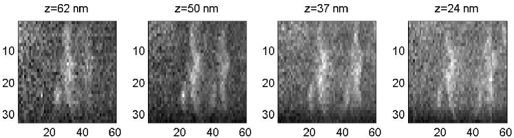
(a) TMV raw data.

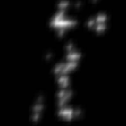
(b) VB estimate

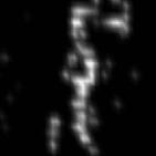
(c) MC estimate

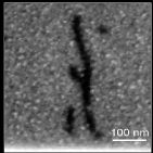
(d) SEM [38]

Figure 12: (a) TMV raw data, (b) estimated virus image by VB, (c) estimated virus image by MCMC [9], and (d) virus image from electron microscope [38].

4.6 Discussion

In blind deconvolution, joint identifiability is a common issue. For example, because of scale ambiguity, the unicity cannot be guaranteed in a general setting. It is not proven in our solution either. However, the shift/time ambiguity issue noticed in [47] is implicitly addressed in our method using a nominal and basis PSFs. Moreover, our constraint on the PSF space using a basis approach effectively excludes a delta function as a PSF solution, thus avoiding the trivial solution. Secondly, the PSF solution is restricted to this linear spanning space, starting form the initial, mismatched PSF. We can, therefore, reasonably expect that the solution provided by the algorithm is close to the true PSF, away from the trivial solution or the initial PSF.
To resolve scale ambiguity in a MCMC Bayesian framework, stochastic samplers are proposed in [47] by imposing a fixed variance on a certain distribution. Another approach to resolve the scale ambiguity is to assume a hidden scale variable that is multiplied to the PSF and dividing the image (or vice versa.), where the scale is drawn along each iteration of the Gibbs sampler [48].

5 Conclusion

We suggested a novel variational solution to a semi-blind sparse deconvolution problem. Our method uses Bayesian inference for image and PSF restoration with a sparsity-inducing image prior via the variational Bayes approximation. Its power in automatically producing all required parameter values from the data merits further attention for the extraction of image properties and retrieval of necessary features.

From the simulation results, we conclude that the performance of the VB method competes with MCMC methods in sparse image estimation, while requiring fewer computations. Compared to a non-blind algorithm whose mismatched PSF leads to imprecise and blurred signal locations in the restored image, the VB semi-blind algorithm correctly produces sparse image estimates. The benefits of this solution compared to the previous solution [9] are faster convergence and stability of the method.

Appendix A Useful Distributions

A.1 Inverse Gamma Distribution

The density of an inverse Gamma random variable $X\sim{\mathcal{I}}{\mathcal{G}}(a,b)$ is $\dfrac{b^{a}}{\Gamma(a)}x^{-a-1}\exp(-\frac{b}{x})$, for $x\in(0,\infty)$. ${\mathrm{E}}X^{-1}=a/b$ and ${\mathrm{E}}\ln(X)=\ln(b)-\psi(a)$.

A.2 Beta Distribution

The density of a Beta random variable $X\sim{\mathcal{B}}(a,b)$ is $\dfrac{\Gamma(a)\Gamma(b)}{\Gamma(a+b)}x^{b-1}(1-x)^{a-1}$, for $x\in(0,1)$, with $\Gamma(c)=\int_{0}^{\infty}t^{c-1}e^{-t}dt$. The mean of ${\mathcal{B}}(a,b)$ is $\frac{b}{a+b}$ and ${\mathrm{E}}\ln({\mathcal{B}}(a,b))=\psi(b)-\psi(a+b)$, where $\psi$ is a digamma function.

A.3 Positively Truncated Gaussian Distribution

The density of a truncated Gaussian random variable $x_{i}$ is denoted by $x_{i}\sim{\mathcal{N}}_{+}(x_{i};\mu,\eta)$, and its statistics used in the paper are

$${\mathrm{E}}\left[x_{i}|x_{i}>0\right] ={\mathrm{E}}\left[{\mathcal{N}}_{+}(x_{i};\mu,\eta)\right]$$

$$=\mu+\sqrt{\eta}\frac{\phi(-\mu/\sqrt{\eta})}{1-\Phi_{0}(-\mu/\sqrt{\eta})},$$

$${\mathrm{E}}\left[x_{i}^{2}|x_{i}>0\right] =\mathrm{var}[x_{i}|x_{i}>0]+({\mathrm{E}}\left[x_{i}|x_{i}>0\right])^{2}$$

$$=\eta+\mu({\mathrm{E}}\left[x_{i}|x_{i}>0\right]),$$

where $\Phi_{0}$ is a cumulative distribution function for the standard normal distribution.

Appendix B Derivations of $q(\cdot)$

In this section, we derive the posterior densities defined by variational Bayes framework in Section 3.

B.1 Derivation of $q({\mathbf{c}})$

We denote the expected value of the squared residual term by $R={\mathrm{E}}\|{\mathbf{y}}-{\mathbf{H}}{\mathbf{x}}\|^{2}$. For $c_{l},l=1,\ldots,K$,

$$R= {\mathrm{E}}\|{\mathbf{y}}-{\mathbf{H}}^{0}{\mathbf{x}}-\sum_{l\neq j}{\mathbf{H}}^{l}{\mathbf{x}}c_{l}-{\mathbf{H}}^{j}{\mathbf{x}}c_{j}\|^{2}$$

$$= c_{j}^{2}\langle{\mathbf{x}}^{T}{{\mathbf{H}}^{j}}^{T}{\mathbf{H}}^{j}{\mathbf{x}}\rangle-2c_{j}\langle{\mathbf{x}}^{T}{{\mathbf{H}}^{j}}^{T}{\mathbf{y}}-{\mathbf{x}}{{\mathbf{H}}^{j}}^{T}{\mathbf{H}}^{0}{\mathbf{x}}$$

$$-\sum_{l\neq j}{\mathbf{x}}^{T}{{\mathbf{H}}^{j}}^{T}{\mathbf{H}}^{l}c_{l}{\mathbf{x}}\rangle+\mathrm{const},$$

where ${\mathbf{H}}^{j}$ is the convolution matrix corresponding to the convolution with $\boldsymbol{\kappa}_{j}$. For $i\neq j$ and $i,j>0$, ${\mathrm{E}}({\mathbf{H}}^{i}{\mathbf{x}})^{T}({\mathbf{H}}^{j}{\mathbf{x}})=tr({{\mathbf{H}}^{i}}^{T}{\mathbf{H}}^{j}(\mathrm{cov}({\mathbf{x}})+\langle{\mathbf{x}}\rangle\langle{\mathbf{x}}^{T}\rangle))=({\mathbf{H}}^{i}\langle{\mathbf{x}}\rangle)^{T}({\mathbf{H}}^{j}\langle{\mathbf{x}}\rangle)$, since $tr({{\mathbf{H}}^{i}}^{T}{\mathbf{H}}^{j}\mathrm{cov}({\mathbf{x}}))=tr({{\mathbf{H}}^{i}D}^{T}{\mathbf{H}}^{j}D)=\sum_{k}d_{k}^{2}{\mathbf{h}}_{k}^{i}{\mathbf{h}}_{k}^{j}=0$. Here, $\mathrm{cov}({\mathbf{x}})$ is approximated as a diagonal matrix $D^{2}=\mathrm{diag}(d_{1}^{2},\ldots,d_{n}^{2})$. This is reasonable, especially when the expected recovered signal $\hat{\mathbf{x}}$ exhibits high sparsity. Likewise, ${\mathrm{E}}({\mathbf{H}}^{0}{\mathbf{x}})^{T}({\mathbf{H}}^{j}{\mathbf{x}})=\boldsymbol{\kappa}_{0}^{T}\boldsymbol{\kappa}_{j}\sum_{i}\mathrm{var}[x_{i}]+({\mathbf{H}}^{0}\langle{\mathbf{x}}\rangle)^{T}({\mathbf{H}}^{j}\langle{\mathbf{x}}\rangle)$ and ${\mathrm{E}}({\mathbf{H}}^{j}{\mathbf{x}})^{T}({\mathbf{H}}^{j}{\mathbf{x}})=\|\boldsymbol{\kappa}_{j}\|^{2}\sum_{i}\mathrm{var}[x_{i}]+\|{\mathbf{H}}^{j}\langle{\mathbf{x}}\rangle\|^{2}$.

Then, we factorize ${\mathrm{E}}\left[-\frac{R}{2\sigma^{2}}\right]=-\frac{(c_{j}-\mu_{c_{j}})^{2}}{2\sigma_{c_{j}}}$, with $\mu_{c_{j}}=\frac{\langle{\mathbf{x}}^{T}{{\mathbf{H}}^{j}}^{T}{\mathbf{y}}-{\mathbf{x}}{{\mathbf{H}}^{j}}^{T}{\mathbf{H}}^{0}{\mathbf{x}}-\sum_{l\neq j}{\mathbf{x}}^{T}{{\mathbf{H}}^{j}}^{T}{\mathbf{H}}^{l}c_{l}{\mathbf{x}}\rangle}{\langle{\mathbf{x}}^{T}{{\mathbf{H}}^{j}}^{T}{\mathbf{H}}^{j}{\mathbf{x}}\rangle}$, $1/\sigma_{c_{j}}=\langle 1/\sigma^{2}\rangle\langle{\mathbf{x}}^{T}{{\mathbf{H}}^{j}}^{T}{\mathbf{H}}^{j}{\mathbf{x}}\rangle$.

If we set the prior, $p(c_{j})$, to be a uniform distribution over a wide range of the real line that covers error tolerances, we obtain a normally distributed variational density $q(c_{j})=\phi(\mu_{c_{j}},\sigma_{c_{j}})$ with its mean $\mu_{c_{j}}$ and variance $\sigma_{c_{j}}$ defined above, because $\ln q(c_{j})={\mathrm{E}}\left[-\frac{R}{2\sigma^{2}}\right]$. By the independence assumption, $q({\mathbf{c}})=\prod q(c_{j})$, so $q({\mathbf{c}})$ can be easily evaluated.

B.2 Derivation of $q(\sigma^{2})$

We evaluate $R$ ignoring edge effects; $R=\|{\mathbf{y}}-\langle{\mathbf{H}}\rangle\langle{\mathbf{x}}\rangle\|^{2}+\sum\mathrm{var}[x_{i}][\|\langle\boldsymbol{\kappa}\rangle\|^{2}+\sum_{l}\sigma_{c_{l}}\|\boldsymbol{\kappa}_{l}\|^{2}]+\sum_{l}\sigma_{c_{l}}\|{{\mathbf{H}}^{l}\langle{\mathbf{x}}\rangle}\|^{2}$. $\|\boldsymbol{\kappa}\|^{2}$ is a kernel energy in $\ell_{2}$ sense and the variance terms add uncertainty, due to the uncertainty in $\boldsymbol{\kappa}$, to the estimation of density. Applying (19), (ignoring constants)

$$\ln q(\sigma^{2}) ={\mathrm{E}}_{\backslash\sigma^{2}}\left[\ln p({\mathbf{y}}|{\mathbf{x}},{\mathbf{c}},\sigma^{2})p(\sigma^{2})p({\mathbf{x}}|a,w)p(w)p(a)\right]$$

$$={\mathrm{E}}_{{\mathbf{x}},{\mathbf{c}}}\left[\ln p({\mathbf{y}}|{\mathbf{x}},\sigma^{2})\right]+\ln p(\sigma^{2})$$

$$=-\frac{{\mathrm{E}}_{{\mathbf{x}},{\mathbf{c}}}\left[\|{\mathbf{y}}-{\mathbf{H}}{\mathbf{x}}\|^{2}\right]}{2\sigma^{2}}-\frac{P}{2}\ln\sigma^{2}+\ln p(\sigma^{2}).$$

$${\mathcal{I}}{\mathcal{G}}(\tilde{\varsigma}_{0},\tilde{\varsigma}_{1}) \triangleq q(\sigma^{2})={\mathcal{I}}{\mathcal{G}}(P/2+\varsigma_{0},\langle\|{\mathbf{y}}-{\mathbf{H}}{\mathbf{x}}\|^{2}\rangle/2+\varsigma_{1}).$$

(${\mathrm{E}}_{\backslash\sigma^{2}}$ denotes expectation with respect to all variables except $\sigma^{2}$.)

B.3 Derivation of $q({\mathbf{x}})$

For $x_{i},i=1,\ldots,N$, $R={\mathrm{E}}\|{\mathbf{e}}_{i}-{\mathbf{h}}_{i}x_{i}\|^{2}$ with ${\mathbf{e}}_{i}={\mathbf{y}}-{\mathbf{H}}{\mathbf{x}}_{-i}={\mathbf{y}}-{\mathbf{H}}^{0}{\mathbf{x}}_{-i}-\sum_{l}{\mathbf{H}}^{l}c_{l}{\mathbf{x}}_{-i}$, ${\mathbf{h}}_{i}=[{\mathbf{H}}^{0}+\sum{\mathbf{H}}^{l}c_{l}]_{i}={\mathbf{h}}^{0}_{i}+\sum{\mathbf{h}}^{l}_{i}c_{l}=$ ($i$th column of ${\mathbf{H}}$). Ignoring constants, $R=\langle\|{\mathbf{h}}_{i}\|^{2}\rangle x_{i}^{2}-2\langle{\mathbf{h}}_{i}^{T}{\mathbf{e}}_{i}\rangle x_{i}$.

Using the orthogonality of the kernel bases and uncorrelatedness of $c_{l}$’s, we derive the following terms (necessary to evaluate $R$): $\langle\|{\mathbf{h}}_{i}\|^{2}\rangle=\|{\mathbf{h}}^{0}_{i}\|^{2}+\sum_{l}\sigma_{c_{l}}\|{{\mathbf{h}}^{l}}_{i}\|^{2}$ and, $\langle{\mathbf{h}}_{i}^{T}{\mathbf{e}}_{i}\rangle=\langle{\mathbf{h}}_{i}^{T}\rangle({\mathbf{y}}-\langle{\mathbf{H}}\rangle\langle{\mathbf{x}}_{-i}\rangle)-\sum_{l}\mathrm{var}[c_{l}]{{\mathbf{h}}^{l}_{i}}^{T}{\mathbf{H}}^{l}\langle{\mathbf{x}}_{-i}\rangle$.

Then, $\mathrm{var}[x_{i}]=w_{i}^{\prime}{\mathrm{E}}\left[x_{i}^{2}|x_{i}>0\right]-w_{i}^{\prime 2}({\mathrm{E}}\left[x_{i}|x_{i}>0\right])^{2}$, ${\mathrm{E}}\left[x_{i}\right]=w_{i}^{\prime}{\mathrm{E}}\left[x_{i}|x_{i}>0\right]$, where $w_{i}^{\prime}=q(z_{i}=1)$ is the posterior weight for the normal distribution and $1-w_{i}^{\prime}$ is the weight for the delta function. The required statistics of $x_{i}$ that are used to derive the distribution above are obtained by applying A.3.

B.4 Derivation of $q({\mathbf{z}})$

To derive $q(z_{i}=1)=\langle z_{i}\rangle$, we evaluate the unnormalized version $\hat{q}(z_{i})$ of $q(z_{i})$ and normalize it. $\ln\hat{q}(z_{i}=1)={\mathrm{E}}_{\backslash z_{i}}\left[-\frac{\|{\mathbf{e}}_{i}-{\mathbf{h}}_{i}x_{i}\|^{2}}{2\sigma^{2}}-\ln a-\frac{x_{i}}{a}+\ln w\right]$ with ${x_{i}\sim N_{+}(\mu_{i},\eta_{i})}$ and $\ln\hat{q}(z_{i}=0)={\mathrm{E}}_{\backslash z_{i}}\left[-\frac{\|{\mathbf{e}}_{i}\|^{2}}{2\sigma^{2}}+\ln(1-w)\right]$ with ${x_{i}=0}$. The normalized version of the weight is $q(z_{i}=1)={1}/[{1+C^{\prime}_{i}}]$. $C^{\prime}_{i}=\exp(\ln\hat{q}(z_{i}=0)-\ln\hat{q}(z_{i}=1))=\exp(C_{i}/2\times\langle 1/\sigma^{2}\rangle+\mu\langle 1/a\rangle+\langle\ln a\rangle+\langle\ln(1-w)-\ln w\rangle=\exp(C_{i}/2\times\tilde{\varsigma}_{0}/\tilde{\varsigma}_{1}+\mu\tilde{\alpha}_{0}/\tilde{\alpha}_{1}+\ln\tilde{\alpha}_{1}-\psi(\tilde{\alpha}_{0})+\psi(\tilde{\beta}_{0})-\psi(\tilde{\beta}_{1}))$. $\psi$ is a digamma function and $C_{i}=\langle\|{\mathbf{h}}_{i}\|^{2}\rangle(\mu_{i}^{2}+\eta_{i})-2\langle{\mathbf{e}}_{i}^{T}{\mathbf{h}}_{i}\rangle\mu_{i}$.

References

- [1] R. Ward, B. Saleh, Deblurring random blur, IEEE Trans. Acoustics, Speech, Signal Processing 35 (10) (1987) 1494–1498.
- [2] D. Kundur, D. Hatzinakos, Blind image deconvolution, IEEE Signal Processing Magazine 13 (3) (1996) 43–64.
- [3] J. Mamin, R. Budakian, D. Rugar, Point response function of an MRFM tip, Tech. rep., IBM Research Division (Oct. 2003).
- [4] S. Makni, P. Ciuciu, J. Idier, J.-B. Poline, Joint detection-estimation of brain activity in functional mri: A multichannel deconvolution solution, IEEE Trans. Signal Processing 53 (9) (2005) 3488–3502.
- [5] G. Pillonetto, C. Cobelli, Identifiability of the stochastic semi-blind deconvolution problem for a class of time-invariant linear systems, Automatica 43 (4) (2007) 647–654.
- [6] P. Sarri, G. Thomas, E. Sekko, P. Neveux, Myopic deconvolution combining Kalman filter and tracking control, in: Proc. IEEE Int. Conf. Acoust., Speech, and Signal (ICASSP), Vol. 3, 1998, pp. 1833–1836.
- [7] G. Chenegros, L. M. Mugnier, F. Lacombe, M. Glanc, 3D phase diversity: a myopic deconvolution method for short-exposure images: application to retinal imaging, J. Opt. Soc. Am. A 24 (5) (2007) 1349–ÃÂ1357.
- [8] S. U. Park, N. Dobigeon, A. O. Hero, Myopic sparse image reconstruction with application to MRFM, in: C. A. Bouman, I. Pollak, P. J. Wolfe (Eds.), Proc. Computational Imaging Conference in IS&T SPIE Symposium on Electronic Imaging Science and Technology, Vol. 7873, SPIE, 2011, pp. 787303/1–787303/14.
- [9] S. U. Park, N. Dobigeon, A. O. Hero, Semi-blind sparse image reconstruction with application to MRFM, IEEE Trans. Image Processing 21 (9) (2012) 3838 –3849.
- [10] M. Ting, R. Raich, A. O. Hero, Sparse image reconstruction for molecular imaging, IEEE Trans. Image Processing 18 (6) (2009) 1215–1227.
- [11] C. M. Bishop, Pattern Recognition and Machine Learning, Springer, New York, NY, USA, 2006.
- [12] N. Nasios, A. Bors, Variational learning for Gaussian mixture models, IEEE Trans. Systems, Man, Cybernet. Part B 36 (4) (2006) 849–862.
- [13] A. Corduneanu, C. M. Bishop, Variational Bayesian model selection for mixture distributions, in: Proc. Conf. Artificial Intelligence and Statistics, 2001, pp. 27–34.
- [14] K. Themelis, A. Rontogiannis, K. Koutroumbas, A novel hierarchical Bayesian approach for sparse semisupervised hyperspectral unmixing, IEEE Trans. Signal Processing 60 (2) (2012) 585–599.
- [15] S. Makni, J. Idier, T. Vincent, B. Thirion, G. Dehaene-Lambertz, P. Ciuciu, A fully Bayesian approach to the parcel-based detection-estimation of brain activity in fMRI., Neuroimage.
- [16] C. P. Robert, G. Casella, Monte Carlo Statistical Methods, 2nd Edition, Springer, 2004.
- [17] W. R. Gilks, Markov Chain Monte Carlo In Practice, Chapman and Hall/CRC, 1999.
- [18] F. Orieux, J.-F. Giovannelli, T. Rodet, Bayesian estimation of regularization and point spread function parameters for Wiener-Hunt deconvolution, J. Opt. Soc. Am. A 27 (7) (2010) 1593–1607.
- [19] H. Attias, A variational Bayesian framework for graphical models, in: Proc. Adv. in Neural Inf. Process. Syst. (NIPS), MIT Press, 2000, pp. 209–215.
- [20] A. M. Walker, On the asymptotic behaviour of posterior distributions, Journal of the Royal Statistical Society. Series B (Methodological) 31 (1) (1969) 80–88.
- [21] B. Wang, D. Titterington, Convergence and asymptotic normality of variational Bayesian approximations for exponential family models with missing values, in: Proc. Conf. Uncertainty in Artificial Intelligence (UAI), AUAI Press, 2004, pp. 577–584.
- [22] B. Wang, M. Titterington, Convergence properties of a general algorithm for calculating variational Bayesian estimates for a normal mixture model, Bayesian Anal. 1 (3) (2006) 625–650.
- [23] C. M. Bishop, J. M. Winn, C. C. Nh, Non-linear Bayesian image modelling, in: Proc. Eur. Conf. Comput. Vis. (EECV), Springer-Verlag, 2000, pp. 3–17.
- [24] Z. Ghahramani, M. J. Beal, Variational inference for Bayesian mixtures of factor analysers, in: Proc. Adv. in Neural Inf. Process. Syst. (NIPS), MIT Press, 2000, pp. 449–455.
- [25] M. J. Beal, Z. Ghahramani, The variational Bayesian EM algorithm for incomplete data: with application to scoring graphical model structures, in: Bayesian Stat., Vol. 7, 2003, pp. 453–464.
- [26] J. Winn, C. M. Bishop, T. Jaakkola, Variational message passing, Journal of Machine Learning Research 6 (2005) 661–694.
- [27] S. Babacan, R. Molina, A. Katsaggelos, Variational Bayesian blind deconvolution using a total variation prior, IEEE Trans. Image Processing 18 (1) (2009) 12–26.
- [28] D. Tzikas, A. Likas, N. Galatsanos, Variational Bayesian sparse kernel-based blind image deconvolution with Student’s-t priors, IEEE Trans. Image Processing 18 (4) (2009) 753–764.
- [29] B. Amizic, S. D. Babacan, R. Molina, A. K. Katsaggelos, Sparse Bayesian blind image deconvolution with parameter estimation, in: Proc. Eur. Signal Process. Conf. (EUSIPCO), Aalborg (Denmark), 2010, pp. 626–630.
- [30] M. Almeida, L. Almeida, Blind and semi-blind deblurring of natural images, IEEE Trans. Image Processing 19 (1) (2010) 36–52.
- [31] R. Fergus, B. Singh, A. Hertzmann, S. T. Roweis, W. T. Freeman, Removing camera shake from a single photograph, in: ACM SIGGRAPH 2006 Papers, SIGGRAPH ’06, ACM, New York, NY, USA, 2006, pp. 787–794.
- [32] Q. Shan, J. Jia, A. Agarwala, High-quality motion deblurring from a single image, ACM Trans. Graphics 27 (3) (2008) 1.
- [33] J. A. Sidles, Noninductive detection of single-proton magnetic resonance, Appl. Phys. Lett. 58 (24) (1991) 2854–2856.
- [34] J. A. Sidles, Folded stern-gerlach experiment as a means for detecting nuclear magnetic resonance in individual nuclei, Phys. Rev. Lett. 68 (8) (1992) 1124–1127.
- [35] J. A. Sidles, J. L. Garbini, K. J. Bruland, D. Rugar, O. Züger, S. Hoen, C. S. Yannoni, Magnetic resonance force microscopy, Rev. Mod. Phys. 67 (1) (1995) 249–265.
- [36] D. Rugar, C. S. Yannoni, J. A. Sidles, Mechanical detection of magnetic resonance, Nature 360 (6404) (1992) 563–566.
- [37] O. Züger, S. T. Hoen, C. S. Yannoni, D. Rugar, Three-dimensional imaging with a nuclear magnetic resonance force microscope, J. Appl. Phys. 79 (4) (1996) 1881–1884.
- [38] C. L. Degen, M. Poggio, H. J. Mamin, C. T. Rettner, D. Rugar, Nanoscale magnetic resonance imaging, Proc. Nat. Academy of Science 106 (5) (2009) 1313–1317.
- [39] O. Züger, D. Rugar, First images from a magnetic resonance force microscope, Applied Physics Letters 63 (18) (1993) 2496–2498.
- [40] O. Züger, D. Rugar, Magnetic resonance detection and imaging using force microscope techniques, J. Appl. Phys. 75 (10) (1994) 6211–6216.
- [41] S. Chao, W. M. Dougherty, J. L. Garbini, J. A. Sidles, Nanometer-scale magnetic resonance imaging, Review Sci. Instrum. 75 (5) (2004) 1175–1181.
- [42] C. L. Degen, M. Poggio, H. J. Mamin, C. T. Rettner, D. Rugar, Nanoscale magnetic resonance imaging. Supporting information, Proc. Nat. Academy of Science 106 (5).
- [43] N. Dobigeon, A. O. Hero, J.-Y. Tourneret, Hierarchical Bayesian sparse image reconstruction with application to MRFM, IEEE Trans. Image Processing 18 (9) (2009) 2059–2070.
- [44] L. Landweber, An iteration formula for Fredholm integral equations of the first kind, Amer. J. Math. 73 (3) (1951) 615–624.
- [45] K. Herrity, R. Raich, A. O. Hero, Blind deconvolution for sparse molecular imaging, in: Proc. IEEE Int. Conf. Acoust., Speech, and Signal (ICASSP), Las Vegas, USA, 2008, pp. 545–548.
- [46] I. Daubechies, M. Defrise, C. De Mol, An iterative thresholding algorithm for linear inverse problems with a sparsity constraint, Communications on Pure and Applied Mathematics 57 (11) (2004) 1413–1457.
- [47] D. Ge, J. Idier, E. L. Carpentier, Enhanced sampling schemes for MCMC based blind Bernoulli–Gaussian deconvolution, Signal Processing 91 (4) (2011) 759 –772.
- [48] T. Vincent, L. Risser, P. Ciuciu, Spatially adaptive mixture modeling for analysis of fMRI time series, IEEE Trans. Med. Imag. 29 (4) (2010) 1059–1074.