Higgs decay into diphoton in the Composite Higgs Model

Abstract

We explore the Higgs couplings to gauge bosons in the minimal $SO(5)/SO(4)$ 4D composite Higgs model. The pion scatterings put unitary constraints on the couplings and therefore determine the branching ratios of various Higgs decays. Through fine-tuning the parameters, enhancement of Higgs to diphoton rate is possible to be achieved with the existence of vector meson fields.

1 Introduction

The composite Higgs model provides an alternative solution to the little hierarchy problem compared with the well-known supersymmetric models, since the economic formulation of the standard model is impossible to explain the lightness of Higgs mass. The composite Higgs boson emerges as a pseudo-Nambu-Goldstone boson (pNGB) from a spontaneously broken global symmetry, therefore its mass is much lighter than the other resonances from the strong dynamic sector. The original minimal composite model is realized in the five-dimensional Randall Sundrum model, and the Higgs is the fifth component of the broken gauge bosons [1]. Using the holographic approaching, the effective Lagrangian is gained after integrating out the bulk field with the UV brane value fixed. The potential for the holographic composite Higgs could be calculated in the form of brane to brane 5D propagators [2]. In the last few years increased attention has been focused on the deconstruction version of the 5D theory, which leads to varieties of 4D composite Higgs models, assuming the existence of one elementary sector and one strong interaction sector [3]. Without the presence of additional composite fields, the composite Higgs has a reduced coupling with the gauge bosons, which may lead to the violation of unitary in the pion scatterings before the cutoff scale is reached. The method to restore the perturbative unitary is to introduce vector resonances. The unitary requirement will correlate the global symmetry breaking scale $f$ with the mass $m_{\rho}$ of the vector resonance. It is interesting that the presence of the vector resonance will also modify the Higgs coupling, with its deviation parametrized by $\xi=v^{2}/f^{2}$, which in turn changes the branching ratio of various Higgs decay. Another crucial ingredient in the composite Higgs model is the partial compositeness of gauge bosons due to the nonlinearity, with the degree of compositeness mainly controlled by the gauge couplings. In this paper we first review a simple model setup of 4D composite Higgs and show that it is capable to accommodate the $125~{}\mbox{GeV}$ resonance with the appropriate properties recently discovered at the LHC [4].

2 Lagrangian of the sigma model

Let us start with the basic model setup. Our Higgs is realized as one pNGB from a strong interacting sector using the nonlinear sigma model. We formulate the effective Lagrangian for those pNGBs via the Callan-Coleman-Wess-Zumino (CCWZ) prescription [5]. In the following, we are going to review the nonlinear realization of composite Higgs and capture the necessary ingredients for our calculations. Considering the global symmetry breaking pattern $SO(5)\to SO(4)$, there are four pNGBs which fit a basic representation of the $SO(4)$ symmetry group. The first three, i.e. $\pi_{1,2,3}$, are eaten by the $W,Z$ bosons, with the remaining one, $\pi_{4}$, identified as the Higgs. Denoting the Goldstone bosons as $U=exp(i\sqrt{2}\pi^{\hat{a}}T^{\hat{a}}/f)$, the sigma field would transform nonlinearly under the full global symmetry as $U\to gUh^{\dagger}(g,\pi)$, and one can calculate the structure of $iU^{\dagger}\partial_{\mu}U=d_{\mu}^{\hat{a}}T^{\hat{a}}+E_{\mu}^{a_{L}}T^{a_{L}}+E_{\mu}^{a_{R}}T^{a_{R}}$, where $T^{\hat{a}},\hat{a}=1,2,3,4$ are the broken generators in the coset space of $SO(5)/SO(4)$, and $T^{a_{L}(a_{R})},a_{L}(a_{R})=1,2,3$ are the unbroken generators in the $SO(4)\simeq SU(2)_{L}\times SU(2)_{R}$ symmetry group. It should be noted that all the generators in the $SO(5)$ symmetry group are normalized as $\mbox{Tr}(T^{a}T^{b})=\delta^{ab}$. The building blocks of the CCWZ formalism are the variables $d_{\mu}^{\hat{a}}$ and $E_{\mu}^{a_{L},a_{R}}$ decomposed in the broken and unbroken generator directions respectively. Following the usual formulation, we gauge a subgroup $SU(2)\times U(1)$ in the global $SO(4)$, resulting in an explicit breaking of the full global symmetry. The gauged CCWZ structures are calculated in a similar approach by substituting $\partial_{\mu}$ with the covariant operator $D_{\mu}=\partial_{\mu}-ig_{0}W_{\mu}^{a}T_{L}^{a}-iB_{\mu}T_{R}^{3}$. At the leading order of the chiral expansion, $d_{\mu}^{\hat{a}}$ and $E_{\mu}^{a_{L},a_{R}}$ are expressed as:

$$d_{\mu}^{\hat{a}} = -\frac{\sqrt{2}}{f}D_{\mu}\pi^{\hat{a}}+\frac{\sqrt{2}}{3f^{3}}{\left[\pi,\left[\pi,D_{\mu}\pi\right]\right]^{\hat{a}}}+\cdots\,,$$ (1)

$$E_{\mu}^{a} = g_{0}W_{\mu}^{a}+{g^{\prime}}_{0}B_{\mu}\delta^{a3}+\frac{i}{f^{2}}{\left[\pi,D_{\mu}\pi\right]^{a}}+\cdots$$ (2)

under the local symmetry group, the corresponding transformation rules are:

$$d_{\mu}\to h(g,\pi)d_{\mu}h^{\dagger}(g,\pi),\quad E_{\mu}\to h(g,\pi)E_{\mu}h^{\dagger}(g,\pi)+ih(g,\pi)\partial_{\mu}h^{\dagger}(g,\pi)$$ (3)

since $E_{\mu}$ behaves as a gauge field, the coupling of Goldstone bosons to the fundamental fermions is via the covariant derivative $\partial_{\mu}-iE_{\mu}$. In this paper we are only concerned with the vector meson effects and would not explore too much into the fermion sector. We can conveniently calculate the mass terms for the $W$ and $Z$ gauge bosons after electroweak symmetry breaking through the kinetic terms:

$$\frac{f^{2}}{4}\mbox{Tr}~{}{d^{\mu}}{d_{\mu}}=\frac{1}{2}\frac{2m_{W}^{2}}{v}(v+2ah+b\frac{h^{2}}{v})W_{\mu}^{+}W_{\mu}^{-}+\frac{1}{2}\frac{m_{Z}^{2}}{v}(v+2ah+b\frac{h^{2}}{v})Z_{\mu}Z_{\mu}+\mathcal{O}(h^{3})~{}$$ (4)

$$m_{W}^{2}=\frac{g_{0}^{2}{f^{2}}\sin{\theta^{2}}}{4},~{}m_{Z}^{2}=\frac{(g_{0}^{2}+g_{0}^{\prime 2}){f^{2}}\sin{\theta^{2}}}{4},~{}a=\cos\theta,~{}b=\cos^{2}\theta-\sin^{2}\theta$$ (5)

where the parameters $a$ and $b$, both of which are always less than one, indicate that the Higgs couplings are reduced as compared with the Standard Model. In the minimal $SO(5)/SO(4)$ setup, $\theta$ is the misalignment of the true vacuum relative to the gauged $SO(4)$ subgroup, with the VEV of the Higgs defined as $v=f\sin\theta=246.0~{}\mbox{GeV}$.

Under the partial UV completion hypothesis [6], one pair of $\rho_{L\mu}$ and $\rho_{R\mu}$ in the representations $(3,1)\oplus(1,3)$ of $SU(2)_{L}\times SU(2)_{R}$, transforming under the local symmetry group as $\rho\to h(g,\pi)\rho_{\mu}h^{\dagger}(g,\pi)+ih(g,\pi)\partial_{\mu}h^{\dagger}(g,\pi)$, needs to be added into the strong dynamic sector. The gauge invariant Lagrangian for the vector resonances consisting of kinetic terms and mass terms is formulated as:

$$\mathcal{L}_{\rho L} = -\frac{1}{4}\mbox{Tr}\left({{\rho_{L,\mu\nu}}\rho_{L}^{\mu\nu}}\right)+\frac{{a_{\rho_{L}}^{2}f^{2}}}{2}\mbox{Tr}{\left({{g_{\rho_{L}}}{\rho_{L\mu}}-E_{\mu}^{L}}\right)^{2}}\,,$$ (6)

$$\mathcal{L}_{\rho R} = -\frac{1}{4}\mbox{Tr}\left({{\rho_{R,\mu\nu}}\rho_{R}^{\mu\nu}}\right)+\frac{{a_{\rho_{R}}^{2}f^{2}}}{2}\mbox{Tr}{\left({{g_{\rho_{R}}}{\rho_{R\mu}}-E_{\mu}^{R}}\right)^{2}}\,.$$ (7)

At the low energy scale, we are only interested in the interactions which are relevant to the pion scatterings, that is the Goldstone bosons self-interactions and at most their interactions with the vector resonances. After a little bit of algebra, it is easy to reach the explicit Lagrangian:

$$\mathcal{L}_{\rho_{L}\pi^{2}+\pi^{4}} = \frac{{a_{\rho L}^{2}{g_{\rho L}}}}{2}\left[{{\varepsilon^{ijk}}{\pi^{i}}{\partial_{\mu}}{\pi^{j}}\rho_{L\mu}^{k}+\left({{\pi^{k}}{\partial_{\mu}}{\pi^{4}}-{\pi^{4}}{\partial_{\mu}}{\pi^{k}}}\right)\rho_{L\mu}^{k}}\right]$$ (8)

$$-\frac{{a_{\rho L}^{2}}}{{8{f^{2}}}}\left[{{{\left({{\pi^{a}}{\partial_{\mu}}{\pi^{a}}}\right)}^{2}}-{{\left({{\pi^{a}}{\partial_{\mu}}{\pi^{b}}}\right)}^{2}}}\right]$$

$$\mathcal{L}_{\rho_{R}\pi^{2}+\pi^{4}} = \frac{{a_{\rho R}^{2}{g_{\rho R}}}}{2}\left[{{\varepsilon^{ijk}}{\pi^{i}}{\partial_{\mu}}{\pi^{j}}\rho_{R\mu}^{k}-\left({{\pi^{k}}{\partial_{\mu}}{\pi^{4}}-{\pi^{4}}{\partial_{\mu}}{\pi^{k}}}\right)\rho_{R\mu}^{k}}\right]$$ (9)

$$-\frac{{a_{\rho R}^{2}}}{{8{f^{2}}}}\left[{{{\left({{\pi^{a}}{\partial_{\mu}}{\pi^{a}}}\right)}^{2}}-{{\left({{\pi^{a}}{\partial_{\mu}}{\pi^{b}}}\right)}^{2}}}\right]$$

Since the $h\pi^{2}$ and $h^{2}\pi^{2}$ interactions are determined by $a$ and $b$, whereas the pion self-interaction and pion interaction with vector meson are related to $a_{\rho}$ and the global symmetry breaking scale $f$, the correlation between those parameters and the allowed parameter space information could be extracted from both the pion elastic and the pion inelastic scatterings.

3 Consider Elastic and Inelastic Pion Scattering

3.1 $\pi\pi\to\pi\pi$ scattering

For the scattering $\pi^{a}\pi^{b}\to\pi^{c}\pi^{d}$ of the $SU(2)$-triplet Goldstones, the amplitude has the general isospin structure:

$$A({\pi^{a}}{\pi^{b}}\to{\pi^{c}}{\pi^{d}})=A(s,t,u)^{(\pi\pi)}\delta^{ab}\delta^{cd}+A(t,s,u)^{(\pi\pi)}\delta^{ac}\delta^{bd}+A(u,t,s)^{(\pi\pi)}\delta^{ad}\delta^{bc}$$ (10)

$$A(s,t,u)^{(\pi\pi)}=\frac{s}{v^{2}}-\frac{a_{\rho L}^{2}}{4f^{2}}\left[{3s+m_{\rho L}^{2}\left({\frac{{s-u}}{{t-m_{\rho L}^{2}}}+\frac{{s-t}}{{u-m_{\rho L}^{2}}}}\right)}\right]$$

$$\qquad-\frac{a_{\rho R}^{2}}{4f^{2}}\left[{3s+m_{\rho R}^{2}\left({\frac{s-u}{t-m_{\rho R}^{2}}+\frac{s-t}{u-m_{\rho R}^{2}}}\right)}\right]-\frac{a^{2}}{v^{2}}\frac{s^{2}}{s-m_{h}^{2}}$$ (11)

where the terms with dependence on the mass $m_{\rho_{L,R}}$ comes from $\rho_{L,R}$ meson mediated $t$ channel and $u$ channel diagrams, and the last term comes from the light Higgs mediated $s$ channel diagram, whereas the remaining terms come from the contact interaction. The amplitude can be decomposed into $1,3,5$ in the isospin basis:

$$T_{0}(s,t,u) = 3A(s,t,u)+A(t,s,u)+A(u,t,s),$$ (12)

$$T_{1}(s,t,u) = A(t,s,u)-A(u,t,s),$$ (13)

$$T_{2}(s,t,u) = A(t,s,u)+A(u,t,s)\,.$$ (14)

It is then possible to transform these isospin amplitudes in terms of the partial wave (PW) decomposition

$$T^{I}(s,t)\,=\,\sum_{J=0}^{\infty}32\pi\,(2J+1)\,P_{J}(\cos\alpha)\,a^{I}_{J}(s)\,,$$ (15)

with the partial waves provided by

$$a^{I}_{J}(s)\,=\,\frac{\displaystyle 1}{\displaystyle 64\pi}\,\displaystyle{\int}_{-1}^{+1}{\rm d}\cos\alpha\,P_{J}(\cos\alpha)\,T^{I}(s,t(s,\cos\alpha))\,,$$ (16)

and with $\cos\alpha=1-2t/s$. In this normalization the partial waves can be written in the form $a^{I}_{J}(s)=\frac{i}{2}(1-\eta e^{2i\delta^{I}_{J}})$, with the inelasticity obeying the unitarity bound $0\leq\eta\leq 1$. This implies the constraints

$$|\mbox{Re}a^{I}_{J}(s)|\,\leq\,\frac{1}{2}\,,\qquad\qquad\mbox{Im}a^{I}_{J}(s)\,\leq 1\,,\qquad\qquad|a^{I}_{J}(s)|\,\leq\,1\,.$$ (17)

We will make use of the first one in order to constrain our partial wave amplitudes. One must be aware of the slight arbitrariness of this choice, as we could also consider the last constraint in (17) to determine when the theoretical determinations “violate” unitarity. The root of this ambiguity lies on the fact that the tree-level amplitude is never truly unitary for $s>0$, as the tree-level PW always lies out of the Argand circle and has inelasticity $\eta>1$. Nevertheless, as far as $|$Re$a^{I}_{J}(s)|\leq 1/2$ it is still possible to argue that our perturbative tree-level estimate still provides a good approximation of the full amplitude. In the light Higgs limit $m_{h}^{2}\ll|s|$ we get the partial wave power expansion,

$$a^{0}_{0}(s)^{(\pi\pi)} = \frac{\displaystyle(4-3a_{\rho L}^{2}-3a_{\rho R}^{2})\,s}{\displaystyle 64\pi f^{2}}$$ (18)

$$\,+\,\bigg{[}\,\frac{\displaystyle a_{\rho L}^{2}m_{\rho L}^{2}\left(\left(\frac{\displaystyle m_{\rho L}^{2}}{\displaystyle s}+2\right)\log\left(\frac{\displaystyle s}{\displaystyle m_{\rho L}^{2}}+1\right)-1\right)}{\displaystyle 32\pi f^{2}}\,+\,(L\leftrightarrow R)\,\bigg{]}\,.$$

Notice that we have made use of the $SO(5)/SO(4)$ relations $v=f\sin\theta$ and $a=\cos\theta$. The first term in the r.h.s. of the equation diverges like $\sim{\cal O}(s)$ at high energies and spoils that unitarity bound very quickly. Hence, one usually requires the exact cancellation of the ${\cal O}(s)$ term in the high-energy $\pi\pi$ scattering [7, 8, 9], this is,

$$a_{\rho L}^{2}\,+\,a_{\rho R}^{2} = \frac{\displaystyle 4}{\displaystyle 3}\,.$$ (19)

For the left-right symmetric case $a_{\rho L}=a_{\rho R}=a_{\rho}$ this turns into

$$a_{\rho}^{2} = \frac{\displaystyle 2}{\displaystyle 3}\,.$$ (20)

It should be noticed that after imposing $a_{\rho}^{2}=2/3$ the partial wave amplitude behaves like $a^{0}_{0}(s)\simeq\frac{m_{\rho}^{2}}{24\pi f^{2}}\bigg{(}2\ln\frac{s}{m_{\rho}^{2}}-1\bigg{)}$ at high energies. However, this mild $\ln{(s)}$ divergent behavior at high energies will eventually exceed the “unitarity” bound. Since the mass of vector resonance is $m_{\rho}=a_{\rho}g_{\rho}f$ , as we fix the coupling $g_{\rho}$, two independent parameters are left. We are going to adopt another method to constrain the parameter space of $(a,m_{\rho})$ by demanding the unitary bound is satisfied below a fixed cutoff scale $\Lambda$. In Fig. 1 (a), we have plotted the parameter-space region where the unitarity bound $|$Re$a^{0}_{0}(s)^{(\pi\pi)}|\leq\frac{1}{2}$ is violated at energies $s\leq\Lambda^{2}$, for $\Lambda=3.0$ TeV (red dotted line), 4.0 TeV (blue dashed line), and 5.0 TeV (cyan solid line). It is interesting to observe that as the resonance mass grows, the allowed region where perturbation theory is applicable (or, conversely, where the “unitarity–bound” is satisfied) gets more and more reduced.

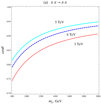
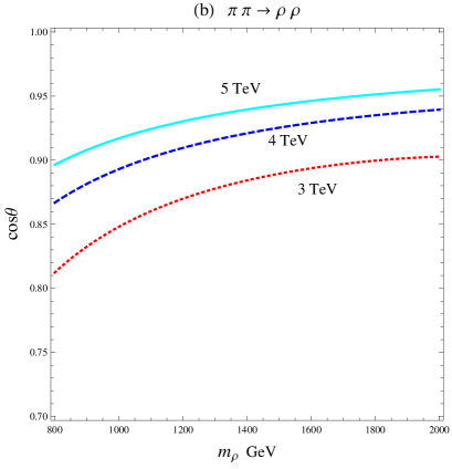
Figure 1: Parameter-space region where the unitarity bound $|$Re$a^{0}_{0}(s)^{(\pi\pi)}|\leq\frac{1}{2}$ is violated at energies $s\leq\Lambda^{2}$, for $\Lambda=3.0$ TeV (red dotted line), $\Lambda=4.0$ TeV (blue dashed line) and $\Lambda=5.0$ TeV (cyan solid line), with $g_{\rho}=2.0$, i.e. only the regions above the lines are permitted by perturbative unitary. The left panel is for the pion elastic scattering and the right panel is for the pion inelastic scattering.

3.2 $\pi\pi\to hh$ scattering

For the inelastic scattering: $A({\pi^{a}}{\pi^{b}}\to{h}{h})=A{(s,t,u)^{(hh)}}{\delta^{ab}}$. The isospin structure is quite simple in this process and it gets a contribution from the contact interaction, along with $\pi$, $\rho_{L}$, and $\rho_{R}$ exchanged $t$ and $u$ channels. The full prediction is:

$$A(s,t,u)^{(hh)}=-\frac{b}{v^{2}}s-\frac{a^{2}}{v^{2}}\left[{\frac{\left({t-m_{h}^{2}}\right)^{2}}{t}+\frac{\left({u-m_{h}^{2}}\right)^{2}}{u}}\right]+\frac{a_{\rho L}^{2}+a_{\rho R}^{2}}{4f^{2}}(-3s+2m_{h}^{2})$$

$$\qquad-~{}\frac{a_{\rho L}^{2}}{4f^{2}}m_{\rho L}^{2}\left(\frac{s-u}{t-m_{\rho L}^{2}}+\frac{s-t}{u-m_{\rho L}^{2}}\right)-\frac{a_{\rho L}^{2}}{4f^{2}}m_{h}^{4}\left(\frac{1}{t-m_{\rho L}^{2}}+\frac{1}{u-m_{\rho L}^{2}}\right)$$

$$\qquad-~{}\frac{a_{\rho R}^{2}}{4f^{2}}m_{\rho R}^{2}\left(\frac{s-u}{t-m_{\rho R}^{2}}+\frac{s-t}{u-m_{\rho R}^{2}}\right)-\frac{a_{\rho R}^{2}}{4f^{2}}m_{h}^{4}\left(\frac{1}{t-m_{\rho R}^{2}}+\frac{1}{u-m_{\rho R}^{2}}\right)$$ (21)

One may then perform a PW projection similar to that in Eq. (16) but with the effect of Higgs mass included in $\cos\alpha=2(t-m_{h}^{2}+s/2)/(s\beta_{h}(s))$ and the phase-space factor $\beta_{h}(s)=\sqrt{1-4m_{h}^{2}/s}$. In the light Higgs limit $m_{h}^{2}\ll|s|$ one gets

$$a^{0}_{0}(s)^{(hh)} = \frac{\displaystyle 1}{\displaystyle 2}\,a^{0}_{0}(s)^{(\pi\pi)}\,.$$ (22)

Here we made use of $a=\cos\theta$ and $b=\cos 2\theta$. With the existence of $SO(5)$ global symmetry, we expect to get the same expectation as in $\pi\pi\to\pi\pi$ when we demand the ${\cal O}(s)$ term to exactly cancel out at high energies. Nonetheless, due to the extra factor $\frac{1}{2}$, the violation of our “unitarity bound” by the linear $s$ divergence and the residual $\ln(s)$ high energy divergence occurs later.

3.3 $\pi\pi\to\rho\rho$ scattering

Now we come to consider the inelastic scattering $\pi^{a}\pi^{b}\to\rho_{L}^{c}\rho_{L}^{d}$, where the longitudinal component of the vector meson is parametrized as $\epsilon_{L}(k)=\bigg{(}\frac{\sqrt{s}}{2}\frac{\beta_{\rho}}{m_{\rho}},\frac{\sqrt{s}}{2m_{\rho}}\vec{n}_{k}\bigg{)}$ with $\beta_{\rho}=\sqrt{1-4m_{\rho}^{2}/s}$. As the Higgs is realized as one pNGB, the Higgs coupling $\frac{c_{\rho}}{f^{2}}m_{\rho}^{2}vh\rho_{\mu}^{a}\rho_{\mu}^{a}$ comes from the mass term of the vector meson and the parameter $c_{\rho}$ is suppressed by $g_{0}^{2}/g_{\rho}^{2}$. The isospin decomposition is similar to the elastic one but with two form factors. For $A(s,t,u)$ three diagrams contribute: the $s$ channel $h^{0}$ exchanged diagram, $t$ channel and $u$ channel $\pi$ exchanged diagrams; whereas for $B(s,t,u)$, there is one $\rho_{\mu}$ mediated $s$ channel diagram, one $\pi$ mediated $u$ channel diagram, and one $h^{0}$ mediated $t$ channel diagram:

$$A({\pi^{a}}{\pi^{b}}\to{\rho_{L}^{c}}{\rho_{L}^{d}})=A(s,t,u)^{(\rho\rho)}{\delta^{ab}}{\delta^{cd}}+B(s,t,u)^{(\rho\rho)}{\delta^{ac}}{\delta^{bd}}+B(s,u,t)^{(\rho\rho)}{\delta^{ad}}{\delta^{bc}},$$ (23)

$$A(s,t,u) = \frac{ac_{\rho}}{f^{2}}\frac{s(s-2m_{\rho}^{2})}{s-m_{h}^{2}}+\frac{a_{\rho}^{2}}{4f^{2}\beta_{\rho}^{2}}\frac{1}{u}\left(\frac{s}{2}\left(\beta_{\rho}^{2}+1\right)+t-m_{\rho}^{2}\right)^{2}$$ (24)

$$+ \frac{a_{\rho}^{2}}{4f^{2}\beta_{\rho}^{2}}\frac{1}{t}\left(\frac{s}{2}\left(\beta_{\rho}^{2}-1\right)-t+m_{\rho}^{2}\right)^{2}~{},$$

$$B(s,t,u) = \frac{1}{4f^{2}}\frac{(s+2m_{\rho}^{2})(t-u)}{(s-m_{\rho}^{2})}+\frac{a_{\rho}^{2}}{4f^{2}\beta_{\rho}^{2}}\frac{1}{u}\left(\frac{s}{2}\left(\beta_{\rho}^{2}+1\right)+t-m_{\rho}^{2}\right)^{2}$$ (25)

$$+ \frac{a_{\rho}^{2}}{4f^{2}\beta_{\rho}^{2}}\frac{1}{(t-m_{h}^{2})}\left(\frac{s}{2}\left(\beta_{\rho}^{2}-1\right)-t+m_{\rho}^{2}\right)^{2}~{}.$$

Since the vector resonance is introduced to restore the perturbative unitary, it is usually demanded that the cutoff scale satisfying $2m_{\rho}<\Lambda<4\pi f$. When the threshold effect of the final states could be ignored, i.e. $m_{\rho}\ll\Lambda$, there are only linear growing $s$ term and constant term in the partial wave transformation. But as the mass $m_{\rho}$ is comparable with $\Lambda$, logarithmic terms also appear:

$$a^{0}_{0}(s)^{(\rho\rho)}=\frac{\displaystyle\left(24ac_{\rho}\beta_{\rho}^{3}+10a_{\rho}^{2}\left(1-2\beta_{\rho}^{2}\right)\beta_{\rho}+5a_{\rho}^{2}\left(1-\beta_{\rho}^{2}\right)^{2}\log\left(\frac{(1-\beta_{\rho})s-2m_{\rho}^{2}}{(1+\beta_{\rho})s-2m_{\rho}^{2}}\right)\right)s}{\displaystyle 256\pi f^{2}\beta_{\rho}^{3}}$$

$$\quad-\frac{\displaystyle\left(\left(12ac_{\rho}\beta_{\rho}^{2}+5a_{\rho}^{2}\right)\beta_{\rho}+5a_{\rho}^{2}\left(\left(1-\beta_{\rho}^{2}\right)-\frac{m_{\rho}^{2}}{s}\right)\log\left(\frac{(1-\beta_{\rho})s-2m_{\rho}^{2}}{(1+\beta_{\rho})s-2m_{\rho}^{2}}\right)\right)m_{\rho}^{2}}{\displaystyle 64\pi f^{2}\beta_{\rho}^{3}}$$ (26)

In the limit $m_{h},m_{\rho}\ll\Lambda$, the partial wave displays a linear growing pattern: $a^{0}_{0}(s)^{(\rho\rho)}\simeq\frac{\displaystyle s}{\displaystyle 128\pi f^{2}}{\bigg{(}12ac_{\rho}-5a_{\rho}^{2}\bigg{)}}$, which pushes the partial wave to grow quickly after the two mesons threshold is reached, and this process provides a complementary constraint for the parameter space. In Fig. 1 (b), with the $c_{\rho}$ term ignored, we show that the unitary bound actually imposes a more stringent constraint on the parameter space, that is it requires one larger value of global symmetry breaking scale $f$ (i.e. $\cos\theta$ needs to be more close to 1) for the same value of $m_{\rho}$ and $\Lambda$ as compared with the elastic scattering.

4 Higgs to diphotons from $\rho$ mesons

In this section, we discuss the resonance effects on the Higgs sector. The gauge bosons couple to the vector resonances via the mass terms described in Eq.(6-7), since it is the combination of $(g_{\rho}\tilde{\rho}_{\mu}^{L,R}-E_{\mu}^{L,R})$ that transforms homogeneously under the symmetry group of $SO(4)$. Due to the mixing between the gauge eigenstates of $\tilde{\rho}_{L\mu}^{a}$, $\tilde{W}_{\mu}^{a}$, $\tilde{\rho}_{R\mu}^{3}$ and $\tilde{B}_{\mu}$, the exact gauge bosons in the effective theory gain the property of partial compositeness. At the leading order of $\xi=v^{2}/f^{2}=(1-\cos^{2}\theta)$, the mass terms are simplified as:

$$\mathcal{L}_{\rho}^{m} = \frac{m_{\rho}^{2}}{2g_{\rho}^{2}}\left(g_{\rho}\tilde{\rho}_{L\mu}^{a}-g_{0}\tilde{W}_{\mu}^{a}\right)^{2}+\frac{m_{\rho}^{2}}{2g_{\rho}^{2}}\left(g_{\rho}\tilde{\rho}_{R\mu}^{3}-g_{0}^{\prime}\tilde{B}_{\mu}\right)^{2}$$ (27)

such that the gauge couplings for $SU(2)_{L}\times U(1)_{Y}$ in the standard model are determined by the relations of:

$$g_{2}^{2}=\frac{g_{0}^{2}g_{\rho}^{2}}{{g_{0}^{2}+g_{\rho}^{2}}}~{},\quad g_{1}^{2}=\frac{{g_{0}^{\prime 2}g_{\rho}^{2}}}{{g_{0}^{\prime 2}+g_{\rho}^{2}}}$$ (28)

In the following analysis, we will take the same benchmark point $g_{\rho}=2.0$ as in the last section, therefore $g_{0}$ and $g_{0}^{\prime}$ are fixed in order to reproduce the SM model couplings $g_{1}$ and $g_{2}$ at the electroweak scale. Including higher order expansion of the Higgs fields, the mixing would be further modified, as indicated by the following derivation. In the unitary gauge, all the pion fields are eaten and the Goldstone boson in the fourth direction is the Higgs field, i.e. $\pi^{4}\simeq h^{0}$. There is one interaction term in the form of $(h^{0})^{2}(g_{0}\tilde{W}_{\mu}^{a}-g_{0}^{\prime}\tilde{B}_{\mu}\delta^{a3})$ embedded in the connection $E_{\mu}$’s explicit expression :

$$E_{\mu} = \left({g_{0}}\tilde{W}_{\mu}^{a}T_{L}^{a}+g_{0}^{\prime}\tilde{B}_{\mu}T_{R}^{3}\right)+\frac{1}{f^{2}}\left[h^{0}~{}T^{\hat{4}},[{g_{0}\tilde{W}_{\mu}^{a}}T_{L}^{a}+g_{0}^{\prime}\tilde{B}_{\mu}T_{R}^{3},h^{0}~{}T^{\hat{4}}]\right]+\cdots$$ (29)

$$= \left(g_{0}\tilde{W}_{\mu}^{a}T_{L}^{a}+g_{0}^{\prime}\tilde{B}_{\mu}T_{R}^{3}\right)-\frac{(h^{0})^{2}}{4f^{2}}(g_{0}\tilde{W}_{\mu}^{a}-g_{0}^{\prime}\tilde{B}_{\mu}\delta^{a3})(T_{L}^{a}-T_{R}^{a})+\cdots$$

With the EW symmetry breaking, the second term in the above equation gives rise to one new interaction term between the Higgs fields and gauge bosons.

Substituting both $(h^{0})^{2}$ by their VEVs would modify the mixing among the gauge bosons and vector mesons. Assuming the charged $W_{\mu}^{\pm}$ gauge bosons are zero modes, we will retain the correction occurring at the linear order of $\xi$ but are justified to ignore corrections at the order of $m_{W}^{2}/m_{\rho}^{2}$. The full rotation for the charged gauge bosons is:

$$\tilde{W}_{\mu}^{\pm} = \frac{g_{\rho}W_{\mu}^{\pm}+g_{0}\rho_{L\mu}^{\pm}}{(g_{\rho}^{2}+g_{0}^{2})^{1/2}}+\frac{\xi g_{\rho}g_{0}(g_{0}W_{\mu}^{\pm}-g_{\rho}\rho_{L\mu}^{\pm})}{4(g_{\rho}^{2}+g_{0}^{2})^{3/2}}$$ (30)

$$\tilde{\rho}_{L\mu}^{\pm} = \frac{{g_{0}}{W_{\mu}^{\pm}}-{g_{\rho}}\rho_{L\mu}^{\pm}}{(g_{\rho}^{2}+g_{0}^{2})^{1/2}}-\frac{\xi g_{\rho}g_{0}(g_{\rho}W_{\mu}^{\pm}+g_{0}\rho_{L\mu}^{\pm})}{4(g_{\rho}^{2}+g_{0}^{2})^{3/2}}-\frac{\xi}{4}\rho_{R\mu}^{\pm}$$ (31)

$$\tilde{\rho}_{R\mu}^{\pm} = \rho_{R\mu}^{\pm}+\frac{\xi(g_{0}W_{\mu}^{\pm}-g_{\rho}\rho_{L\mu}^{\pm})}{4(g_{\rho}^{2}+g_{0}^{2})^{1/2}}$$ (32)

where $\rho_{L}^{\pm}$ and $\rho_{R}^{\pm}$ are mass eigenstates with corresponding masses of $m_{\rho_{L}}^{2}=g_{\rho}^{2}a_{\rho}^{2}f^{2}$ and $m_{\rho_{R}}^{2}=(g_{\rho}^{2}+g_{0}^{2}(1+\xi/4))a_{\rho}^{2}f^{2}$. The neutral gauge bosons mixing pattern is distinct from the charged ones as indicated by the $E_{\mu}$ expression [see Eq.(29)]. The eigenstates for the three massive neutral states are rather complicated. However it is easy to project out the exact zero mode, i.e. the photon, which is the combination of the four neutral gauge eigenstates $\tilde{W}_{\mu}^{3}$, $\tilde{B}_{\mu}$, and $\tilde{\rho}_{L\mu}^{3}$ , $\tilde{\rho}_{R\mu}^{3}$:

$${A_{\mu}} = \frac{{g_{0}^{\prime}}{g_{0}}{{\tilde{\rho}}_{L\mu}}+{g_{0}^{\prime}}{g_{0}}{{\tilde{\rho}}_{R\mu}}+{g_{\rho}}({g_{0}^{\prime}}{{\tilde{W}}_{\mu}^{3}}+{g_{0}}{{\tilde{B}}_{\mu}})}{\sqrt{g_{\rho}^{2}(g_{0}^{\prime 2}+g_{0}^{2})+2g_{0}^{\prime 2}g_{0}^{2}}}$$ (33)

and for completeness the Weinberg mixing angle and the electromagnetic coupling are given as:

$$c_{w}^{2}=\frac{g_{0}^{2}(g_{0}^{\prime 2}+g_{\rho}^{2})}{2g_{0}^{2}g_{0}^{\prime 2}+\left(g_{0}^{\prime 2}+g_{0}^{2}\right)g_{\rho}^{2}}\approx\frac{g_{0}^{2}}{g_{0}^{\prime 2}+g_{0}^{2}}$$ (34)

$$s_{w}^{2}=\frac{g_{0}^{\prime 2}(g_{0}^{2}+g_{\rho}^{2})}{2g_{0}^{2}g_{0}^{\prime 2}+\left(g_{0}^{\prime 2}+g_{0}^{2}\right)g_{\rho}^{2}}\approx\frac{g_{0}^{\prime 2}}{g_{0}^{\prime 2}+g_{0}^{2}}$$ (35)

$$e=\frac{g_{0}g_{0}^{\prime}g_{\rho}}{\sqrt{2g_{0}^{2}g_{0}^{\prime 2}+\left(g_{0}^{\prime 2}+g_{0}^{2}\right)g_{\rho}^{2}}}\approx\frac{g_{0}g_{0}^{\prime}}{g_{0}^{2}+g_{0}^{\prime 2}}$$ (36)

which are consistent with the SM formulas as we abandon the corrections at the order of $g_{0}^{\prime}/g_{\rho}$ and $g_{0}/g_{\rho}$. We prefer to conduct the calculation with the mass eigenstate since the trilinear gauge interaction with one photon and the quartic gauge interaction with two photons are diagonal in that basis.

On the other hand, with only one $h^{0}$ gain VEV in Eq. (29) and the mixing mass term gives us the following Lagrangian for $H$-$\tilde{\rho}$-$\tilde{W}$and $H$-$\tilde{\rho}$-$\tilde{B}$ interactions:

$$\mathcal{L}_{\rm{mix}}=\frac{m_{\rho}^{2}\xi}{2g_{\rho}v}h^{0}\tilde{\rho}_{L\mu}^{a}(g_{0}\tilde{W}_{\mu}^{a}-g_{0}^{\prime}\tilde{B}_{\mu}\delta^{a3})-\frac{m_{\rho}^{2}\xi}{2g_{\rho}v}h^{0}\tilde{\rho}_{R\mu}^{a}(g_{0}\tilde{W}_{\mu}^{a}-g_{0}^{\prime}\tilde{B}_{\mu}\delta^{a3})$$ (37)

Adapting it in terms of the mass eigenstates, we find positive shifts for the $h^{0}W_{\mu}^{+}W_{\mu}^{-}$ and $h^{0}Z_{\mu}^{0}Z_{\mu}^{0}$ vertices and a negative shift for the $h^{0}\rho_{L\mu}^{+}\rho_{L\mu}^{-}$ at the leading order of $\xi=v^{2}/f^{2}$. It is convenient to parametrize the Higgs interactions with the gauge bosons adopting the effective theory approach:

$$\mathcal{L}_{eff} = a_{W}\frac{2m_{W}^{2}}{v}h^{0}W_{\mu}^{+}W_{\mu}^{-}+a_{Z}\frac{m_{Z}^{2}}{v}h^{0}Z_{\mu}Z_{\mu}+c_{\rho}\frac{2m_{\rho}^{2}}{v}h^{0}\rho_{L\mu}^{+}\rho_{L\mu}^{-}$$ (38)

$$+ c_{\rho_{R}W}\frac{m_{\rho}^{2}}{v}h^{0}\left(W_{\mu}^{+}\rho_{R\mu}^{-}+W_{\mu}^{-}\rho_{R\mu}^{+}\right)+c_{\rho_{L}\rho_{R}}\frac{m_{\rho}^{2}}{v}h^{0}\left(\rho_{L\mu}^{+}\rho_{R\mu}^{-}+\rho_{L\mu}^{-}\rho_{R\mu}^{+}\right)$$

$$+ {c_{f}}\left(\frac{m_{f}}{v}\bar{f}f\right)h_{0}+c_{\gamma}\frac{\alpha}{8\pi v}h^{0}A^{\mu\nu}A_{\mu\nu}+c_{Z\gamma}\frac{\alpha}{4\pi v}h^{0}Z^{\mu\nu}A_{\mu\nu}$$

$$a_{W} = \left(\frac{g_{\rho}^{2}}{g_{0}^{2}+g_{\rho}^{2}}+\frac{g_{0}^{2}g_{\rho}^{2}\xi}{2(g_{0}^{2}+g_{\rho}^{2})^{2}}\right)\cos\theta+\frac{g_{0}^{2}\xi}{2(g_{0}^{2}+g_{\rho}^{2})}\frac{m_{\rho}^{2}}{m_{W}^{2}}$$ (39)

$$c_{\rho} = \left(\frac{g_{0}^{2}}{g_{0}^{2}+g_{\rho}^{2}}-\frac{g_{0}^{2}g_{\rho}^{2}\xi}{2(g_{0}^{2}+g_{\rho}^{2})^{2}}\right)\frac{m_{W}^{2}}{m_{\rho}^{2}}\cos\theta-\frac{g_{0}^{2}\xi}{2(g_{0}^{2}+g_{\rho}^{2})}$$ (40)

$$a_{Z} = \cos\theta+\frac{\left(g_{0}^{2}+g_{0}^{\prime 2}\right)m_{\rho}^{2}\xi}{2g_{\rho}^{2}m_{Z}^{2}}$$ (41)

where the third terms in $a_{W}$ and $c_{\rho}$ and the second term in $a_{Z}$ come from the mass mixing terms $h^{0}\tilde{\rho}_{L}^{a}(g_{0}\tilde{W}^{a}-g_{0}^{\prime}\tilde{B}\delta^{a3})$ and $h^{0}\tilde{\rho}_{R}^{a}(g_{0}\tilde{W}^{a}-g_{0}^{\prime}\tilde{B}\delta^{a3})$, and the $c_{\gamma}$ term is originated through the loop contribution of heavy charged particles. Notice that only diagonal vertices are relevant to the branching ratio of Higgs decay into diphoton whereas there are additional nondiagonal Higgs vertices along with nondiagonal trilinear and quartic gauge interactions which would contribute to $h^{0}\to Z\gamma$. The latter process is correlated to $h^{0}\to\gamma\gamma$ due to the electroweak symmetry. The corrections to $c_{\gamma}$ come from the vector meson and its mixing with $W$, $Z$ gauge bosons:

$$c_{\gamma} = {c_{t}}{N_{c}}(2/3)^{2}F_{1/2}(4m_{t}^{2}/m_{h}^{2})+a_{W}{F_{1}}(4m_{W}^{2}/m_{h}^{2})+c_{\rho}{F_{1}}(4m_{\rho}^{2}/m_{h}^{2})$$ (42)

$$F_{1/2}(x)=-2x\left(1+(1-x)\arcsin^{2}(x^{-1/2})\right)$$ (43)

$$F_{1}(x)=2+3x+3x(2-x){\arcsin^{2}(x^{-1/2})}$$ (44)

with $x_{i}=4m_{i}^{2}/m_{W}^{2}$. For the large mass limit of $\rho$ mesons and top quark mass, the asymptotic values for those form functions are: $F_{1}(x)\approx 7$ and $F_{1/2}(x)\approx-4/3$ .

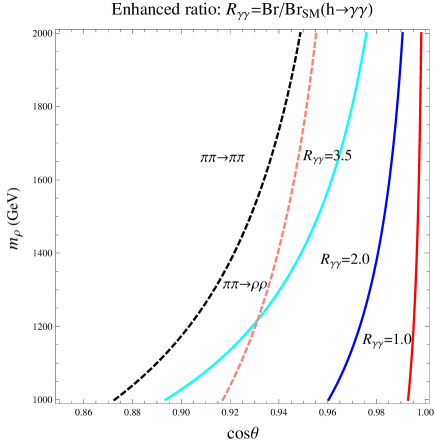
Figure 2: Contour plot for the $R_{\gamma\gamma}$ in the gluon fusion channel assuming $c_{t}=1$. The black dashed line is the unitary bound for the elastic pion scattering $\pi\pi\to\pi\pi$ and the orange dashed line is the unitary bound for the inelastic scattering $\pi\pi\to\rho\rho$ with $\Lambda=5$ TeV. The region approaching the $\cos\theta=1$ direction is permitted.

With the knowledge of those couplings, the partial width for Higgs to diphoton in the composite Higgs model with respect to its prediction in the SM and the respective ratios for the other two bosons channels are fixed to be:

$$\Gamma/\Gamma(H\to\gamma\gamma)^{sm}=\frac{c_{\gamma}^{2}}{c_{\gamma,sm}^{2}},\Gamma/\Gamma(H\to WW^{*})^{sm}=\frac{a_{W}^{2}}{a_{W,sm}^{2}},\Gamma/\Gamma(H\to ZZ^{*})^{sm}=\frac{a_{Z}^{2}}{a_{Z,sm}^{2}}$$ (45)

However at the LHC, only the product of $\sigma\times Br(h\to VV^{\prime})$ is measurable.The variable, which indicates the deviation of composite Higgs models from the standard model, is the so-called $R$ parameter [10], i.e. the observing signal events divided by its corresponding SM expectation. For the diphoton process, the $R_{\gamma\gamma}$ is defined as:

$$R_{\gamma\gamma}=\frac{\sigma\left(pp\to h^{0}X\right)}{\sigma_{sm}\left(pp\to h^{0}X\right)}\times\frac{Br(h^{0}\to\gamma\gamma)}{Br_{sm}(h^{0}\to\gamma\gamma)}$$ (46)

where $\sigma$ is the production cross section for the Higgs boson and $X$ denotes any particle associatively produced with the Higgs boson. At the available energy scale, the main production channels for the Higgs bosons are gluon fusions $gg\to h^{0}$ and vector boson fusions $q\bar{q}\to h^{0}jj$. The modified cross sections for those two processes are [11]:

$$\frac{\sigma}{\sigma_{sm}}(gg\to h^{0})=c_{t}^{2}~{},\quad\frac{\sigma}{\sigma_{sm}}(gg\to h^{0}jj)=\frac{a_{W}^{2}\sigma_{sm}^{W}+a_{Z}^{2}\sigma_{sm}^{Z}}{\sigma_{sm}^{W}+\sigma_{sm}^{Z}}.$$ (47)

For simplicity, in this paper we are going to assume that all the fermion couplings are the same as they are in the SM , i.e. $c_{f}=1$, with the consequence that the top quark induced gluon fusion cross section is the same as in the SM. The observing ratios for the diphoton process could be expressed in a more convenient form:

$$R_{\gamma\gamma}=\frac{\sigma/\sigma_{sm}\cdot|c_{\gamma}/c_{\gamma}^{sm}|^{2}}{a_{W}^{2}Br_{sm}^{(WW^{*})}+a_{Z}^{2}Br_{sm}^{(ZZ^{*})}+|c_{\gamma}/c_{\gamma}^{sm}|^{2}Br_{sm}^{(\gamma\gamma)}+\cdots}$$ (48)

The $R_{\gamma\gamma}$ dependence on the $(\cos\theta,m_{\rho})$ for the gluon fusion channel is plotted in Fig. 2. We put the unitary bound on that plot by requiring that the perturbative unitary is violated at $\Lambda=5$ TeV. As we can see, if we demand that the composite Higgs model prediction does not give a significant deviation from the LHC measurement, the perturbative unitary is a very loose requirement for the allowed parameter space. To achieve a diphoton enhancement rate not larger than a factor of 1.5, we roughly need $\cos\theta>0.97$ and $m_{\rho}>1.0$ TeV. The $R_{\gamma\gamma}$ in the vector boson fusion process is similar, but with $a_{W},a_{Z}>1$, a larger diphoton enhancement rate is encountered in this channel.

Adding new fermion resonances to the composite model would be quite interesting since, under certain circumstance, it possibly enhances the production cross section of Higgs bosons but at the same time it reduces the decay branching ratio into diphotons. The balanced effect might depend on the specific model details. Furthermore, those composite fermions are introduced into the model as vector-like quarks, thus their mixing with the SM quarks would inevitably modify the $W$-$t$-$b$ and $Z$-$b$-$b$ vertices and possibly give a notable contribution to the oblique parameters [12]. Detailed studies need to be devoted to explore the influence of the third generation composite quarks on the Higgs sector [13, 14, 15].

5 Conclusion

In summary, for a light composite Higgs boson which is realized as one pNGB from a strong interacting sector, $\pi\pi$ scatterings put some mild constraint on the $(\cos\theta,m_{\rho})$ parameter space. We conduct a careful analysis for both the elastic and inelastic pion scatterings and the deviation of the Higgs to gauge couplings from the standard model occurring at the order of $v^{2}/f^{2}$ is allowed as we reduce $m_{\rho}$, the mass of composite meson field. The nonlinear realization enriches the Higgs interaction with SM gauge bosons. It is noticed that in the minimal $SO(5)/SO(4)$ coset model, with the presence of vector mesons in the fundamental representation of $SO(4)$, a new interaction originating from the strong interacting sector may shift the Higgs couplings $a_{W}$ and $a_{Z}$ in the positive direction due to the partial compositeness of $W$ and $Z$ gauge bosons after electroweak symmetry breaking. Therefore it is easy for us to accommodate an enhancement of diphoton rate which is observed at the LHC. It is believed that through extending the model structure (with effects on Higgs productions and decays) and fine tuning the parameter space, the light composite Higgs probably could fit the experimental measurements much better than the standard model.

Note: It is interesting to observe that there is nondiagonal contribution to Higgs coupling to $Z$ and photon. The calculation for this form factor is put in the appendix.

Appendix A non-diagonal gauge boson contribution to $H$-$Z$-$\gamma$

In this appendix, we are going to show that including non-diagonal couplings exclusively results in a gauge-inviarant contribution for the form factor $c_{Z\gamma}$. Similar nondiagonal ccontribution from charginos in the MSSM is calculated in a reference [16].

Figure 3: (a) triangle feyndiagram with one vector resonance, (b) triangle feyndiagram with two vector resonances , (c) quartic feyndiagram with one vector resonance.

Assuming there is one non-diagonal Higgs-gauge coupling $c_{\rho_{R}W}\frac{\displaystyle m_{\rho}^{2}}{\displaystyle v}\left(h^{0}\rho_{R,\mu}^{+}W_{\mu}^{-}+h.c.\right)$ and we can express some generic non-diagonal trilinear and quartic gauge self couplings in the following way:

$$\mathcal{L}_{Z\rho_{R}W} = (-i\,e\,\cot\theta_{w})\,c_{Z\rho_{R}W}\bigg{(}\partial_{\mu}Z_{\nu}\rho_{R,\mu}^{+}W_{\nu}^{-}+\partial_{\mu}\rho_{R,\nu}^{+}W_{\mu}^{-}Z_{\nu}+\partial_{\mu}W_{\nu}^{-}Z_{\mu}\rho_{R,\nu}^{+}$$ (49)

$$+ \partial_{\mu}Z_{\nu}\rho_{R,\nu}^{-}W_{\mu}^{+}+\partial_{\mu}\rho_{R,\nu}^{-}W_{\nu}^{+}Z_{\mu}+\partial_{\mu}W_{\nu}^{+}Z_{\nu}\rho_{R,\mu}^{-}-\left(\mu\leftrightarrow\nu\right)\bigg{)}$$

$$\mathcal{L}_{AZ\rho_{R}W} = (e^{2}\,\cot\theta_{w})\,c_{Z\rho_{R}W}\bigg{(}2~{}Z_{\mu}A_{\mu}\rho^{+}_{R,\nu}W^{-}_{\nu}-Z_{\mu}A_{\nu}\rho^{+}_{R,\mu}W^{-}_{\nu}-Z_{\nu}A_{\mu}\rho^{+}_{R,\mu}W^{-}_{\nu}$$ (50)

$$+ 2~{}Z_{\mu}A_{\mu}\rho^{-}_{R,\nu}W^{+}_{\nu}-Z_{\mu}A_{\nu}\rho^{-}_{R,\nu}W^{+}_{\mu}-Z_{\nu}A_{\mu}\rho^{-}_{R,\nu}W^{+}_{\mu}\bigg{)}$$

The amplitude for Higgs decay into $Z$ and photon is adding up the three diagrams illustrated in Fig.[3] and it is necessary to times a factor of two to account for the crossing symmetry. As we put all the external particles to be on shell, the amplitude can be organized into a gauge invariant form:

$$M({h^{0}}\to Z\gamma)=2\cdot\left(M^{(a)}+M^{(b)}+M^{(c)}\right)$$ (51)

$$= \frac{-i\,e^{2}}{8\pi^{2}v}\left(2\,\,c_{\rho_{R}W}\,c_{Z\rho_{R}W}\right)\,c_{Z\gamma}^{(1)}\,\left({{g^{\mu\nu}}{k_{1}}\cdot{k_{2}}-k_{1}^{\mu}k_{2}^{\nu}}\right)\,\varepsilon_{\mu}^{*}({k_{1}})\varepsilon_{\nu}^{*}({k_{2}})$$

It is convenient to express the form factor $c_{Z\gamma}^{(1)}$ in terms of one-loop three-point scalar and vector functions, i.e. $C_{0}(m_{h}^{2},m_{Z}^{2},0,m_{2}^{2},m_{1}^{2},m_{2}^{2})$ and $C_{2}(m_{h}^{2},m_{Z}^{2},0,m_{2}^{2},m_{1}^{2},m_{2}^{2})$ defined in [17], with two different masses circulating in the loop.

$$c_{Z\gamma}^{(1)} = \cot\theta_{w}\cdot\frac{m_{\rho}^{2}}{m_{W}^{2}}\cdot\bigg{[}\left(\left({\frac{m_{h}^{2}}{m_{\rho}^{2}}+\frac{m_{W}^{2}}{m_{\rho}^{2}}+1}\right)\left(m_{Z}^{2}-m_{\rho}^{2}-m_{W}^{2}\right)-8m_{W}^{2}\right)$$ (52)

$$\cdot \bigg{(}C_{2}\left(m_{h}^{2},m_{Z}^{2},0,m_{W}^{2},m_{\rho}^{2},m_{W}^{2}\right)+C_{2}\left(m_{h}^{2},m_{Z}^{2},0,m_{\rho}^{2},m_{W}^{2},m_{\rho}^{2}\right)\bigg{)}$$

$$+ 2\left(\frac{m_{W}^{2}}{m_{\rho}^{2}}\left(m_{Z}^{2}-m_{W}^{2}-3m_{\rho}^{2}\right)\right)\cdot C_{0}\left(m_{h}^{2},m_{Z}^{2},0,m_{W}^{2},m_{\rho}^{2},m_{W}^{2}\right)$$

$$+ 2\left(m_{Z}^{2}-3m_{W}^{2}-m_{\rho}^{2}\right)\cdot C_{0}\left(m_{h}^{2},m_{Z}^{2},0,m_{\rho}^{2},m_{W}^{2},m_{\rho}^{2}\right)\bigg{]}$$

where the special combination of vector functions in the large bracket can be recasted into Passarino-Veltman functions $B_{0}$ and $C_{0}$:

$$C_{2}\left(m_{h}^{2},m_{Z}^{2},0,m_{W}^{2},m_{\rho}^{2},m_{W}^{2}\right)+C_{2}\left(m_{h}^{2},m_{Z}^{2},0,m_{\rho}^{2},m_{W}^{2},m_{\rho}^{2}\right)$$ (53)

$$= \frac{m_{Z}^{2}}{\left({m_{Z}^{2}-m_{h}^{2}}\right)^{2}}\bigg{(}B_{0}\left({m_{Z}^{2},m_{\rho}^{2},m_{W}^{2}}\right)-B_{0}\left({m_{h}^{2},m_{\rho}^{2},m_{W}^{2}}\right)\bigg{)}$$

$$+ \frac{1}{\left({m_{Z}^{2}-m_{h}^{2}}\right)}+\frac{m_{W}^{2}}{\left(m_{Z}^{2}-m_{h}^{2}\right)}C_{0}\left(m_{h}^{2},m_{Z}^{2},0,m_{W}^{2},m_{\rho}^{2},m_{W}^{2}\right)$$

$$+ \frac{m_{\rho}^{2}}{\left(m_{Z}^{2}-m_{h}^{2}\right)}C_{0}\left(m_{h}^{2},m_{Z}^{2},0,m_{\rho}^{2},m_{W}^{2},m_{\rho}^{2}\right)$$

It should be noticed that in the limit of $m_{\rho}=m_{W}$, our new form factor $c_{Z\gamma}^{(1)}$ will reduce exactly to the $W$ gauge bosons mediated SM contribution[18].

References

- [1] R. Contino, Y. Nomura and A. Pomarol, Nucl. Phys. B 671, 148 (2003) [hep-ph/0306259]; K. Agashe, R. Contino and A. Pomarol, Nucl. Phys. B 719, 165 (2005) [hep-ph/0412089].
- [2] A. Falkowski and M. Perez-Victoria, Phys. Rev. D 79, 035005 (2009) [arXiv:0810.4940 [hep-ph]]; H. Cai, H. -C. Cheng, A. D. Medina and J. Terning, Phys. Rev. D 80, 115009 (2009) [arXiv:0910.3925 [hep-ph]]; H. Cai, H. -C. Cheng, A. D. Medina and J. Terning, Phys. Rev. D 85, 015019 (2012) [arXiv:1108.3574 [hep-ph]].
- [3] C. Anastasiou, E. Furlan and J. Santiago, Phys. Rev. D 79, 075003 (2009) arXiv:0901.2117 [hep-ph]; G. Panico and A. Wulzer, JHEP 1109, 135 (2011) arXiv:1106.2719 [hep-ph]; S. De Curtis, M. Redi and A. Tesi, JHEP 1204, 042 (2012) arXiv:1110.1613 [hep-ph] .
- [4] G. Aad et al. [ATLAS Collaboration], Phys. Lett. B 716 (2012) 1 arXiv:1207.7214 [hep-ex]; S. Chatrchyan et al. [CMS Collaboration], Phys. Lett. B 716 (2012) 30 arXiv:1207.7235 [hep-ex].
- [5] S. R. Coleman, J. Wess and B. Zumino, Phys. Rev. 177, 2239 (1969); C. G. Callan, Jr., S. R. Coleman, J. Wess and B. Zumino, Phys. Rev. 177, 2247 (1969).
- [6] R. Contino, D. Marzocca, D. Pappadopulo and R. Rattazzi, JHEP 1110, 081 (2011) [arXiv:1109.1570 [hep-ph]].
- [7] D. Marzocca, M. Serone and J. Shu, JHEP 1208 (2012) 013 [arXiv:1205.0770 [hep-ph]].
- [8] B. Bellazzini, C. Csaki, J. Hubisz, J. Serra and J. Terning, JHEP 1211 (2012) 003 [arXiv:1205.4032 [hep-ph]].
- [9] Z.H. Guo, J.J. Sanz-Cillero and H.Q. Zheng, Phys.Lett. B661 (2008) 342-347 [arXiv:0710.2163 [hep-ph]];
- [10] D. Barducci, A. Belyaev, M. S. Brown, S. De Curtis, S. Moretti and G. M. Pruna, arXiv:1302.2371 [hep-ph].
- [11] G. Cacciapaglia, A. Deandrea, G. D. La Rochelle and J. -B. Flament, arXiv:1210.8120 [hep-ph].
- [12] L. Lavoura and J. P. Silva, Phys. Rev. D 47 (1993) 2046; H. Cai, JHEP 1302, 104 (2013) arXiv:1210.5200 [hep-ph].
- [13] A. Falkowski, Phys. Rev. D 77, 055018 (2008) [arXiv:0711.0828 [hep-ph]] ;
- [14] J. Kearney, A. Pierce and N. Weiner, Phys. Rev. D 86, 113005 (2012) arXiv:1207.7062 [hep-ph].
- [15] A. Carmona and F. Goertz, arXiv:1301.5856 [hep-ph].
- [16] A. Djouadi, V. Driesen, W. Hollik and A. Kraft, Eur. Phys. J. C 1, 163 (1998) [hep-ph/9701342].
- [17] G. ’t Hooft and M. J. G. Veltman, Nucl. Phys. B 153, 365 (1979); G. Passarino and M. J. G. Veltman, Nucl. Phys. B 160, 151 (1979); A. Denner, Fortsch. Phys. 41, 307 (1993) arXiv:0709.1075 [hep-ph]
- [18] F. Wilczek, Phys. Rev. Lett. 39 (1977) 1304; R.N. Cahn, M.S. Chanowitz and N. Fleishon, Phys. Lett. B82 (1979) 113; L. Bergstrom and G. Hulth, Nucl. Phys. B259 (1985) 137.