Cavity-QED of a leaky planar resonator coupled
to an atom and an input single-photon pulse

Abstract

In contrast to the free-space evolution of an atom governed by a multi-mode interaction with the surrounding electromagnetic vacuum, the evolution of a cavity-QED system can be characterized by just three parameters, (i) atom-cavity coupling strength $g$, (ii) cavity relaxation rate $\kappa$, and (iii) atomic decay rate into the non-cavity modes $\gamma$. In the case of an atom inserted into a planar resonator with an input beam coupled from the outside, it has been shown by Koshino [Phys. Rev. A 73, 053814 (2006)] that these three parameters are determined not only by the atom and cavity characteristics, but also by the spatial distribution of the input pulse. By an ab-initio treatment, we generalize the framework of Koshino and determine the cavity-QED parameters of a coupled system of atom, planar (leaky) resonator, and input single-photon pulse as functions of the lateral profile of the pulse and the length of resonator. We confirm that the atomic decay rate can be suppressed by tailoring appropriately the lateral profile of the pulse. Such an active suppression of atomic decay opens an attractive route towards an efficient quantum memory for long-term storage of an atomic qubit inside a planar resonator.

I Introduction

Cavity quantum electrodynamics (cavity-QED) is a research field that studies electromagnetic fields in confined spaces and radiative properties of atoms in such fields. Experimentally, the simplest example of such a system is a single atom interacting with a single mode of a high-finesse resonator rpp69 . This system bears an excellent framework for quantum communication and information processing, in which atoms and photons are interpreted as bits of quantum information and their mutual interaction provides a controllable entanglement mechanism rmp79 .

Remarkably, the evolution of a cavity-QED system can be well characterized by just three parameters: (i) atom-cavity coupling strength $g$, (ii) cavity relaxation rate $\kappa$, and (iii) atomic decay rate into the non-cavity modes $\gamma$. The cavity-QED effects become manifest clearly when the atom-cavity coupling $g$ is much larger than the atomic decay rate $\gamma$ and the cavity relaxation rate $\kappa$, at the same time. These two conditions define the (so-called) strong-coupling regime of atom-cavity interaction that ensures that the energy exchange between the constituents is reversible and develops faster than losses due to the cavity relaxation and the atomic decay. In the resonant regime, i.e., when the cavity resonant frequency matches the atomic transition frequency, the reversibility of energy exchange ensures that the coherent (unitary) part of atom-cavity evolution is governed by the Jaynes-Cummings Hamiltonian jc

$$H_{\text{JC}}=\hbar\,g\left(c\,\sigma^{\dagger}+c^{\dagger}\,\sigma\right)\,,$$ (1)

where $c$ and $c^{\dagger}$ denote the cavity mode annihilation and creation operators, while $\sigma$ and $\sigma^{\dagger}$ are the atomic lowering and raising operators, respectively. This Hamiltonian describes the interaction of a two-level atom with a single-mode light field that is confined inside the resonator.

During the last decades, single-mode resonators with typically spherical mirrors have been fabricated and utilized in various cavity-QED experiments. It was demonstrated that resonators with spherical mirrors can operate in the strong-coupling regime, such that the coherent part of the atom-cavity evolution is described by the Hamiltonian (1) prl93 . Although a planar Fabry-Perot resonator with a coupled atom is used to illustrate the main features of cavity-QED, there is an essential difference between the resonator with spherical mirrors used in typical cavity-QED experiments and a Fabry-Perot resonator with two coplanar mirrors. Namely, even in the case of perfect lossless mirrors, a planar (Fabry-Perot) resonator is intrinsically multimode with a spectrally dense continuum of modes. Due to this essential difference, the cavity-QED parameters $(g,\,\kappa,\,\gamma)$ cannot be identified straightforwardly in the case of an atom coupled to a planar resonator.

In recent years, however, an impressive experimental progress has been achieved in fabricating various planar like resonators, i.e., two-dimensional microwave circuits (circuit-QED) pra75 , fiber-based (FFP) cavities njp12 , and diverse micro-cavities kav . Triggered by this experimental progress, the recent pra72 ; prl100 ; prb78 ; pra82 ; pra86 and past pra35 ; pra43 ; DK ; oc152 ; review ; pra60 theoretical developments devoted to planar cavities have acquired an increasing attention. Although it is commonly agreed that the Rabi oscillations cannot occur in an interacting system of an atom and a planar resonator because of a weak atom-cavity coupling, it was pointed out in Refs. pra51 ; K that such system can still exhibit Rabi oscillations, similar to those of a cavity-QED system, once the planar resonator is excited by a coherent external beam. In other words, provided that a light pulse penetrates the resonator from outside with an appropriately tailored spatial distribution, the coupling strength of an (otherwise weakly interacting) atom-cavity system can be dramatically enhanced, leading to Rabi oscillations.

The experimental evidences which support the existence of Rabi oscillations in a coupled exciton-photon system confined in a planar microcavity and exposed to an external coherent beam has been presented in Refs. prb50 ; prl69 . Since the coherent part of both evolutions associated with confined exciton-photon and atom-photon coupled systems is governed by the Jaynes-Cummings Hamiltonian (1), these experiments provide compelling arguments that an interacting system of three constituents, i.e., (i) an atom weakly coupled to (ii) a planar resonator, and (iii) a spatially tailored input pulse, is capable to reproduce the cavity-QED evolution. Similar to the cavity-QED system, furthermore, this (atom-cavity-pulse) system is characterized by a set of parameters determined not only by the atom, cavity, and reservoir characteristics, but also by the spatial distribution of the input pulse. To our best knowledge, the problem of identifying these parameters has been addressed solely by Koshino in Ref. K .

Using the (so-called) form-factor formalism, in this reference, the author suggested three functions which correspond to the cavity-QED triplet $(g,\,\kappa,\,\gamma)$, and he showed their dependence on the spatial distribution of the input pulse. As a consequence of the developed formalism, it was demonstrated how to suppress the atomic decay $\gamma$ by tailoring appropriately the spatial distribution of this input pulse. However, Koshino introduced four simplifying assumptions in his framework, namely, (i) the evolution of the coupled atom-cavity-pulse system was described by an ad hoc Hamiltonian, (ii) the light field had only one (fixed) polarization, (iii) the atom was described by an averaged (in space) dipole, while (iv) the planar resonator accommodated only one atomic wavelength.

In contrast to Koshino’s approach, in this paper, we develop an ab-initio theoretical framework, in which we completely exclude the above simplifications. In this generalized framework, we derive the cavity-QED parameters of a coupled atom-cavity-pulse system and reveal the dependence of these parameters on the atom-cavity-reservoir characteristics and spatial distribution of the input pulse. We find explicitly the optimal lateral profile that yields a complete vanishing of the atomic decay rate and, thus, we also find that the atomic decay can be efficiently suppressed by coupling of an appropriate pulse to the resonator. Besides this optimal pulse, we consider the situation in which a Hermite-Gaussian beam penetrates the resonator from outside. We calculate cavity-QED parameters for this case and reveal their dependence on the beam waist and the cavity length.

The controllable suppression of the atomic decay opens an attractive route towards an efficient quantum memory for long-term storage of a single qubit that is encoded by a two-level atom coupled to the planar resonator and an input pulse, while the atomic decay constitutes the main source of decoherence. Such a quantum memory poses an essential prerequisite for quantum information processing and quantum networking applications like quantum repeaters rep and quantum key distribution qkd . In this paper, however, we address solely the physical aspects of the suggested quantum memory, i.e., the cavity QED behavior of the coupled atom-cavity-pulse system, while a quantitative characterization of the suggested quantum memory shall be addressed in our future works.

The paper is organized as follows. In the next section, we analyze a leaky planar resonator and derive the quantized electromagnetic field produced inside and outside the resonator. In Sec. II.C we discuss the limit of perfect reflectivity, which is relaxed in Sec. II.D to the case of a high but finite reflectivity. Using the total Hamiltonian of a coupled atom-cavity-pulse system derived in Secs. III.C and III.D, we introduce the form-factor formalism and identify the cavity-QED parameters in Sec. III.C. In Sec. IV.A, we evaluate these parameters by considering an optimal lateral profile that yields a suppression of atomic decay, while an (experimentally feasible) Hermite-Gaussian beam is considered in Sec. IV.B. A summary and outlook are given in Sec. V.

II One-sided leaky cavity with planar geometry

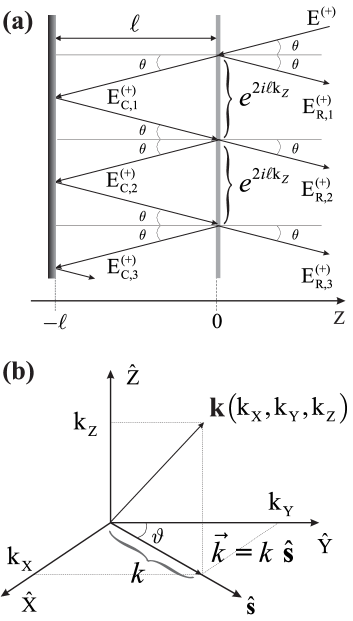
Figure 1: (Color online) (a) Multiple-reflections method DK for an incident plane wave that penetrates the planar resonator from the outside. (b) Cylindrical coordinate system in the reciprocal space. See text for details.

In order to describe a two-level atom coupled to a field confined in a planar resonator, we have to consider first an empty resonator and determine the respective quantized electromagnetic field. In this section, we analyze the one-sided leaky cavity with planar geometry as shown in Fig. 1(a). This cavity consists of a perfectly reflecting (solid) plane mirror located at $z=-\ell$ and a leaky (semitransparent) plane mirror located at $z=0$.

As we mentioned in the introduction, there is an essential difference between a resonator with spherical mirrors, used in typical cavity-QED experiments, and a planar resonator. In the latter confinement configuration, only the normal component of wave vector (along the $\mathsf{k}_{z}$-axis) can take discrete values inside a perfectly reflecting (lossless) planar cavity, while the other two components propagate freely. In a leaky planar resonator, in contrast, the semitransparent mirror at $z=0$ causes the cavity relaxation, i.e., the leakage of cavity photons and, therefore, even the $z$-component of wave vector can never become completely discrete. In contrast to the Koshino’s treatment, the cavity relaxation in our approach is not a predefined function. Instead, it is determined by the transmissivity and reflectivity parameters of planar resonator. This enables us to include both the intra-cavity field and the field that leaks outside (or penetrates into the resonator) in the same framework.

II.1 Semitransparent dielectric-slab mirror

Following the conventional approach (see Sec. 5.C in Ref. SC ), we model the semitransparent mirror by an idealized (infinitesimally) thin layer of dielectric material, the so-called dielectric slab, with the dielectric constant around $z=0$ given by

$$\epsilon(z)=\epsilon\left[1+\eta\,\delta(z)\right]\,,$$ (2)

where $\epsilon$ denotes the permittivity of vacuum and $\eta$ is the positive and real parameter that encodes the transparency (see below). In Ref. DK , Dutra and Knight showed that the transmissivity and reflectivity of such a thin dielectric slab are given by the expressions

$$T_{\bot}(\mathbf{k})=\frac{2\,\mathsf{k}_{z}}{2\,\mathsf{k}_{z}-\dot{\iota}\,\mathbf{k}^{2}\,\eta}\,;\quad T_{\parallel}(\mathbf{k})=\frac{2}{2-\dot{\iota}\,\mathsf{k}_{z}\,\eta}\,,\quad$$ (3a)

$$R_{\bot}(\mathbf{k})=\frac{\dot{\iota}\,\mathbf{k}^{2}\,\eta}{2\,\mathsf{k}_{z}-\dot{\iota}\,\mathbf{k}^{2}\,\eta}\,;\quad R_{\parallel}(\mathbf{k})=\frac{\dot{\iota}\,\mathsf{k}_{z}\,\eta}{\dot{\iota}\,\,\mathsf{k}_{z}\,\eta-2}\,,\quad$$ (3b)

which fulfill the equalities

$$\qquad|R_{\alpha}(\mathbf{k})|^{2}+|T_{\alpha}(\mathbf{k})|^{2}=1\,,$$ (4a)

$$R_{\alpha}(\mathbf{k})^{*}\,T_{\alpha}(\mathbf{k})+T_{\alpha}(\mathbf{k})^{*}\,R_{\alpha}(\mathbf{k})=0\,,$$ (4b)

where $\mathbf{k}$ is the wave vector, $\alpha=\bot$ refers to the component normal to the plane of mirror (along the $z$ axis), and $\alpha=\parallel$ refers to the component lying on the plane of mirror ($x-y$ plane).

Using Eqs. (3), one can readily check that the mirror becomes completely transparent in the limit $\eta\rightarrow 0$, while it becomes a perfect reflector in the limit $\eta\rightarrow\infty$, i.e.,

$$T_{\alpha}(\mathbf{k})=\begin{cases}1,\;\eta\rightarrow 0,\\ 0,\;\eta\rightarrow\infty,\end{cases}R_{\alpha}(\mathbf{k})=\begin{cases}0,\;\eta\rightarrow 0,\\ m_{\alpha},\;\eta\rightarrow\infty,\end{cases}$$ (5)

where $m_{\bot}=-1$ and $m_{\parallel}=1$. The parameter $\eta$, therefore, determines alone the transmissivity and reflectivity of the (leaky) mirror.

In our scheme, the leaky mirror at $z=0$ ensures also that a light pulse can penetrate the resonator from outside. The leaky mirror, therefore, is supposed to have a high but non-perfect reflectivity ($\eta\gg 1$) which, in this paper, is understood as a small deviation from the perfect reflectivity limit. Since $T_{\alpha}(\mathbf{k})$ and $R_{\alpha}(\mathbf{k})$ are constant in the perfect reflectivity limit [see Eqs. (5)], we can treat (to a good approximation) the transmissivity and reflectivity of a leaky mirror as complex valued constants

$$\qquad T_{\alpha}(\mathbf{k})\cong T_{\alpha}\quad\text{and}\quad R_{\alpha}(\mathbf{k})\cong R_{\alpha}\,;$$ (6a)

$$|R_{\alpha}|^{2}+|T_{\alpha}|^{2}=1\,,\quad R_{\alpha}^{*}\,T_{\alpha}+T_{\alpha}^{*}\,R_{\alpha}=0\,.$$ (6b)

On top of this, moreover, the expressions (3) imply

$$\text{Re}\left(T_{\alpha}\right)\ll\text{Im}\left(T_{\alpha}\right)\quad\text{and}\quad\text{Re}\left(R_{\alpha}\right)\gg\text{Im}\left(R_{\alpha}\right)\,.$$ (7)

The assumption (6a) together with relations (6b) and (7) suggest that $T_{\alpha}$ and $R_{\alpha}$ can be chosen in the form

$$R_{\alpha}=m_{\alpha}\sqrt{1-\tau^{2}}\,;\quad T_{\alpha}=\dot{\iota}\,\,\tau\,,\quad\tau\ll 1\,$$ (8)

in order to describe a leaky mirror that deviates only slightly from the perfect one. This presentation implies that the limit of perfect reflectivity is reproduced up to the first order of $\tau$, i.e., $R_{\alpha}$ starts to deviate from $m_{\alpha}$ to the second order of $\tau$. Throughout this paper, therefore, we consider the expressions (8) to describe a leaky mirror, while the expressions (3) are considered to describe an arbitrarily semitransparent mirror or a perfectly reflecting mirror.

II.2 One-sided planar resonator with a semitransparent mirror

An unconfined light propagates in free space, such that the positive-frequency part of its electric field $\mathbf{E}(\mathbf{r},t)$ is expressed as follows CT

$$\mathbf{E}^{{\text{\tiny(+)}}}(\mathbf{r},t) = \sum_{\alpha}\int d\,\mathbf{k}\,\hat{\mathbf{v}}_{\alpha}(\mathbf{k})\,\mathcal{E}^{{\text{\tiny(+)}}}_{\alpha}(\mathbf{k})\,e^{\dot{\iota}\,(\mathbf{k}\cdot\mathbf{r}-\mathsf{k}c\,t)}$$ (9)

$$\equiv \int d\,\mathbf{k}\,\mathbf{E}^{{\text{\tiny(+)}}}(\mathbf{k},\mathbf{r})\,e^{-\dot{\iota}\,\mathsf{k}c\,t}\,,$$

where $\mathsf{k}\equiv|\mathbf{k}|$ denotes the modulus of wave vector, $\hat{\mathbf{v}}_{\alpha}(\mathbf{k})$ denotes the unit vector specifying the direction of a given electric-field component, while $\mathcal{E}^{{\text{\tiny(+)}}}_{\alpha}(\mathbf{k})$ denote the electric-field amplitude. We calculate how the one-sided planar resonator with a semitransparent mirror modifies the plane waves encoded by the expression $\mathbf{E}^{{\text{\tiny(+)}}}(\mathbf{k},\mathbf{r})$. Having this modified expression, we then insert it back into Eq. (9) along with the quantum counterparts of the field amplitudes $\mathcal{E}^{{\text{\tiny(+)}}}_{\alpha}(\mathbf{k})$ and determine the quantized electric field in the presence of the resonator. With the help of quantized electric and magnetic fields, furthermore, we compute the total electromagnetic energy in the physical space that includes regions inside and outside the cavity along with the region occupied by the leaky mirror.

Similar to the theory of a Fabry-Perot resonator BW , we apply the multiple-reflection approach by summing the reflected and transmitted plane waves as depicted in Fig. 1(a). We recall that the solid mirror is a perfectly conducting plane that implies the transformation of the amplitudes of the electric field

$$\mathcal{E}^{{\text{\tiny(+)}}}_{\alpha}(\mathbf{k})\rightarrow m_{\alpha}\,\mathcal{E}^{{\text{\tiny(+)}}}_{\alpha}(\mathbf{k});\quad m_{\bot}=-1,\quad m_{\parallel}=1,$$ (10)

In contrast to the perfect mirror at $z=-\ell$, the action of a semitransparent mirror on the incident plane waves is determined by the reflectivity and transmissivity (3), which imply the respective transformations of the amplitudes of the electric field

$$\mathcal{E}^{{\text{\tiny(+)}}}_{\alpha}(\mathbf{k})\rightarrow R_{\alpha}(\mathbf{k})\,\mathcal{E}^{{\text{\tiny(+)}}}_{\alpha}(\mathbf{k})\,;$$ (11a)

$$\mathcal{E}^{{\text{\tiny(+)}}}_{\alpha}(\mathbf{k})\rightarrow T_{\alpha}(\mathbf{k})\,\mathcal{E}^{{\text{\tiny(+)}}}_{\alpha}(\mathbf{k})\,.$$ (11b)

Using the multiple-reflection approach with relations (10) and (11), we compute the electric field inside ($-\ell\leq z<0$) and outside ($z>0$) the planar cavity region,

$$\mathbf{E}^{{\text{\tiny(+)}}}_{\text{C}}(\mathbf{k},\mathbf{r})=\sum_{i=1}^{\infty}\mathbf{E}^{{\text{\tiny(+)}}}_{\text{C},i}(\mathbf{k},\mathbf{r})$$

$$=2\left[\mathcal{E}^{{\text{\tiny(+)}}}_{\parallel}(\mathbf{k})\,L_{\parallel}(\mathbf{k})\,\cos[\mathsf{k}_{z}(z+\ell)]\,\frac{k}{\mathsf{k}}\,\hat{\mathbf{z}}\right.$$

$$-\dot{\iota}\,\,\mathcal{E}^{{\text{\tiny(+)}}}_{\parallel}(\mathbf{k})\,L_{\parallel}(\mathbf{k})\,\sin[\mathsf{k}_{z}(z+\ell)]\frac{\mathsf{k}_{z}}{\mathsf{k}}\,\hat{\mathbf{s}}$$

$$-\left.\dot{\iota}\,\,\mathcal{E}^{{\text{\tiny(+)}}}_{\bot}(\mathbf{k})\,L_{\bot}(\mathbf{k})\,\sin[\mathsf{k}_{z}(z+\ell)]\,\hat{\mathbf{k}}_{\bot}\right]e^{\dot{\iota}\,\vec{k}\,\cdot\mathbf{r}},$$ (12)

$$\mathbf{E}^{{\text{\tiny(+)}}}_{\text{O}}(\mathbf{k},\mathbf{r})=\mathbf{E}^{{\text{\tiny(+)}}}(\mathbf{k},\mathbf{r})+\sum_{i=1}^{\infty}\mathbf{E}^{{\text{\tiny(+)}}}_{\text{R},i}(\mathbf{k},\mathbf{r})$$

$$=\left[\mathcal{E}^{{\text{\tiny(+)}}}_{\parallel}(\mathbf{k})\left(e^{-\dot{\iota}\,\mathsf{k}_{z}z}+P_{\parallel}(\mathbf{k})\,e^{\dot{\iota}\,\mathsf{k}_{z}z}\right)\,\frac{k}{\mathsf{k}}\,\hat{\mathbf{z}}\right.$$

$$+\mathcal{E}^{{\text{\tiny(+)}}}_{\parallel}(\mathbf{k})\left(e^{-\dot{\iota}\,\mathsf{k}_{z}z}-P_{\parallel}(\mathbf{k})\,e^{\dot{\iota}\,\mathsf{k}_{z}z}\right)\frac{\mathsf{k}_{z}}{\mathsf{k}}\,\hat{\mathbf{s}}$$

$$+\left.\mathcal{E}^{{\text{\tiny(+)}}}_{\bot}(\mathbf{k})\left(e^{-\dot{\iota}\,\mathsf{k}_{z}z}+P_{\bot}(\mathbf{k})\,e^{\dot{\iota}\,\mathsf{k}_{z}z}\right)\hat{\mathbf{k}}_{\bot}\right]e^{\dot{\iota}\,\vec{k}\,\cdot\mathbf{r}},$$ (13)

where $\mathbf{k}=\{\mathsf{k}_{z},k,\vartheta\}$ has been expressed in the cylindrical coordinate basis, while $\vec{k}\,=k\,\hat{\mathbf{s}}$ is the (in-plane) wave vector lying on the plane of mirror as shown in Fig. 1(b). The orthogonal unit vectors $\hat{\mathbf{z}}$, $\hat{\mathbf{s}}$, and $\hat{\mathbf{k}}_{\bot}\equiv\hat{\mathbf{s}}\times\hat{\mathbf{z}}$ determine the polarization of the resulting electric field, while

$$\qquad L_{\alpha}(\mathbf{k})\equiv\frac{T_{\alpha}(\mathbf{k})}{1-e^{2\,\dot{\iota}\,\ell\,\mathsf{k}_{z}}\,m_{\alpha}\,R_{\alpha}(\mathbf{k})}\,,$$ (14a)

$$P_{\alpha}(\mathbf{k})\equiv R_{\alpha}(\mathbf{k})+T_{\alpha}(\mathbf{k})\,L_{\alpha}(\mathbf{k})\,m_{\alpha}\,e^{2\,\dot{\iota}\,\ell\,\mathsf{k}_{z}}$$ (14b)

characterize the spectral response of resonator D .

At this point, we introduce the quantum counterpart of the (positive-frequency) field amplitude

$$\mathcal{E}^{{\text{\tiny(+)}}}_{\alpha}(\mathbf{k})=\sqrt{\frac{2\,\hbar\,\omega_{\mathbf{k}}}{\epsilon(2\pi)^{3}}}\,a_{\alpha}(\mathbf{k})\,,$$ (15)

where $\omega_{\mathbf{k}}\equiv c\,|\mathbf{k}|=c\,\mathsf{k}$, while $a_{\alpha}(\mathbf{k})$ is the photon annihilation operator that satisfies

$$[a_{\alpha}(\mathbf{k}),a^{\dagger}_{\alpha^{\prime}}(\mathbf{k}^{\prime})]=\delta_{\alpha,\alpha^{\prime}}\,\delta\left(\mathbf{k}-\mathbf{k}^{\prime}\right),$$ (16a)

$$\hskip 28.45274pt[a_{\alpha}(\mathbf{k}),a_{\alpha^{\prime}}(\mathbf{k}^{\prime})]=0\,.$$ (16b)

In contrast to the free-space case, the above amplitude contains an extra factor of $2$ due to the perfect mirror restricting the field to the half-space only DK . By inserting Eqs. (12) and (13) along with the amplitude (15) into the integral (9), we obtain the quantized electric field inside $\mathbf{E}^{{\text{\tiny(+)}}}_{\text{C}}(\mathbf{r},t)$ and outside the cavity $\mathbf{E}^{{\text{\tiny(+)}}}_{\text{O}}(\mathbf{r},t)$ region,

$$\mathbf{E}^{{\text{\tiny(+)}}}_{\bullet}(\mathbf{r},t)=$$ (17)

$$=\sum_{\alpha}\int^{\prime}d\,\mathbf{k}\sqrt{\frac{2\,\hbar\,\omega_{\mathbf{k}}}{\epsilon(2\pi)^{3}}}\,\mathbf{U}_{\alpha,\bullet}(\mathbf{k},z)\,a_{\alpha}(\mathbf{k})\,e^{\dot{\iota}\,(\vec{k}\,\cdot\mathbf{r}-\omega_{\mathbf{k}}t)},$$

where the integration (prime symbol) is restricted to the positive $\mathsf{k}_{z}$, while the subscript $\bullet$ denote C or O depending on the region inside or outside the cavity, respectively. In this expression,

$$\mathbf{U}_{\bot,\text{C}}(\mathbf{k},z) = -2\,\dot{\iota}\,\,L_{\bot}(\mathbf{k})\,\sin[\mathsf{k}_{z}(z+\ell)]\,\hat{\mathbf{k}}_{\bot}\,;$$ (18a)

$$\mathbf{U}_{\bot,\text{O}}(\mathbf{k},z) = \left(e^{-\dot{\iota}\,\mathsf{k}_{z}z}+P_{\bot}(\mathbf{k})\,e^{\dot{\iota}\,\mathsf{k}_{z}z}\right)\hat{\mathbf{k}}_{\bot}\,;$$ (18b)

$$\mathbf{U}_{\parallel,\text{C}}(\mathbf{k},z) = 2\,L_{\parallel}(\mathbf{k})\,\left(\cos[\mathsf{k}_{z}(z+\ell)]\,\frac{k}{\mathsf{k}}\,\hat{\mathbf{z}}\right.$$ (18c)

$$- \left.\dot{\iota}\,\,\sin[\mathsf{k}_{z}(z+\ell)]\frac{\mathsf{k}_{z}}{\mathsf{k}}\,\hat{\mathbf{s}}\right)\,;$$

$$\mathbf{U}_{\parallel,\text{O}}(\mathbf{k},z) = \left(e^{-\dot{\iota}\,\mathsf{k}_{z}z}+P_{\parallel}(\mathbf{k})\,e^{\dot{\iota}\,\mathsf{k}_{z}z}\right)\frac{k}{\mathsf{k}}\,\hat{\mathbf{z}}$$ (18d)

$$+ \left(e^{-\dot{\iota}\,\mathsf{k}_{z}z}-P_{\parallel}(\mathbf{k})\,e^{\dot{\iota}\,\mathsf{k}_{z}z}\right)\frac{\mathsf{k}_{z}}{\mathsf{k}}\,\hat{\mathbf{s}}\,.\quad$$

Moreover, the global mode functions

$$\mathbf{U}_{\alpha}(\mathbf{k},\mathbf{r})\equiv e^{\dot{\iota}\,\vec{k}\,\cdot\mathbf{r}}\left[\mathbf{U}_{\alpha,\text{O}}(\mathbf{k},z)+\mathbf{U}_{\alpha,\text{C}}(\mathbf{k},z)\right]$$ (19)

form an orthonormal set

$$\int d\mathbf{r}\,\mathbf{U}_{\alpha}(\mathbf{k},\mathbf{r})\cdot\mathbf{U}^{*}_{\alpha^{\prime}}(\mathbf{k}^{\prime},\mathbf{r})=(2\pi)^{3}\,\delta_{\alpha,\alpha^{\prime}}\,\delta\left(\mathbf{k}-\mathbf{k}^{\prime}\right)\,,$$ (20)

where the integration over the $z$-axis is restricted to $-\ell<z<\infty$. Using the electric field (17), we readily obtain the magnetic field inside and outside the cavity region,

$$\mathbf{B}^{{\text{\tiny(+)}}}_{\bullet}(\mathbf{r},t)=$$ (21)

$$=\sum_{\alpha}\int^{\prime}d\,\mathbf{k}\sqrt{\frac{2\,\hbar\,\omega_{\mathbf{k}}}{c\,\epsilon(2\pi)^{3}}}\mathbf{V}_{\alpha,\bullet}(\mathbf{k},z)\,a_{\alpha}(\mathbf{k})\,e^{\dot{\iota}\,(\vec{k}\,\cdot\mathbf{r}-\omega_{\mathbf{k}}t)},$$

where

$$\mathbf{V}_{\alpha,\bullet}(\mathbf{k},z)=\frac{1}{\mathsf{k}}\left(\vec{k}\,-\dot{\iota}\,\hat{\mathbf{z}}\frac{\partial}{\partial z}\right)\times\mathbf{U}_{\alpha,\bullet}(\mathbf{k},z)\,.$$ (22)

Owing to the quantized electric (17) and magnetic (21) fields, we compute the energy of the electromagnetic field in the space that includes the regions inside and outside the cavity together with the region occupied by the leaky mirror. This energy is given by the free-field Hamiltonian

$$H_{\text{F}} = \int_{-\infty}^{\infty}dx\,dy\left[\int_{-\ell}^{0}dz\,\mathcal{H}_{\text{C}}(\mathbf{r},t)\right.$$ (23)

$$+ \left.\int_{0}^{\infty}dz\,\mathcal{H}_{\text{O}}(\mathbf{r},t)+\lim_{\xi\rightarrow\,0}\int_{-\xi}^{\xi}dz\,\mathcal{H}_{\text{L}}(\mathbf{r},t)\right]\,,\quad$$

where $\mathcal{H}_{\text{C}}(\mathbf{r},t)$ and $\mathcal{H}_{\text{O}}(\mathbf{r},t)$ are the energy densities of the electromagnetic fields inside and outside the cavity region, respectively, while $\mathcal{H}_{\text{L}}(\mathbf{r},t)$ is the energy density associated with the leaky mirror. Since the electric field vanishes inside a perfectly reflecting mirror, there is no extra contribution to (23). By following the approach of Ref. D , it can be shown that the above Hamiltonian takes the expected form

$$H_{\text{F}}=\sum_{\alpha}\int^{\prime}d\,\mathbf{k}\,\frac{\hbar\,\omega_{\mathbf{k}}}{2}\left[a_{\alpha}^{\dagger}(\mathbf{k})\,a_{\alpha}(\mathbf{k})+a_{\alpha}(\mathbf{k})\,a_{\alpha}^{\dagger}(\mathbf{k})\right]$$ (24)

and describes the energy of an infinite set of harmonic oscillators each characterized by the frequency $\omega_{\mathbf{k}}$.

II.3 The limit of perfect reflectivity

In the previous section, we derived the quantized electric and magnetic fields in the presence of a one-sided planar resonator as displayed in Fig. 1(a) with an arbitrarily semitransparent mirror. We found that the energy of the electromagnetic field, localized inside and outside the cavity and inside the semitransparent mirror, is given by the Hamiltonian (24). In this section, we reconsider the obtained results in the (lossless) limit of perfect reflectivity, i.e., when the leaky mirror at $z=0$ becomes a perfectly reflecting mirror ($\eta\rightarrow\infty$). In this case, two types of photon field operators, acting in the intra-cavity region and outside region (reservoir) emerge from the global photon operator $a_{\alpha}(\mathbf{k})$. In the next sections, we consider these operators for the case of a leaky cavity given by the condition $\tau\ll 1$ and understood as a small deviation from the perfect-reflectivity case.

In order to proceed, we express Eq. (17) in the form

$$\mathbf{E}^{{\text{\tiny(+)}}}_{\text{C}}(\mathbf{r},t) = \sum_{\alpha}\int^{\prime}d\,\mathbf{k}\sqrt{\frac{2\,\ell\,\hbar\;\omega_{\mathbf{k}}}{\pi\,\epsilon\,(2\pi)^{3}}}\times$$

$$\qquad\widetilde{\mathbf{U}}_{\alpha,\text{C}}(\mathbf{k},z)\,|L_{\alpha}(\mathbf{k})|^{2}\,\tilde{a}_{\alpha}(\mathbf{k})\,e^{\dot{\iota}\,(\vec{k}\,\cdot\mathbf{r}-\omega_{\mathbf{k}}\,t)}\,,$$

where we introduced $\mathbf{U}_{\alpha,\text{C}}(\mathbf{k},z)\equiv L_{\alpha}(\mathbf{k})\,\widetilde{\mathbf{U}}_{\alpha,\text{C}}(\mathbf{k},z)$ and

$$a_{\alpha}(\mathbf{k})\equiv\sqrt{\ell/\pi}\,L^{*}_{\alpha}(\mathbf{k})\,\tilde{a}_{\alpha}(\mathbf{k})\,.$$ (26)

In the perfect-reflectivity limit, it was showed by Dutra and Knight in Ref. DK that

$$\lim_{\eta\rightarrow\infty}|L_{\alpha}(\mathbf{k})|^{2}=\frac{\pi}{\ell}\sum_{n=-\infty}^{\infty}\delta\left(\mathsf{k}_{z}-\mathsf{k}_{z,n}\right),$$ (27)

where $\mathsf{k}_{z,n}\equiv n\,\pi/\ell$. By inserting this expression into Eq. (II.3) and integrating over $\mathsf{k}_{z}$, we obtain the electric field inside the cavity in the limit of perfect reflectivity,

$$\mathbf{E}^{{\text{\tiny(+)}}}_{\text{CL}}(\mathbf{r},t) = \sum_{\alpha,n}\int d\vec{k}\,\,\sqrt{\frac{\hbar\;\omega_{n,k}}{\epsilon(2\pi)^{2}\,\ell}}\times$$

$$\widetilde{\mathbf{U}}_{\alpha,\text{C}}(\mathsf{k}_{z,n},\vec{k}\,,z)\,\tilde{a}_{\alpha}(\mathsf{k}_{z,n},\vec{k}\,)\,e^{\dot{\iota}\,(\vec{k}\,\cdot\mathbf{r}-\omega_{n,k}t)},$$

where $\omega_{n,k}\equiv c\sqrt{\mathsf{k}_{z,n}^{2}+k^{\,2}}$ is the (quasi-mode) frequency, and where the reduced mode functions $\widetilde{\mathbf{U}}_{\alpha,\text{C}}$ form an orthogonal set

$$\int dz\,\widetilde{\mathbf{U}}_{\alpha,\text{C}}(\mathsf{k}_{z,n},\vec{k}\,,z)\cdot\widetilde{\mathbf{U}}^{*}_{\alpha^{\prime},\text{C}}(\mathsf{k}_{z,n^{\prime}},\vec{k}\,,z)=2\,\ell\;\delta_{n,n^{\prime}}\,\delta_{\alpha,\alpha^{\prime}}\,$$ (29)

with the integration being restricted to $-\ell<z<0$.

The photon annihilation operator $\tilde{a}_{\alpha}(\mathsf{k}_{z,n},\vec{k}\,)$ in Eq. (II.3) depends on the discrete values of $n$ and continuous values of $\vec{k}\,$. Although the expression $\mathbf{E}^{{\text{\tiny(+)}}}_{\text{CL}}(\mathbf{r},t)$ is formally identical to the (positive-frequency parts of) electric field inside a lossless planar resonator (see Ref. DK ), we remind that the operator $\tilde{a}_{\alpha}(\mathsf{k}_{z,n},\vec{k}\,)$ has been obtained from $a_{\alpha}(\mathbf{k})$ using the definition (26) and the discretization of $\mathsf{k}_{z}$ component. In order to define the cavity operator acting inside the cavity region only, we keep Eq. (II.3) with replacing $\tilde{a}_{\alpha}(\mathsf{k}_{z,n},\vec{k}\,)$ by operator $c_{\alpha,n}(\vec{k}\,)$,

$$\mathbf{E}^{{\text{\tiny(+)}}}_{\text{CP}}(\mathbf{r},t) = \sum_{\alpha,n}\int d\vec{k}\,\,\sqrt{\frac{\hbar\;\omega_{n,k}}{\epsilon(2\pi)^{2}\,\ell}}\times$$

$$\qquad\widetilde{\mathbf{U}}_{\alpha,\text{C}}(\mathsf{k}_{z,n},\vec{k}\,,z)\,c_{\alpha,n}(\vec{k}\,)\,e^{\dot{\iota}\,(\vec{k}\,\cdot\mathbf{r}-\omega_{n,k}t)}\,,$$

where we interpret $c_{\alpha,n}(\vec{k}\,)$ as the cavity photon annihilation operator that satisfies

$$[c_{\alpha,n}(\vec{k}\,),c^{\dagger}_{\alpha^{\prime},n^{\prime}}(\vec{k}\,^{\prime})]=\delta_{\alpha,\alpha^{\prime}}\,\delta_{n,n^{\prime}}\,\delta\left(\vec{k}\,-\vec{k}\,^{\prime}\right),$$ (31a)

$$\hskip 42.67912pt[c_{\alpha,n}(\vec{k}\,),c_{\alpha^{\prime},n^{\prime}}(\vec{k}\,^{\prime})]=0\,,$$ (31b)

and is characterized by the quasi-mode frequency $\omega_{n,k}$.

In order to derive $c_{\alpha,n}(\vec{k}\,)$ in terms of global operator $a_{\alpha}(\mathbf{k})$, we multiply (scalarly) both Eqs. (17) and (II.3) by $\widetilde{\mathbf{U}}^{*}_{\alpha,\text{C}}(\mathsf{k}_{z,n^{\prime}},\vec{k}\,,z)$ and integrate them over $z$ from $-\ell$ to $0$ using the property (29). We equate the resulting expressions and solve them for the operator $c_{\alpha,n}(\vec{k}\,)$,

$$c_{\alpha,n}(\vec{k}\,)=\frac{1}{2\,\sqrt{\pi\,\ell}}\int^{\prime}d\,\mathsf{k}_{z}\sqrt{\frac{\omega_{\mathbf{k}}}{\omega_{n,k}}}\,L_{\alpha}(\mathbf{k})\,a_{\alpha}(\mathbf{k})\times$$ (32)

$$\qquad e^{\dot{\iota}\,(\omega_{n,k}-\omega_{\mathbf{k}})\,t}\int dz\;\widetilde{\mathbf{U}}_{\alpha,\text{C}}(\mathsf{k}_{z},\vec{k}\,,z)\cdot\widetilde{\mathbf{U}}^{*}_{\alpha,\text{C}}(\mathsf{k}_{z,n},\vec{k}\,,z)\,,$$

which obeys the commutation relations (31).

In a similar fashion, we derive the electric field valid outside the cavity region only. For this, we first express $\mathbf{E}^{{\text{\tiny(+)}}}_{\text{O}}(\mathbf{r},t)$ [see Eq. (17)] in the limit $\eta\rightarrow\,\infty$ [see Eq. (5)],

$$\mathbf{E}^{{\text{\tiny(+)}}}_{\text{OL}}(\mathbf{r},t) = \sum_{\alpha}\int^{\prime}d\,\mathbf{k}\sqrt{\frac{2\hbar\;\omega_{\mathbf{k}}}{\epsilon(2\pi)^{3}}}\times$$ (33)

$$\qquad\widetilde{\mathbf{U}}_{\alpha,\text{O}}(\mathbf{k},z)\,a_{\alpha}(\mathbf{k})\,e^{\dot{\iota}\,(\vec{k}\,\cdot\mathbf{r}-\omega_{\mathbf{k}}t)}\,,$$

where the reduced mode functions

$$\widetilde{\mathbf{U}}_{\alpha,\text{O}}(\mathbf{k},z)\equiv\lim_{\eta\rightarrow\,\infty}\mathbf{U}_{\alpha,\text{O}}(\mathbf{k},z)=\widetilde{\mathbf{U}}_{\alpha,\text{C}}(\mathbf{k},z-\ell)$$

form an orthonormal set

$$\int dz\,\widetilde{\mathbf{U}}_{\alpha,\text{O}}(\mathsf{k}_{z},\vec{k}\,,z)\cdot\widetilde{\mathbf{U}}^{*}_{\alpha^{\prime},\text{O}}(\mathsf{k}_{z}^{\prime},\vec{k}\,,z)=2\pi\;\delta_{\alpha,\alpha^{\prime}}\,\delta(\mathsf{k}_{z}-\mathsf{k}_{z}^{\prime})\,,$$ (34)

with the integration being restricted to $0<z<\infty$.

By following the same approach as before, we keep Eq. (33) with replacing $a_{\alpha}(\mathbf{k})$ by operator $b_{\alpha}(\mathbf{k})$

$$\mathbf{E}^{{\text{\tiny(+)}}}_{\text{OP}}(\mathbf{r},t) = \sum_{\alpha}\int^{\prime}d\,\mathbf{k}\sqrt{\frac{2\hbar\;\omega_{\mathbf{k}}}{\epsilon(2\pi)^{3}}}\times$$ (35)

$$\qquad\widetilde{\mathbf{U}}_{\alpha,\text{O}}(\mathbf{k},z)\,b_{\alpha}(\mathbf{k})\,e^{\dot{\iota}\,(\vec{k}\,\cdot\mathbf{r}-\omega_{\mathbf{k}}t)},$$

where we interpret $b_{\alpha}(\mathbf{k})$ as the photon annihilation operator of the (reservoir) modes outside the cavity. This operator satisfies the usual commutation relations

$$[b_{\alpha}(\mathbf{k}),b^{\dagger}_{\alpha^{\prime}}(\mathbf{k}^{\prime})]=\delta_{\alpha,\alpha^{\prime}}\,\delta\left(\mathbf{k}-\mathbf{k}^{\prime}\right),$$ (36a)

$$\hskip 28.45274pt[b_{\alpha}(\mathbf{k}),b_{\alpha^{\prime}}(\mathbf{k}^{\prime})]=0\,.$$ (36b)

In order to find the reservoir photon operator $b_{\alpha}(\mathbf{k})$ in terms of $a_{\alpha}(\mathbf{k})$, we multiply (scalarly) both Eqs. (17) and (35) by $\widetilde{\mathbf{U}}^{*}_{\alpha,\text{O}}(\mathsf{k}_{z}^{\prime},\vec{k}\,,z)$ and integrate them over $z$ from $0$ to $\infty$ using the property (34). We equate the resulting expressions and solve them for the operator $b_{\alpha}(\mathbf{k})$,

$$b_{\alpha}(\mathbf{k})=\frac{1}{2\,\pi}\int^{\prime}d\,\mathsf{k}_{z}^{\prime}\sqrt{\frac{\omega^{\prime}_{\mathbf{k}}}{\omega_{\mathbf{k}}}}\,a_{\alpha}(\mathsf{k}_{z}^{\prime},\vec{k}\,)\times$$ (37)

$$\qquad e^{\dot{\iota}\,(\omega_{\mathbf{k}}-\omega^{\prime}_{\mathbf{k}})\,t}\int d\,z\,\mathbf{U}_{\alpha,\text{O}}(\mathsf{k}_{z}^{\prime},\vec{k}\,,z)\cdot\widetilde{\mathbf{U}}^{*}_{\alpha,\text{O}}(\mathsf{k}_{z},\vec{k}\,,z)\,,$$

where $\omega^{\prime}_{\mathbf{k}}\equiv c\sqrt{\mathsf{k}_{z}^{\prime}+k^{\,2}}$ and which obeys the commutation relations (36).

The relations (29) and (34) along with the commutation relations (31) and (36) imply that the electric fields $\mathbf{E}_{\text{CP}}(\mathbf{r},t)$ and $\mathbf{E}_{\text{OP}}(\mathbf{r},t)$, along with the respective magnetic fields, enable to describe any physically achievable configuration of the electromagnetic field inside and outside the planar resonator, respectively. Except for the region filled by the semitransparent mirror, therefore, the operators $c_{\alpha,n}(\vec{k}\,)$ and $b_{\alpha}(\mathbf{k})$ cover the entire continuum of Fock spaces spanned by the global operator $a_{\alpha}(\mathbf{k})$. In other words, this operator can be expanded as

$$a_{\alpha}(\mathbf{k})=\sum_{n}A_{\alpha,n}(\mathbf{k})\,c_{\alpha,n}(\vec{k}\,)+\int^{\prime}d\,\mathsf{k}_{z}^{\prime}B_{\alpha}(\mathbf{k},\mathsf{k}_{z}^{\prime})b_{\alpha}(\mathsf{k}_{z}^{\prime},\vec{k}\,),$$ (38)

where $A_{\alpha,n}(\mathbf{k})$ and $B_{\alpha}(\mathbf{k},\mathsf{k}_{z}^{\prime})$ are defined by the means of commutators

$$A_{\alpha,n}(\mathbf{k})=\left[a_{\alpha}(\mathbf{k}),\int d\vec{k}\,^{\prime}\,c^{\dagger}_{\alpha,n}(\vec{k}\,^{\prime})\right]\,,$$ (39a)

$$B_{\alpha}(\mathbf{k},\mathsf{k}_{z}^{\prime})=\left[a_{\alpha}(\mathbf{k}),\int d\vec{k}\,^{\prime}\,b^{\dagger}_{\alpha}(\mathbf{k}^{\prime})\right]\,.$$ (39b)

Since the global photon operator obeys the eigenoperator equation $\left[a_{\alpha}(\mathbf{k}),H_{\text{F}}\right]=\hbar\,\omega_{\mathbf{k}}\,a_{\alpha}(\mathbf{k})$ [see Eq. (24)], the expansion (38) can be traced back to Fano’s diagonalization technique utilized in Ref. pr124 to analyze a coupled bound-continuum system. In the framework of cavity QED, this technique has been exhaustively studied in Ref. BR , where $a_{\alpha}(\mathbf{k})$, $c_{\alpha,n}(\vec{k}\,)$, and $b_{\alpha}(\mathbf{k})$ were identified as the dressed, bare (or quasi-cavity), and reservoir photon operators, respectively (see also Ref. oc68 ).

II.4 The case of a high but finite reflectivity

We found above that $a_{\alpha}(\mathbf{k})$ can be expressed with the help of operators $c_{\alpha,n}(\vec{k}\,)$, $b_{\alpha}(\mathbf{k})$ and functions (39). This expected result, obtained for a lossless resonator, is based on the ability to describe any attainable electromagnetic field configuration inside or outside the resonator using the expression (II.3) or (35), respectively.

In this section, we show that the expansion (38) holds true also in the case of a high but finite reflectivity, i.e., a leaky cavity. In order to proceed, we replace the functions $R_{\alpha}(\mathbf{k})$ and $T_{\alpha}(\mathbf{k})$ in (II.3) and (35) by the expressions (8). The structure of $\mathbf{E}^{{\text{\tiny(+)}}}_{\text{CP}}(\mathbf{r},t)$ and $\mathbf{E}^{{\text{\tiny(+)}}}_{\text{OP}}(\mathbf{r},t)$ implies that the reduced mode functions $\widetilde{\mathbf{U}}_{\alpha,\text{C}}(\mathsf{k}_{z,n},\vec{k}\,,z)$, $\widetilde{\mathbf{U}}_{\alpha,\text{O}}(\mathbf{k},z)$ and the orthogonality relations (29), (34) remain unchanged. The operators $c_{\alpha,n}(\vec{k}\,)$ and $b_{\alpha}(\mathbf{k})$, in contrast, include implicitly the reflectivity and transmissivity by means of the spectral response function $L_{\alpha}(\mathbf{k})$ [see Eqs. (14)]. In the case of a leaky cavity with $\tau\ll 1$, to a good approximation, this response function takes the form

$$L(\omega,k)\cong\frac{c}{2\,\ell}\sum_{n=0}^{\infty}\frac{-\tau}{\omega-\omega_{n,k}+\dot{\iota}\,c\,\tau^{2}/(4\,\ell)}\,,$$ (40)

where, without loss of generality, we replaced $\mathsf{k}_{z}$ by the (frequency valued) parameter $\omega$ divided by $c$. In the denominator of this expression, moreover, we have imposed the $k$ dependence by means of the quasi-mode frequency $\omega_{n,k}$. In the limit of vanishing $k$, the resulting function reduces to Eq. (9.49) derived in Ref. D for the case of an one-dimensional leaky cavity, where the contribution of continuous and unconfined modes has been omitted.

By inserting (40) in Eqs. (32) and (37) with replacement $\mathsf{k}_{z}\rightarrow\omega/c$, we compute explicitly $c_{\alpha,n}(\vec{k}\,)$ and $b_{\alpha}(\mathbf{k})$,

$$c_{\alpha,n}(\vec{k}\,)=\int^{\prime}d\omega\,\frac{-\tau/(2\,\sqrt{\pi\,\ell})}{\omega-\omega_{n,k}+\dot{\iota}\,c\,\tau^{2}/(4\,\ell)}\,a_{\alpha}(\omega,\vec{k}\,)\,,$$ (41)

$$b_{\alpha}(\mathbf{k})=\int^{\prime}d\omega\,\,a_{\alpha}(\omega,\vec{k}\,)\left[\delta\left(c\,\mathsf{k}_{z}-\omega\right)\right.$$

$$\quad\quad+\left.\lim_{\xi\rightarrow 0^{+}}\frac{1}{c\,\mathsf{k}_{z}-\omega-\dot{\iota}\,\xi}\,\sum_{n=0}^{\infty}\frac{-\tau^{2}/(4\,\pi\,\ell)}{\omega-\omega_{n,k}+\dot{\iota}\,c\,\tau^{2}/(4\,\ell)}\right],$$

where the global photon operator fulfills the relations

$$[a_{\alpha}(\omega,\vec{k}\,),a^{\dagger}_{\alpha^{\prime}}(\omega^{\prime},\vec{k}\,^{\prime})]=c\,\,\delta_{\alpha,\alpha^{\prime}}\,\delta\left(\omega-\omega^{\prime}\right)\,\delta\left(\vec{k}\,-\vec{k}\,^{\prime}\right),$$

$$\hskip 56.9055pt[a_{\alpha}(\omega,\vec{k}\,),a_{\alpha^{\prime}}(\omega^{\prime},\vec{k}\,^{\prime})]=0\,.$$

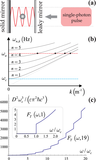
Figure 2: (Color online) (a) Schematic view of the experimental setup that realizes the proposed scenario. (b) Series of branches which characterize the dispersion relation $\omega_{n,k}=c\sqrt{\mathsf{k}_{z,n}^{2}+k^{2}}$ associated with the frequency of cavity quasi-modes. (c) The total form-factor (63) for $N=1$ and $N=19$ being summed over the polarizations. See text for details.

We show below that these operators fulfill the commutation relations (31) and (36), respectively. Using the same arguments as in the previous section, i.e., the possibility to describe any configuration of the electromagnetic field using (II.3) and (35), we conclude that the expansion

$$a_{\alpha}(\omega,\vec{k}\,)=\sum_{n}A_{n}(\omega,k)\,c_{\alpha,n}(\vec{k}\,)+\int^{\prime}d\,\mathsf{k}_{z}\,B(\omega,\mathsf{k}_{z})\,b_{\alpha}(\mathbf{k})$$ (43)

replaces Eq. (38) in the case of a leaky cavity, where

$$A_{n}(\omega,k)=\frac{-\tau/(2\,\sqrt{\pi\,\ell})}{\omega-\omega_{n,k}-\dot{\iota}\,c\,\tau^{2}/(4\,\ell)}\,,$$ (44a)

$$B(\omega,\mathsf{k}_{z})=\delta\left(c\,\mathsf{k}_{z}-\omega\right)$$

$$\hskip 28.45274pt+\lim_{\xi\rightarrow 0^{+}}\frac{\tau/(2\,\sqrt{\pi\,\ell})}{c\,\mathsf{k}_{z}-\omega+\dot{\iota}\,\xi}\,\sum_{n=0}^{\infty}A_{n}(\omega,k)\,.\qquad$$ (44b)

In order to show that $c_{\alpha,n}(\vec{k}\,)$ and $b_{\alpha}(\mathbf{k})$ satisfy the commutation relations, we first use Eqs. (41) and (44a), for which the commutator (31a) reduces to the expression

$$\delta_{\alpha,\alpha^{\prime}}\,\delta_{n,n^{\prime}}\,\delta\left(\vec{k}\,-\vec{k}\,^{\prime}\right)\int^{\prime}d\omega\,c\,|A_{n}(\omega,k)|^{2}.$$ (45)

Now we use Eqs. (II.4) and (44b), for which the commutator (36a) reduces to the expression

$$\delta_{\alpha,\alpha^{\prime}}\,\delta\left(\vec{k}\,-\vec{k}\,^{\prime}\right)\int^{\prime}d\omega\,c\,B(\omega,\mathsf{k}_{z}^{\prime})\,B^{*}(\omega,\mathsf{k}_{z})\,.$$ (46)

It can be readily checked that the integral in (45) is equal to one, while the integral in (46) is equal to $\delta\left(\mathsf{k}_{z}-\mathsf{k}_{z}^{\prime}\right)$ up to the contribution $\mathcal{O}(\tau^{4})$, which is negligibly small due to the (leaky cavity) condition $\tau\ll 1$.

III Form-factors and the cavity-QED parameters

In the introduction, we explained that an interacting system of three constituents: (i) an atom coupled to (ii) a planar resonator, and (iii) an input pulse that penetrates the resonator from outside, can exhibit Rabi oscillations reproducing the cavity-QED evolution. In Fig. 2(a) we display the experimental setup that could realize this scenario. In this setup, an atom at rest is located inside the planar resonator, while the single-photon wave packet

$$|\text{in}\rangle=\sum_{\alpha}\int d\mathbf{r}\,\psi(z)\,\varphi_{\alpha}(x,y)\,\tilde{b}^{\dagger}_{\alpha}(\mathbf{r})\,|\text{vac}\rangle$$ (47)

characterized by a non-trivial spatial distribution penetrates the resonator at normal incidence. Here $\tilde{b}_{\alpha}(\mathbf{r})$ denotes the Fourier transform of $b_{\alpha}(\mathbf{k})$, while $|\text{vac}\rangle$ is the photon field vacuum state, such that $a_{\alpha}(\mathbf{k})|\text{vac}\rangle=0$. The functions $\psi(z)$ and $\varphi_{\alpha}(x,y)$ describing the spatial distribution of the light pulse are normalized, such that

$$\int dz\,|\psi(z)|^{2}=\sum_{\alpha}\int dx\,dy\,|\varphi_{\alpha}(x,y)|^{2}=1\,,$$ (48)

and where $|\psi(z)|^{2}$ is localized in the $z>0$ region.

Similar to the standard cavity-QED, the coupled atom-cavity-pulse system is described by a set of parameters which characterize completely the coherent (unitary) and incoherent (non-unitary) parts of its evolution. Before we identify this set, we formulate two criteria by which we determine these parameters. First, this set should contain only three elements with the same physical meaning as the cavity-QED parameters $(g,\,\kappa,\,\gamma)$. This requirement would establish a one-to-one correspondence to the conventional cavity-QED framework. Secondly, these parameters have to depend not only on the atom and cavity characteristics (as in cavity-QED) but also on the lateral profile $\varphi_{\alpha}(x,y)$ of the single-photon pulse (47).

The identification of these parameters, framed by the above two criteria, was proposed by Koshino in Ref. K . In this reference, the author observed that the atom-field coupling extracted from the total Hamiltonian including an atom, the light field, and the atom-cavity interaction encodes the entire triplet of parameters. Using the so-called form-factor formalism that gives a proper framework to isolate and study various couplings of a given Hamiltonian, Koshino calculated the cavity-QED parameters in question and demonstrated that the atomic decay rate $\gamma$ becomes considerably suppressed once the lateral profile $\varphi_{\alpha}(x,y)$ of the input single-photon pulse is appropriately tailored.

However, Koshino introduced four simplifying assumptions in his framework, namely, (i) the evolution of the coupled atom-cavity-pulse system was described by an ad hoc Hamiltonian, (ii) the light field had only one (fixed) polarization, (iii) the atom was described by an averaged (in space) dipole, while (iv) the planar resonator accommodated only one atomic wavelength. In the generalized framework we derived in the previous section, the first two simplifications have been already excluded. In this section, we avoid the remaining two assumptions and generalize, in this way, the paper of Koshino.

III.1 Input light-pulse coupled to the resonator

The light pulse (47) can be expressed in $\mathbf{k}$-space as

$$|\text{in}\rangle=\sum_{\alpha}\int d\,\mathbf{k}\,\widetilde{\psi}(\mathsf{k}_{z})\,\widetilde{\varphi}_{\alpha}(\vec{k}\,)\,b^{\dagger}_{\alpha}(\mathbf{k})|\text{vac}\rangle\,,$$ (49)

where $\widetilde{\psi}(\mathsf{k}_{z})$ and $\widetilde{\varphi}_{\alpha}(\vec{k}\,)$ are the Fourier transforms of $\psi(z)$ and $\varphi_{\alpha}(x,y)$, respectively, and describe the frequency distribution of the input light pulse in $\mathbf{k}$-space. Similar to Eq. (48), these two functions are normalized

$$\int d\,\mathsf{k}_{z}\,|\widetilde{\psi}(\mathsf{k}_{z})|^{2}=\sum_{\alpha}\int d\vec{k}\,\,|\widetilde{\varphi}_{\alpha}(\vec{k}\,)|^{2}=1\,.$$ (50)

In the conventional approach BR ; pra42 , a single-photon state with a non-trivial frequency distribution is typically given by the expression $|1\rangle=\int d\omega_{\mathbf{k}}\,\mathcal{G}(\omega_{\mathbf{k}})\,b^{\dagger}(\omega_{\mathbf{k}})|\text{vac}\rangle$, where $\omega_{\mathbf{k}}$ is proportional to the modulus of $\mathbf{k}$. In our case, however, the frequency distribution is given by $\widetilde{\psi}(\mathsf{k}_{z})$ and $\widetilde{\varphi}_{\alpha}(\vec{k}\,)$ depending on different wave-vector components, while the integration is performed over the $\mathbf{k}$-space.

Using (II.4) and (44), we express (49) in the form

$$|\text{in}\rangle=\frac{1}{c}\int d\omega\,\widetilde{\psi}(\omega)\,d^{\dagger}(\omega,\widetilde{\varphi})|\text{vac}\rangle\,,$$ (51)

that is similar to the conventional single-photon state $|1\rangle$ shown above, and where we introduced the pulse operator

$$d(\omega,\widetilde{\varphi}) \equiv \sum_{\alpha}\int d\vec{k}\,\,\widetilde{\varphi}^{\,*}_{\alpha}(\vec{k}\,)\times$$ (52)

$$\left[1+\dot{\iota}\,\tau\sqrt{\frac{\pi}{\ell}}\sum_{n=0}^{\infty}A^{*}_{n}(\omega,k)\right]a_{\alpha}(\omega,\vec{k}\,)\,,\qquad$$

that depends on the lateral profile $\widetilde{\varphi}_{\alpha}$. This operator, moreover, fulfills the commutation relations

$$[d(\omega,\widetilde{\varphi}),d^{\dagger}(\omega^{\prime},\widetilde{\varphi})]=c\,\,\delta\left(\omega-\omega^{\prime}\right);$$ (53a)

$$\hskip 28.45274pt[d(\omega,\widetilde{\varphi}),d(\omega^{\prime},\widetilde{\varphi})]=0\,,$$ (53b)

and exhibits the properties

$$d^{\dagger}(\omega,\widetilde{\varphi})|\text{vac}\rangle = \widetilde{\psi}^{*}(\omega)\,|\text{in}\rangle\,,$$ (54a)

$$d(\omega,\widetilde{\varphi})|\text{in}\rangle = \widetilde{\psi}(\omega)\,|\text{vac}\rangle\,.$$ (54b)

These properties suggest that $d^{\dagger}(\omega,\widetilde{\varphi})$ creates a single-photon state (49) weighted by $\widetilde{\psi}^{*}(\mathsf{k}_{z})$, while $d(\omega,\widetilde{\varphi})$ annihilates the respective state resulting into the vacuum state weighted by $\widetilde{\psi}(\mathsf{k}_{z})$. In order to complete the derivations in this subsection, we invert the relation (52)

$$a_{\alpha}(\omega,\vec{k}\,)=\widetilde{\varphi}_{\alpha}(\vec{k}\,)\left[1-\dot{\iota}\,\tau\sqrt{\frac{\pi}{\ell}}\sum_{n=0}^{\infty}A_{n}(\omega,k)\right]d(\omega,\widetilde{\varphi})\,,$$ (55)

where we used Eq. (50) along with the relation

$$\dot{\iota}\,\tau\sqrt{\frac{\pi}{\ell}}\,\left|A_{n}(\omega,k)\right|^{2}=A^{*}_{n}(\omega,k)-A_{n}(\omega,k)\,.$$ (56)

III.2 Atom coupled to the resonator

In this section, we derive the Hamiltonian that governs the evolution of the intra-cavity field coupled to a two-level atom by using the electric field (II.3) and the photon field operator (41) of a leaky cavity. We consider an atom at rest inside the resonator as displayed in Fig. 2(a). The internal structure of the atom is completely characterized by the states $|g\rangle$ (ground) and $|e\rangle$ (excited), which fulfill the usual orthogonality and completeness relations. We recall that the cavity quasi-modes are characterized by the frequency $\omega_{n,k}$ that has both discrete and continuous contributions. These quasi-modes are grouped by branches indexed by $n$ as can be seen in Fig. 2(b), where $\omega_{c}\equiv\omega_{1,0}=c\,\mathsf{k}_{z,1}$ defines the lower cut-off frequency. We assume that the atomic transition frequency $\omega_{a}$ is equal or above this lower cut-off frequency, such that the atom couples at least to one quasi-mode of the resonator.

We choose the position of atomic center-of-mass $\mathbf{r}^{\prime}=\{0,0,-\ell/2\}$ and switch to the Schrödinger picture, in which the electric field (II.3) is time-independent. In the dipole approximation, the Hamiltonian ($n=1,\ldots,N$)

$$H_{\text{AC}} = -\mathcal{Q}\,\mathbf{r}\cdot\left[\mathbf{E}^{{\text{\tiny(+)}}}_{\text{CP}}(\mathbf{r}^{\prime})+\mathbf{E}^{{\text{\tiny(--)}}}_{\text{CP}}(\mathbf{r}^{\prime})\right]$$ (57)

$$= -\mathcal{D}\left(\sigma^{\dagger}+\sigma\right)\sum_{\alpha,n}^{N}\int d\vec{k}\,\,\sqrt{\frac{\hbar\;\omega_{n,k}}{\epsilon(2\pi)^{2}\,\ell}}\times$$

$$\left[\hat{\boldsymbol{\rho}}\cdot\widetilde{\mathbf{U}}_{\alpha,\text{C}}\left(\mathsf{k}_{z,n},\vec{k}\,,-\frac{\ell}{2}\right)c_{\alpha,n}(\vec{k}\,)+H.c.\right]\quad$$

describes the electric-dipole coupling between a two-level atom and $N$ cavity quasi-modes, where $N$ is the number of intersection points between $\omega_{a}$ and the branches of $\omega_{n,k}$ [see Fig. 2(b)]. In the above Hamiltonian, $\mathcal{Q}$ is the electric charge, $\sigma=|g\rangle\langle e|$ is the atomic (excitation) lowering operator. We also introduced the notation $\langle g|\mathcal{Q}\,\mathbf{r}|e\rangle\equiv\mathcal{D}\,\hat{\boldsymbol{\rho}}$ with $\mathcal{D}$ being the (real) dipole matrix element of the atomic transition and $\hat{\boldsymbol{\rho}}$ being the unit real vector that determines the polarization of transition.

In the rotating-wave approximation, we express the Hamiltonian (57) in the form

$$H_{\text{AC}}=\hbar\,\sum_{\alpha,n}^{N}\int d\vec{k}\,\left[\lambda_{\alpha,n}(\vec{k}\,)\,\sigma^{\dagger}\,c_{\alpha,n}(\vec{k}\,)+H.c.\right]\,,$$ (58)

where we introduced the atom-field coupling

$$\lambda_{\alpha,n}(\vec{k}\,)\equiv-\mathcal{D}\sqrt{\frac{\omega_{n,k}}{\epsilon(2\pi)^{2}\,\ell\,\hbar}}\;\hat{\boldsymbol{\rho}}\cdot\widetilde{\mathbf{U}}_{\alpha,\text{C}}\left(\mathsf{k}_{z,n},\vec{k}\,,-\frac{\ell}{2}\right)\,.$$ (59)

Using (24) and (58), we compose the total Hamiltonian

$$H_{\text{T}} = H_{\text{F}}+H_{\text{A}}$$ (60)

$$+ \hbar\,\sum_{\alpha,n}^{N}\int d\vec{k}\,\left[\lambda_{\alpha,n}(\vec{k}\,)\,\sigma^{\dagger}\,c_{\alpha,n}(\vec{k}\,)+H.c.\right]$$

that governs the evolution of a coupled atom-field system, and where $H_{\text{A}}=\hbar\,\omega_{a}\,\sigma_{z}/2$ denotes the atomic Hamiltonian. Using (41) and (44a), furthermore, the above Hamiltonian takes the (first) equivalent form

$$H_{\text{T}}=H_{\text{F}}+H_{\text{A}} + \hbar\,\sum_{\alpha,n}^{N}\int^{\prime}d\omega\,d\vec{k}\,\left[\lambda_{\alpha,n}(\vec{k}\,)\right.\times$$ (61)

$$\left.A^{*}_{n}(\omega,k)\,\sigma^{\dagger}\,a_{\alpha}(\omega,\vec{k}\,)+H.c.\right].\qquad$$

Using Eqs. (55) and (56), finally, we express the above Hamiltonian in the (second) equivalent form

$$H_{\text{T}}=H_{\text{F}}+H_{\text{A}} + \hbar\,\sum_{\alpha,n}^{N}\int^{\prime}d\omega\,d\vec{k}\,\left[\lambda_{\alpha,n}(\vec{k}\,)\,\widetilde{\varphi}_{\alpha}(\vec{k}\,)\right.\times$$ (62)

$$\left.A_{n}(\omega,k)\,\sigma^{\dagger}\,d(\omega,\widetilde{\varphi})+H.c.\right].\qquad$$

III.3 Form-factors and the cavity-QED parameters

Following the approach of Koshino, we define the total form-factor

$$F_{T}(\omega,N) \equiv \frac{1}{c^{3}\,\hbar^{2}}\sum_{\alpha}\int d\vec{k}\,\left|\langle\text{vac},e|H_{\text{T}}\,a^{\dagger}_{\alpha}(\omega,\vec{k}\,)|\text{vac},g\rangle\right|^{2}$$ (63)

$$= \frac{1}{c}\sum_{\alpha}\int d\vec{k}\,\left|\sum_{n}^{N}\lambda_{\alpha,n}(\vec{k}\,)\,A^{*}_{n}(\omega,k)\right|^{2}\qquad$$

that isolates the coupling between the atom and global photon field $a_{\alpha}(\omega,\vec{k}\,)$.

Assuming that the atomic dipole $\hat{\boldsymbol{\rho}}$ lies in the plane parallel to the mirrors, i.e., $\hat{\boldsymbol{\rho}}\cdot\hat{\mathbf{z}}=0$, we calculate analytically the total form-factor (63)

$$F_{T}(\omega,N) = \frac{\mathcal{D}^{2}\,\omega_{c}^{3}}{\epsilon\,\pi^{2}\hbar\,c^{3}}\sum_{n,\text{odd}}^{N}\left(n^{2}+\frac{\omega^{2}}{\omega_{c}^{2}}\right)\times$$ (64a)

$$\left(\frac{1}{2}+\frac{1}{\pi}\,\arctan\left[\frac{4\,\pi}{\tau^{2}}\left(\frac{\omega}{\omega_{c}}-n\right)\right]\right)\qquad$$

$$\equiv \frac{\mathcal{D}^{2}\,\omega_{c}^{3}}{\epsilon\,\pi^{2}\hbar\,c^{3}}\,F^{\circ}_{T}\left(\frac{\omega}{\omega_{c}},N\right)\,,$$ (64b)

that has the units of frequency, while the summation over $n$ is only over the odd and positive integer values. We display in Fig. 2(c) the total form-factor $F_{T}(\omega,N)$, for $N=1$, $N=19$ and $\tau=10^{-3}$. It is clearly seen that the total form-factor depends on the square of $\omega$ and has a steplike behavior at the points $\omega=n\,\omega_{c}$ ($n=1,3,5,\ldots$). This figure displays the spectral mode density of a lossless (1D confined) planar resonator kav ; D ; MF and, therefore, it reveals the physical meaning of the total form-factor.

The chosen value of $\tau=10^{-3}$ is compatible with the assumptions of Sec. II.A, by which a leaky mirror deviates only slightly from a perfect one. Throughout this paper, therefore, we consider this specific value to evaluate various expressions involving $\tau$. We remark, moreover, that the total form-factor derived by Koshino (see Eq. (15) in Ref. K ) is proportional to $F_{T}(\omega,1)$, however, with an excluded contribution of $\omega^{2}/\omega_{c}^{2}$ since the $\parallel$-component of light polarization was disregarded.

Although we assumed that an input light-pulse penetrates the cavity as shown in Fig. 2(a), the total form-factor (64a) is independent of the lateral profile $\varphi_{\alpha}(x,y)$. We observe, however, that the total Hamiltonian expressed in the form (62) contains two operator pairs $\sigma\,d^{\dagger}(\omega,\widetilde{\varphi})$ and $\sigma^{\dagger}d(\omega,\widetilde{\varphi})$, such that

$$\sigma\,d^{\dagger}(\omega,\widetilde{\varphi})|\text{vac},e\rangle=\widetilde{\psi}^{*}(\omega)\,|\text{in},g\rangle\,,$$ (65a)

$$\sigma^{\dagger}d(\omega,\widetilde{\varphi})|\text{in},g\rangle=\widetilde{\psi}(\omega)\,|\text{vac},e\rangle\,,$$ (65b)

These properties along with the atom-field coupling $\lambda_{\alpha,n}(\vec{k}\,)\,\widetilde{\varphi}_{\alpha}(\vec{k}\,)\,A_{n}(\omega,k)$ suggest that, for an appropriately tailored $\widetilde{\varphi}_{\alpha}(\vec{k}\,)$ [equivalently $\varphi_{\alpha}(x,y)$], the atom-field evolution governed by the Hamiltonian (62) can resemble the evolution of a cavity-QED system, that is

$$e^{-\frac{\dot{\iota}\,}{\hbar}H_{\text{T}}\,t}|\text{in},g\rangle=|\text{vac},e\rangle\,,$$ (66)

where the photon field (52) plays the role of cavity photon field in cavity-QED [see (1)]. In other words, if the single-photon pulse (47) penetrates a planar resonator with an atom in the ground state, then (after a certain time interval $t$) this pulse can be completely absorbed by the atom.

Furthermore, we define the second form-factor

$$F_{C}(\omega,\widetilde{\varphi},N)\equiv\frac{1}{c^{3}\,\hbar^{2}}\left|\langle\text{vac},e|H_{\text{T}}\,d^{\dagger}(\omega,\widetilde{\varphi})|\text{vac},g\rangle\right|^{2}\,,$$ (67)

to which we refer below as the cavity form-factor, since it contains the coupling between an atom and the ($\widetilde{\varphi}_{\alpha}$-dependent) photon field (52) that might reproduce the cavity-QED evolution (66). By inserting the total Hamiltonian (62) into the expression (67), we readily obtain

$$F_{C}(\omega,\widetilde{\varphi},N)=\frac{1}{c}\left|\sum_{n,\alpha}^{N}\int d\vec{k}\,\,\lambda_{\alpha,n}(\vec{k}\,)\,\widetilde{\varphi}_{\alpha}(\vec{k}\,)\,A_{n}\left(\omega,k\right)\right|^{2}.$$ (68)

The cavity-QED like behavior (66), exhibited by the atom-cavity-pulse system with an appropriate input pulse, suggests that the cavity form-factor (68) plays the role of the spectral mode density corresponding to the completely (3D) confined light. In a cavity-QED system with reasonable small losses, in turn, this density produces a resonance peak centered around $\omega_{\circ}$ and described by the Lorentzian

$$\mathcal{L}(\omega)=\frac{\kappa}{2\pi}\frac{g^{2}}{(\omega-\omega_{\circ})^{2}+\kappa^{2}/4}\,,$$ (69)

where its area and the half-width are identified with $g^{2}$ and $\kappa$, respectively kav ; D ; MF . Using this analogy and provided that the cavity form-factor resembles a sharply peaked resonance, we identify the atom-field coupling strength with the expression

$$g(\widetilde{\varphi},N)\equiv\left(\int d\omega\,F_{C}(\omega,\widetilde{\varphi},N)\right)^{\frac{1}{2}}\,,$$ (70)

while the cavity relaxation ratio $\kappa(\widetilde{\varphi},N)$ is identified with the half-width of $F_{C}(\omega,\widetilde{\varphi},N)$.

We notice that in contrast to the total form-factor (63), the modulus in (68) is moved outside the integral. With the help of Cauchy -Schwarz inequality, this feature leads to the relation

$$F_{C}(\omega,\widetilde{\varphi},N)\leq F_{T}(\omega,N)\,.$$ (71)

Since the resonance peak (69) describing the spectral mode density of a cavity-QED system is below the (quadratically growing) curve given by Eq. (64a) and corresponding to the spectral mode density of a planar resonator, both above form-factors are in perfect agreement with the relation (71) and the present discussion.

The above relation suggests the third form-factor,

$$F_{N}(\omega,\widetilde{\varphi},N)\equiv F_{T}(\omega,N)-F_{C}(\omega,\widetilde{\varphi},N)\,,$$ (72)

to which we refer below as the non-cavity form-factor, since it gives the difference between the spectral mode densities of (i) the (1D confined) atom-cavity system and (ii) the atom-cavity-pulse system that behaves as a (3D confined) cavity-QED system with losses. Since the cavity form-factor (68) satisfies the relation (71) and encodes $g(\widetilde{\varphi},N)$ and $\kappa(\widetilde{\varphi},N)$, we identify the expression (72) with the atomic decay rate,

$$\gamma(\omega,\widetilde{\varphi},N)\equiv F_{N}(\omega,\widetilde{\varphi},N)\,.$$ (73)

In accordance with the two criteria we formulated in the beginning of this section, we defined three form-factors characterizing the coherent and incoherent parts of evolution of the coupled atom-cavity-pulse system. Being defined in a similar fashion as in the conventional cavity-QED, these form-factors enable us to compare the overall performance of our setup to an arbitrary cavity-QED system. We recall that the input state (51) is a single-photon state with a non-trivial frequency distribution $\widetilde{\psi}(\omega)$, where the parameter $\omega$ contributes to all the form-factors, while the lateral profile $\widetilde{\varphi}_{\alpha}(\vec{k}\,)$ contributes only to the cavity and non-cavity form-factors. In order to enhance the atom-field interaction, in the next section, we determine the optimal frequency distribution $\widetilde{\psi}^{\text{opt}}$ and the optimal lateral profile $\widetilde{\varphi}^{\text{opt}}_{\alpha}$, for which the atomic decay rate vanishes.

IV Analysis of lateral profiles

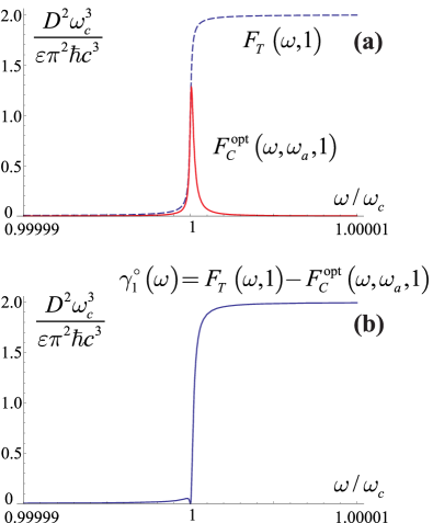
Figure 3: (Color online) (a) The cavity (solid curve) and the total (dashed curve) form-factors for $N=1$ and $f=\omega_{a}$. The cavity form-factor resembles a nice Lorentzian bounded by the total form-factor. (b) The non-cavity form-factor for $N=1$ and $f=\omega_{a}$. See text for details.

In the previous sections, we identified the cavity-QED parameters which characterize both coherent and incoherent parts of the evolution of a coupled atom-cavity-pulse system with losses. We also suggested that the setup displayed in Fig. (2)(a) can reproduce the cavity-QED evolution once an appropriately tailored single-photon pulse and a proper frequency distribution are provided at the input. In this section, we demonstrate that a coupled atom-cavity-pulse system behaves as a cavity-QED system and we evaluate the cavity-QED parameters by considering several predefined pulses.

IV.1 Optimal spatial distribution

Before we evaluate cavity-QED parameters for a predefined single-photon pulse, we determine first $\widetilde{\varphi}^{\text{opt}}_{\alpha}$ and $\widetilde{\psi}^{\text{opt}}$, for which the atomic decay rate vanishes. According to the definition (73), we require the vanishing of the left part of (72). This leads to the equation

$$F_{T}(\omega,N)=F_{C}(\omega,\widetilde{\varphi}^{\text{opt}}_{\alpha},N)\,,$$ (74)

which is an extreme case of Eq. (71). Using Eq. (50) and the cavity form-factor (68), we solve the above equation for the lateral profile. The obtained solution

$$\widetilde{\varphi}^{\text{opt}}_{\alpha}(\vec{k}\,,f,N)=\sum_{n}^{N}\frac{\lambda^{*}_{\alpha,n}(\vec{k}\,)\,A^{*}_{n}\left(f,k\right)}{\sqrt{c\,F_{T}(f,N)}}\,,$$ (75)

fulfills Eq. (50) and depends on the parameters $f$ and $N$.

We insert the above optimal profile back into Eq. (68) and obtain the optimal cavity form-factor

$$F^{\text{opt}}_{C}(\omega,f,N) = \frac{1}{c}\left|\sum_{n,\alpha}^{N}\int d\vec{k}\,\,\lambda_{\alpha,n}(\vec{k}\,)\times\right.$$ (76)

$$\qquad\left.\widetilde{\varphi}^{\text{opt}}_{\alpha}(\vec{k}\,,f,N)\,A_{n}\left(\omega,k\right)\right|^{2}.\qquad$$

Considering, as before, that the atomic dipole $\hat{\boldsymbol{\rho}}$ lies in the plane parallel to the mirrors, we calculate analytically the optimal cavity form-factor (76), which takes the form

$$F^{\text{opt}}_{C}(\omega,f,N)=\frac{\mathcal{D}^{2}\,\omega_{c}^{3}}{\epsilon\,\pi^{2}\hbar\,c^{3}}\left(\frac{\tau}{2\,\pi}\right)^{4}\frac{\left|F^{\circ}_{C}(\frac{\omega}{\omega_{c}},\frac{f}{\omega_{c}},N)\right|^{2}}{F^{\circ}_{T}\left(\frac{f}{\omega_{c}},N\right)}\,,$$ (77)

where $F^{\circ}_{T}(u,N)$ has been defined in (64b), while

$$F^{\circ}_{C}(u,v,N)=$$

$$\sum_{n,\text{odd}}^{N}\left(n^{2}\,\frac{\dot{\iota}\,2\,\pi^{2}+4\,\pi\,\text{arctanh}\left[\frac{4\pi\left(n-\frac{u+v}{2}\right)}{2\pi(v-u)+\dot{\iota}\,\tau^{2}}\right]}{2\,\pi(v-u)+\dot{\iota}\,\tau^{2}}\right.+$$

$$\quad\left.\frac{\dot{\iota}\,2\,\pi^{2}v^{2}+\pi(u+v)\,\text{arctanh}\left[\frac{4\pi\left(n-\frac{u+v}{2}\right)}{2\pi(v-u)+\dot{\iota}\,\tau^{2}}\right]}{2\,\pi(v-u)+\dot{\iota}\,\tau^{2}}\right).\qquad$$ (78)

In Fig. 3(a), we display $F^{\text{opt}}_{C}(\omega,\omega_{a},1)$ by a solid curve that corresponds to the situation, in which the resonator accommodates just one wavelength associated with the atomic transition frequency, that is $\ell=c\,\pi/\omega_{a}$. This implies that only one quasi-mode couples to the atom, that is $\omega_{a}=\omega_{c}$ and $N=1$. It is clearly seen that the solid curve resembles a nice Lorentzian, while the peak of this Lorentzian is bounded by the total form-factor $F_{T}(\omega,1)$ (dashed curve) in agreement with the relation (71). This figure confirms the identification of the cavity form-factor (68) with the spectral mode density of a cavity-QED system with losses. Moreover, this figure reveals the role of parameter $f$ in Eq. (77), and namely, this parameter sets the central frequency of the resulting Lorentzian (solid curve). In Fig. 3(b), furthermore, we display the non-cavity form-factor $F_{T}(\omega,1)-F^{\text{opt}}_{C}(\omega,\omega_{a},1)$ that is identified with the (optimal) atomic decay rate $\gamma^{\circ}_{1}(\omega)$. It can be clearly seen that the atomic decay is efficiently suppressed in the region $\omega\leq\omega_{c}$. This restriction, in turn, suggests the profile of the frequency distribution $\widetilde{\psi}^{\text{opt}}(\omega)$.

We conclude that our system in Fig. 2(a) behaves as a cavity-QED system once the optimal single-photon pulse

$$|\text{opt}_{1}\rangle=\sum_{\alpha}\int d\,\mathbf{k}\,\widetilde{\psi}^{\text{opt}}_{\omega_{\circ}}(\mathsf{k}_{z})\,\widetilde{\varphi}^{\text{opt}}_{\alpha}(\vec{k}\,,\omega_{a},1)\,b^{\dagger}_{\alpha}(\mathbf{k})|\text{vac}\rangle\,$$

is provided at the input, where $\widetilde{\psi}^{\text{opt}}_{\omega_{\circ}}(\omega)$ can be modeled by a narrow-band Gaussian distribution with the central frequency $\omega_{\circ}$, such that $\omega_{\circ}\leq\omega_{c}$. Without this input pulse, the spectral mode density describes an atom being weakly coupled to the photon field confined in a planar resonator as seen Fig. 2(c) pra51 ; pra60 .

We assume now that the central frequency $\omega_{\circ}$ matches the atomic transition frequency $\omega_{a}$($=\omega_{c}$) and we calculate $g^{\circ}_{1}$, $\kappa^{\circ}_{1}$, and $\gamma^{\circ}_{1}(\omega_{a})$ using the atomic data

$$\lambda_{a}=852\;\text{nm}\,;\quad\mathcal{D}=4.48\,\mathcal{Q}\,a_{0}\,,$$ (79)

which correspond to the $D_{2}$-transition of a Cesium atom AD , and where $a_{0}$ is the Bohr radius. This atomic data, along with the Lorentzian (69) plotted in Fig. 3(a), yields the cavity-QED parameters

$$\left(g^{\circ}_{1},\kappa^{\circ}_{1},\gamma^{\circ}_{1}(\omega_{a})\right)=2\pi\left(49,125,0.2\;10^{-16}\right)\text{MHz}\,.$$ (80)

We see that the cavity relaxation rate oversteps notably the atom-field coupling strength, while the atomic decay rate is negligibly small if compared to both $g^{\circ}_{1}$ and $\kappa^{\circ}_{1}$.

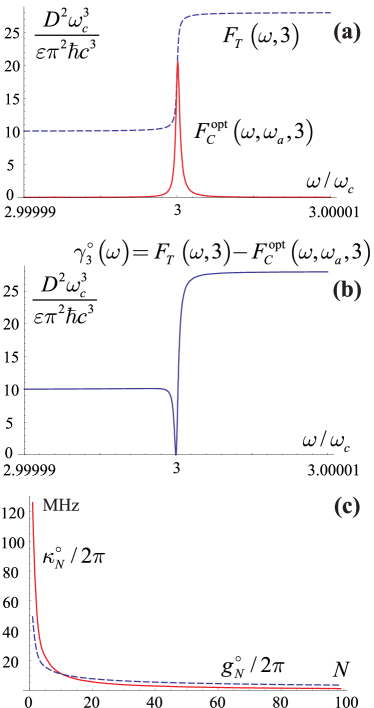
Figure 4: (Color online) (a) The cavity (solid curve) and the total (dashed curve) form-factors for $N=3$ and $f=3\,\omega_{c}$. The cavity form-factor resembles a nice Lorentzian bounded by the total form-factor. (b) The non-cavity form-factor for $N=1$ and $f=3\,\omega_{c}$. (c) Cavity-QED parameters $g^{\circ}_{N}$ and $\kappa^{\circ}_{N}$ as functions of $N$. See text for details.

The values (80) are obtained in the case when the resonator accommodates just one atomic wavelength, such that the atom is coupled to one single cavity quasi-mode, or equivalently, $\omega_{a}=\omega_{c}$ and $N=1$. We stress that the suppression of atomic decay for $\omega_{\circ}<\omega_{c}$ in a resonator accommodating just one atomic wavelength was expected, since there are no available quasi-modes below the cavity cut-off frequency to which an input pulse can couple in order to facilitate the atomic emission. We show below, however, that the inhibition of atomic emission occurs in our setup even for $\omega_{\circ}>\omega_{c}$ in a resonator that accommodates more than one atomic wavelength. This result cannot be explained by the lack of available cavity quasi-modes and constitutes a peculiar feature of the coupled atom-cavity-pulse system shown in Fig. 2(a).

In order to proceed, we consider the resonator that accommodates three atomic wavelengths, such that the atom is coupled to three quasi-modes, or equivalently, $\omega_{a}=3\,\omega_{c}$ and $N=3$. In Figs. 4(a) and (b), we display the cavity (solid curve) and non-cavity form-factors, respectively. As in the previous case, the cavity form-factor resembles a nice Lorentzian bounded by the total form-factor (dashed curve), while the atomic decay rate is suppressed inside a small window centered at $\omega=3\,\omega_{c}$. Using the atomic data (79) along with the Lorentzian (69) plotted in Fig. 4(a), we calculate $g^{\circ}_{3}$, $\kappa^{\circ}_{3}$, and $\gamma^{\circ}_{3}(\omega_{a})$, which take the values

$$\left(g_{3}^{\circ},\kappa^{\circ}_{3},\gamma^{\circ}_{3}(\omega_{a})\right)=2\pi\left(21,38,0.3\;10^{-16}\right)\text{MHz}\,.$$ (81)

If we compare these values to (80), we conclude that the cavity relaxation rate oversteps slightly the coupling strength $g_{3}^{\circ}$, while the atomic decay rate $\gamma^{\circ}_{3}(\omega_{a})$ remains negligibly small.

To reveal the dependence of $g^{\circ}$ and $\kappa^{\circ}$ on $N$, we consider the case when the resonator accommodates $N$ atomic wavelengths, that is $\ell=N\,c\,\pi/\omega_{a}$. This implies that the atom is coupled to $N$ cavity quasi-modes, such that $\omega_{a}=N\,\omega_{c}$. With this in mind, the optimal pulse

$$|\text{opt}_{N}\rangle=\sum_{\alpha}\int d\,\mathbf{k}\,\widetilde{\psi}^{\text{opt}}_{\omega_{a}}(\mathsf{k}_{z})\,\widetilde{\varphi}^{\text{opt}}_{\alpha}(\vec{k}\,,\omega_{a},N)\,b^{\dagger}_{\alpha}(\mathbf{k})|\text{vac}\rangle\,$$

penetrates the resonator, where the central frequency $\omega_{\circ}$ matches the atomic transition frequency. As before, the cavity form-factor yields a nice Lorentzian centered at $\omega=\omega_{a}$. In Fig. 4(c), we display $g^{\circ}_{N}/2\,\pi$ (dashed curve) and $\kappa^{\circ}_{N}/2\,\pi$ (solid curve) as functions of $N$, where the cavity length is bounded by $N=100$. This restriction corresponds to the length of typical macroscopic resonators used in cavity-QED experiments in the optical domain. It is clearly seen that in the region $N>10$, the cavity relaxation rate becomes slightly smaller than the respective $g^{\circ}_{N}$ parameter leading, therefore, to the atom-field evolution characterized by the inequality $g^{\circ}_{N}>\kappa^{\circ}_{N}\gg\gamma^{\circ}_{N}(\omega_{a})$. This regime ensures that the energy exchange in the coupled atom-field system develops faster than the losses due to the cavity relaxation and the atomic decay. We remark that one reason, why the curves in Fig. 4(c) drop with growing $N$, is the fact that the cut-off frequency that appears in Eqs. (63) and (77) drops with growing $\ell$, which itself is proportional to $N$.

To summarize this section, we determined the optimal lateral profile of the input pulse that ensures vanishing of the non-cavity form-factor identified with the atomic decay rate. Using the cavity form-factor associated with the optimal input pulse $|\text{opt}_{N}\rangle$, we studied the dependence of cavity-QED parameters on the cavity length that is proportional to the number of cavity quasi-modes coupled to the atom. We confirmed that the atomic decay rate becomes dramatically suppressed once the central frequency of pulse matches the atomic transition frequency. In contrast to the atomic decay for $N=1$, which is suppressed for a rather large window associated with frequency distribution $\widetilde{\psi}^{\text{opt}}(\omega)$, the respective window for $N>1$ is much smaller and, therefore, hardly accessible in practice.

IV.2 Hermite-Gaussian beam

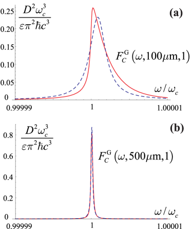
Figure 5: (Color online) The cavity form-factor (solid curve) and the associated Lorentzian (dashed curve) for $N=1$ and (a) $w=100\mu$m, (b) $w=500\mu$m. See text for details.

In the previous section, we exploited the vanishing of the atomic decay rate in order to determine the optimal input pulse $|\text{opt}_{N}\rangle$ that implies a dramatic suppression of atomic decay rate. For an appropriately large cavity length, moreover, this optimal pulse leads to an atom-field evolution with $g^{\circ}_{N}>\kappa^{\circ}_{N}\gg\gamma^{\circ}_{N}(\omega_{a})$. Although the parameter window for $N>1$, in which $\gamma^{\circ}_{N}(\omega_{a})$ becomes efficiently suppressed, is rather small to be accessible in practice, the results we obtained provide us with the relevant insights about the cavity-QED like behavior of the coupled atom-cavity-pulse system shown in Fig. 2(a).

Apparently, the lateral profile (75) has a complicated shape that makes the experimental generation of the respective spatial profile $\varphi^{\text{opt}}_{\alpha}(x,y,f,N)$ very challenging. This conclusion along with a small parameter window for $N>1$, in which the atomic decay becomes suppressed, suggest us to consider a specific input pulse that can be easily tailored in an experiment. In this section, we consider the Hermite-Gaussian beams TEM_1,0 and TEM_0,1 of the waist $w$, which we identify with the $\parallel$ and $\bot$ polarization-components of $\varphi_{\alpha}^{G}(x,y,w)$, respectively. Using these beams, we analyze the cavity-QED parameters as functions of $w$ and the number of quasi-modes coupled to the atom, $N$.

We observe that the dependence in (75) on the radial part of $\vec{k}\,$ [see Fig. 1(b)] poses the main difficulty concerning the generation of this lateral profile in practice. The dependence on the angular part of $\vec{k}\,$, in contrast, is simple and is encoded in the atom-field coupling (59)

$$\lambda_{\parallel,n}(\vec{k}\,)=\lambda_{\parallel,n}^{\circ}(k)\,\cos\vartheta\,;\quad\lambda_{\bot,n}(\vec{k}\,)=\lambda_{\bot,n}^{\circ}(k)\,\sin\vartheta\,,$$

where the dipole orientation assumption $\hat{\boldsymbol{\rho}}\cdot\hat{\mathbf{z}}=0$ and the explicit form of mode functions (18) have been used. Motivated by this simple angular dependence (preserved by the Fourier transform), we suggest the identification

$$\varphi_{\parallel}^{G}(x,y,w) = \frac{1}{\sqrt{2}}\,\mathcal{F}_{1}(x,w)\,\mathcal{F}_{0}(y,w)\quad[\text{TEM}_{1,0}]\,;$$ (82a)

$$\varphi_{\bot}^{G}(x,y,w) = \frac{1}{\sqrt{2}}\,\mathcal{F}_{0}(x,w)\,\mathcal{F}_{1}(y,w)\quad[\text{TEM}_{0,1}]\,,\qquad$$ (82b)

where

$$\mathcal{F}_{n}(z,w)=\left(\frac{2}{\pi}\right)^{\frac{1}{4}}\sqrt{\frac{1}{2^{n+\frac{1}{2}}\,n!\,w}}\,H_{n}\left(\frac{z}{w}\right)e^{-\frac{z^{2}}{2w^{2}}}\,.\quad$$ (83)

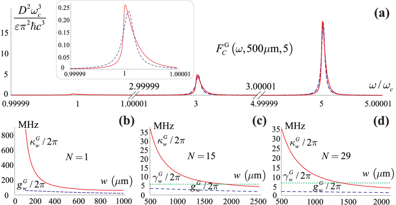
Figure 6: (Color online) (a) The cavity form-factor (solid curve) and the associated Lorentzian (dashed curve) for $N=5$ and $w=500\mu$m. The last peak resembles an almost ideal Lorentzian. (b), (c), and (d) Cavity-QED parameters $g^{G}_{w}$ (dashed curve), $\kappa^{G}_{w}$ (solid curve), and $\gamma^{G}_{w}$ (dotted curve) as functions of $w$ for $N=1$, $15$, and $29$, respectively. See text for details.

The lateral profiles (82) are the simplest and experimentally most feasible beams which exhibit the same angular dependence in physical space as the Fourier transform of $\widetilde{\varphi}^{\text{opt}}_{\alpha}(\vec{k}\,,f,N)$. These beams depend on the waist $w$ and fulfill the normalization condition (48). The corresponding input pulse, therefore, takes the form

$$|HG\rangle=\sum_{\alpha}\int d\,\mathbf{k}\,\widetilde{\psi}^{\text{opt}}_{\omega_{\circ}}(\mathsf{k}_{z})\,\widetilde{\varphi}^{G}_{\alpha}(\vec{k}\,,w)\,b^{\dagger}_{\alpha}(\mathbf{k})|\text{vac}\rangle\,,$$ (84)

where $\widetilde{\psi}^{\text{opt}}_{\omega_{\circ}}$ was defined in the previous subsection, while

$$\widetilde{\varphi}^{G}_{\alpha}(\vec{k}\,,w)=\frac{w^{2}k}{\dot{\iota}\,\sqrt{\pi}}\,e^{-\frac{w^{2}k^{2}}{2}}\left(\cos\left[\vartheta\right]\delta_{\alpha,\parallel}+\sin\left[\vartheta\right]\delta_{\alpha,\bot}\right)$$ (85)

satisfies the normalization condition (50). We insert this lateral profile into Eq. (68) and obtain

$$F^{G}_{C}(\omega,w,N)=\frac{1}{c}\left|\sum_{n,\alpha}^{N}\int d\,\vec{k}\,\,\lambda_{\alpha,n}(\vec{k}\,)\,\widetilde{\varphi}^{G}_{\alpha}(\vec{k}\,,w)\,A_{n}\left(\omega,k\right)\right|^{2},\qquad$$ (86)

which becomes after the evaluation

$$F^{G}_{C}(\omega,w,N)= \frac{\mathcal{D}^{2}\,\omega_{c}^{3}}{\epsilon\,\pi^{2}\hbar\,c^{3}}\left(\frac{\tau^{2}\,w^{4}\,\omega_{c}^{4}}{4\,\pi^{2}\,c^{4}}\right)\times$$ (87)

$$\hskip 28.45274pt\left|F^{\bullet}_{C}\left(\frac{\omega}{\omega_{c}},\frac{w\,\omega_{c}}{c},N\right)\right|^{2},$$

with the notation

$$F^{\bullet}_{C}(u,v,N)=\sum_{n}^{N}\sin\left[\frac{3\pi n}{2}\right]\times$$

$$\qquad\int_{n}^{\infty}\frac{\sqrt{s(s^{2}-n^{2})}(n+s)\,e^{-\frac{v^{2}}{2}(s^{2}-n^{2})}\,ds}{u-s-\dot{\iota}\,\tau^{2}/(4\,\pi)}\,.$$ (88)

We recall that only in the case when the cavity form-factor resembles a sharply peaked function, it plays the role of spectral mode density in a cavity-QED system with losses. We have checked that, in contrast to the optimal cavity form-factor (77), the form-factor (87) yields only deformed Lorentzians for small beam waists $w$. However, the larger the waist we consider, the less deformed the peaks we obtain. Considering the resonator that accommodates only one atomic wavelength, for instance, in Figs. 5(a) and (b) we display $F^{G}_{C}(\omega,w,1)$ (solid curves) for $w=100\mu$m and $500\mu$m, respectively, where the condition $\omega_{c}=\omega_{a}$ along with the atomic data (79) have been used. The dashed curves depict the Lorentzians obtained as the best fit to the respective solid curves. It is seen that the solid curve in Fig. 5(a) is notably deformed with regard to the dashed one, while both curves in Fig. 5(b) almost coincide.

We have checked, furthermore, that the total form-factor gives the major contribution to the atomic decay rate $\gamma^{G}_{w}(\omega)=F_{T}(\omega,1)-F^{G}_{C}(\omega,w,1)$. This leads to an efficient suppression of the atomic decay only in the region $\omega<\omega_{c}$ [see Fig. 2(c)]. Using the Lorentzians (dashed curves) from Figs. 5(a) and (b), we calculate the cavity-QED parameters

$$\left(g^{G}_{w},\kappa^{G}_{w},\gamma^{G}_{w}(0.99\,\omega_{a})\right)=2\pi\left(57,879,0.5\;10^{-4}\right)\text{MHz},\qquad$$ (89a)

$$\left(g^{G}_{w},\kappa^{G}_{w},\gamma^{G}_{w}(0.99\,\omega_{a})\right)=2\pi\left(35,89,0.5\;10^{-4}\right)\text{MHz},$$ (89b)

for the beam waists $w=100\mu$m and $500\mu$m, respectively, where the central frequency of input pulse is slightly detuned from the atomic transition frequency, that is $\omega_{\circ}=0.99\,\omega_{a}$. These parameters suggest that the cavity relaxation rate drops for a larger waist of the beam, while the atomic decay rate remains negligible if compared to other parameters. We stress, however, that a large waist $w$ of the input beam requires a large surface size of the resonator which, from an experimental point of view, is likely incompatible with a small-volume resonator that accommodates just one atomic wavelength.

Before we turn to a big-volume resonator that accommodates $N$ atomic wavelengths, we remark that, in contrast to the optimal form-factor (77) that produces a single peak at $\omega=f$, the form-factor (87) produces a series of peaks at $\omega=n\,\omega_{c}$ ($n=1,3,5,\ldots$), which resemble nice Lorentzians only for large waists $w$. To illustrate this feature, we consider the resonator that accommodates five atomic wavelengths, that is $\omega_{a}=5\,\omega_{c}$ and $N=5$. In Fig. 6(a), we display $F^{G}_{C}(\omega,500\,\mu\text{m},5)$ (solid curves) using the atomic data (79). As in the previous Figure, the dashed curves depict the Lorentzians obtained as the best fit to the respective solid curves.

It can be seen that the cavity form-factor produces three different peaks at $\omega/\omega_{c}=1,3,$ and $5$, while only the peak at $\omega=\omega_{a}$ resembles an almost perfect Lorentzian. The three Lorentzians (dashed curves) in Fig. 6(a) yield

$$\left(g^{G}_{w},\kappa^{G}_{w},\gamma^{G}_{w}(0.99\,\omega_{c})\right)=2\pi\left(2,175,0.4\;10^{-5}\right)\text{MHz}\,,\qquad$$ (90a)

$$\left(g^{G}_{w},\kappa^{G}_{w},\gamma^{G}_{w}(3.99\,\omega_{c})\right)=2\pi\left(6,68,0.8\right)\text{MHz}\,,$$ (90b)

$$\left(g^{G}_{w},\kappa^{G}_{w},\gamma^{G}_{w}(4.99\,\omega_{c})\right)=2\pi\left(10,45,4.8\right)\text{MHz}\,,$$ (90c)

corresponding to central frequencies of the input pulse which are slightly detuned from $\omega_{c}$, $3\,\omega_{c}$, and $5\,\omega_{c}$, respectively. We see that the last peak resembles not only an almost perfect Lorentzian, but also implies a higher $g^{G}_{w}$ and a smaller cavity relaxation rate $\kappa^{G}_{w}$ than those parameters associated with the other two peaks. The atomic decay rate $\gamma^{G}_{w}$, in contrast, increases due to the major contribution of the total form-factor that vanishes in the region $\omega<\omega_{c}$.

After we pointed out the main features of the cavity form-factor (87) for $N=1$ and $N=5$, let us consider a resonator that accommodates $N=1$, $15$, and $29$ atomic wavelengths and attempt to reveal the dependence of cavity-QED parameters on the beam waist $w$. Although we noticed that a large waist of the input beam is likely incompatible with a small cavity size, for completeness, we include the case $N=1$ in our considerations. From the case $N=5$ analyzed above, we learned that the form-factor produces $(N+1)/2$ peaks, such that the last peak (that matches the atomic transitions frequency) resembles the most perfect Lorentzian. Motivated by this essential requirement (that justifies our approach), we calculate below the cavity-QED parameters associated with this last peak, where the central frequency of pulse is slightly detuned from the atomic transition frequency.

In Figs. 6(b)-(d), we display $g^{G}_{w}/2\,\pi$ (dashed curve), $\kappa^{G}_{w}/2\,\pi$ (solid curve), and $\gamma^{G}_{w}/2\,\pi$ (dotted curve) as functions of $w$ for the above mentioned three values of $N$. Although in all three figures the cavity relaxation rate is efficiently suppressed for large $w$, it still remains notably higher than the atom-field coupling strength $g^{G}_{w}$. The atomic decay rate that is negligibly small for $N=1$ oversteps slightly $g^{G}_{w}$ for $N>1$, which is in agreement with the observations we already made [see (90)]. It is clearly seen, furthermore, that the atom-field evolution for $N=1$ implies $\kappa^{G}_{w}>g^{G}_{w}\gg\gamma^{G}_{w}(0.99\,\omega_{a})$. For $N>1$ and small $w$, in contrast, the atom-field evolution implies $\kappa^{G}_{w}>\gamma^{G}_{w}(0.99\,\omega_{a})>g^{G}_{w}$, while for a reasonably high $w$ the same evolution implies $\gamma^{G}_{w}(0.99\,\omega_{a})>\kappa^{G}_{w}>g^{G}_{w}$.

To summarize this section, we considered the Hermite-Gaussian input pulse (84) instead of the optimal pulse $|\text{opt}_{N}\rangle$. Using the cavity form-factor (87) associated with this (experimentally feasible) input pulse, we studied the dependence of cavity-QED parameters on the beam waist and the number of cavity quasi-modes coupled to an atom. In contrast to the results we obtained in the previous section, the atomic decay rate becomes dramatically suppressed only for $N=1$ and the central frequency that is slightly detuned from the atomic transition frequency. For $N>1$, however, the atomic decay rate becomes non-negligible and it oversteps the atom-field coupling strength, while for a reasonably large waist of the beam, the atomic decay rate oversteps both the atom-field coupling strength and the cavity relaxation rate. We conclude, therefore, that an input beam that reproduces only the angular part of the optimal lateral profile $\widetilde{\varphi}^{\text{opt}}_{\alpha}$, is insufficient to achieve the cavity-QED evolution, such that the atom-field energy exchange develops faster than the losses due to the cavity relaxation and the atomic decay.

V Summary and Outlook

In this paper, we generalized the framework of Ref. K by means of (i) an ab-initio derivation of the atom-cavity-pulse Hamiltonian, (ii) including the $\parallel$-component of light polarization, (iii) treating the cavity relaxation as a function of transmissivity and reflectivity, (iv) considering a realistic (non-averaged) atomic dipole, and by (v) analyzing the resonators which accommodate $N\geq 1$ atomic wavelengths. Using this generalized framework, we derived the cavity-QED parameters and revealed their dependence on the atom and cavity characteristics, number of cavity quasi-modes coupled to the atom, and the spatial distribution of the input pulse. The optimal spatial distribution that yields vanishing of the atomic decay rate was determined. We calculated cavity-QED parameters for this optimal distribution and found that the atomic decay is efficiently suppressed once this optimal pulse with a proper frequency distribution penetrates the resonator. We demonstrated that the suppression of atomic decay occurs even for a central frequency that is larger than the cut-off frequency in a larger resonator.

Besides this optimal pulse, the scenario in which a Hermite-Gaussian beam penetrates the resonator was considered. We discussed in detail this scenario and revealed the dependence of the cavity-QED parameters on the beam waist and the cavity length. In contrast to the results obtained for an optimal pulse, the atomic decay becomes suppressed only in a resonator that accommodates one single atomic wavelength. We concluded that an input pulse that reproduces only the angular part of the optimal spatial distribution is insufficient and so, also the radial profile has to resemble the respective profile associated with the optimal pulse.

We found that the spatial distribution of the input pulse determine the radiative properties of an atom coupled to a planar resonator. By providing the coupled atom-cavity system with an input pulse that resembles the optimal pulse or the spatial distribution that maximizes the non-cavity form-factor, therefore, one can either suppress completely the atomic decay or enhance the spontaneous emission on demand. This property suggests that our system can act as a quantum memory for long-term storage of a single qubit, where the two-level atom inserted into the resonator is interpreted as a qubit, while the (controlled) atomic decay constitutes the main source of dephasing and decoherence. Besides the storage of a qubit, a quantum memory should also provide reliable write-in and read-out mechanisms, which together with a quantitative characterization of the memory itself shall be addressed in our future works.

To conclude, we showed that our atom-cavity-pulse system can behave as a cavity-QED system exhibiting the spectral mode density of a completely (3D) confined system with losses. We remark, however, that our system is a typical 1D confined system, in which only one component of the photon field is confined, while the two remaining components propagate in free space. On the other hand, although an efficient and deterministic atom-light coupling in free space poses a serious experimental challenge apb89 ; jmo58 ; np7 , an atom-light interface in free space may open a route towards scalable quantum networking due to a moderate demand of physical resources. The remark above suggests that the studied atom-cavity-pulse system can be interpreted as a system that combines both cavity-QED and free space features. Indeed, by making the mirrors of the planar resonator completely transparent, we would (effectively) reproduce the interaction of an atom and an input pulse in free space. We stress that, although justification of the results obtained in this paper relies on the restriction $\tau\ll 1$ [see (8)], in principle, this restriction can be reasonably relaxed at the expense of introducing nonorthogonal modes in our framework pra62 .

- (1) H. Walther, B. T. H. Varcoe, B.-G. Englert, and T. Becker, Rep. Prog. Phys. 69, 1325 (2006).
- (2) J. M. Raimond, M. Brune, and S. Haroche, Rev. of Mod. Phys. 73, 565 (2001).
- (3) E. T. Jaynes and F. W. Cummings, Proc. IEEE 51, 89 (1963).
- (4) A. Boca et al., Phys. Rev. Lett. 93, 233603 (2004).
- (5) A. Blais et al., Phys. Rev. A 75, 032329 (2007).
- (6) D. Hunger et al., New J. Phys. 12, 065038 (2010).
- (7) A. V. Kavokin, J. J. Baumberg, G. Malpuech, and F. P. Laussy, Microcavities, (Oxford University Press Inc., New York, 2007).
- (8) M. Khanbekyan, L. Knöll, D. G. Welsch, A. A. Semenov, and W. Vogel, Phys. Rev. A 72, 053813 (2005).
- (9) D. Petrosyan and M. Fleischhauer, Phys. Rev. Lett. 100, 170501 (2008).
- (10) C. Y. Hu, W. J. Munro, and J. G. Rarity, Phys. Rev. B 78, 125318 (2008).
- (11) K. Koshino, S. Ishizaka, and Y. Nakamura, Phys. Rev. A 82, 010301(R) (2010).
- (12) D. Pagel, H. Fehske, J. Sperling, and W. Vogel, Phys. Rev. A 86, 052313 (2012).
- (13) R. J. Cook and P. W. Milonni, Phys. Rev. A 35, 5081 (1987).
- (14) F. De Martini, M. Marrocco, and P. Mataloni, L. Crescentini, R. Loudon, Phys. Rev. A 43, 2480 (1991).
- (15) S. M. Dutra and P. L. Knight, Phys. Rev. A 53, 3587 (1996).
- (16) B. J. Dalton, M. Babiker, P. L. Knight, Opt. Comm. 152, 36 (1998).
- (17) B. J. Dalton and P. L. Knight, J. of Mod. Opt. 46, 1817 (1999); 46, 1839 (1999).
- (18) O. Jedrkiewicz and R. Loudon, Phys. Rev. A 60, 4951 (1999).
- (19) I. Abram and J. L. Oudar, Phys. Rev. A 51, 4116 (1995).
- (20) K. Koshino, Phys. Rev. A 73, 053814 (2006).
- (21) T. B. Norris, et al., Phys. Rev. B 50, 14663 (1994).
- (22) C. Weisbuch, M. Nishioka, A. Ishikawa, and Y. Arakawa, Phys. Rev. Lett. 69, 3314 (1992).
- (23) H.-J. Briegel, W. Dür, J. I. Cirac, and P. Zoller, Phys. Rev. Lett. 81, 5932 (1998).
- (24) N. Gisin, G. Ribordy, W. Tittel, and H. Zbinden, Rev. Mod. Phys. 74, 145 (2002).
- (25) M. O. Scully and M. S. Zubairy, Quantum Optics, (Cambridge University Press, London, 1997).
- (26) C. Cohen-Tannoudji, J. Dupont-Roc, G. Grynberg, Photons and Atoms (John Wiley Sons, USA, 1997).
- (27) M. Born and E. Wolf, Principles of Optics, (Cambridge University Press, London, 1999).
- (28) S. M. Dutra, Cavity Quantum Electrodynamics, (John Wiley Sons, Inc., New Jersey, 2005).
- (29) U. Fano, Phys. Rev. 124, 1866 (1961).
- (30) S. M. Barnett and P. M. Radmore, Methods in Theoretical Quantum Optics, (Oxford University Press, New York, 1997).
- (31) S. M. Barnett and P. M. Radmore, Opt. Comm. 68, 364 (1988).
- (32) K. J. Blow, R. Loudon, S. J. D. Phoenix, and T. J. Shepherd, Phys. Rev. A 42, 4102 (1990).
- (33) M. Fox, Quantum Optics, (Oxford University Press, New York, 2006).
- (34) D. A. Steck, Cesium D line data, (Online, 2003).
- (35) M. Sondermann, et al., App. Phys. B, 89, 489 (2007).
- (36) S. A. Aljunid, et al., J. of Mod. Opt. 58, 299 (2009).
- (37) N. Piro, et al., Nat. Phys. 7, 17 (2011).
- (38) S. M. Dutra and G. Nienhuis, Phys. Rev. A 62, 063805 (2000).