Shear and rotation in Chaplygin cosmology
Abstract
We study the effect of shear and rotation on results previously obtained dealing with the application of the spherical collapse model (SCM) to generalized Chaplygin gas (gCg) dominated universes. The system is composed of baryons and gCg and the collapse is studied for different values of the parameter of the gCg. We show that the joint effect of shear and rotation is that of slowing down the collapse with respect to the simple SCM. This result is of utmost importance for the so-called unified dark matter models, since the described slow down in the growth of density perturbation can solve one of the main problems of the quoted models, namely the instability described in previous papers [e.g., H. B. Sandvik et al., Phys. Rev. D 69, 123524 (2004)] at the linear perturbation level.
pacs:
98.80.-k., 95.36.+x, 95.35.+dI Introduction
During the 1990s, numerous results showed that the cold dark matter (CDM) model approach is not sufficient to describe the observed universe. Nowadays, the scenario that best describes our Universe is a flat cosmology with dark matter (DM) and an exotic component with a negative pressure, usually named dark energy (DE). This last component is, in the new picture, the responsible of the accelerated rate of expansion of the Universe. This last conclusion, coming from the observations of high redshift supernovae, which are dimmer than expectations [1], was also confirmed by several others independent observations (e.g. the baryon acoustic oscillations [2], the angular spectrum of the CMBR temperature fluctuations [3], the integrated Sachs-Wolfe effect [4]. Nevertheless, after a decade of studies, the nature of the DE continues to remain a mystery, and as a consequence of this ”ignorance”, a large number of models have been proposed. The simplest is to identify DE with the cosmological constant , and the energy of vacuum, so obtaining the CDM model, in which the equation of state (EoS) of DE is simply given by . In order to alleviate one of the problems of the CDM model, namely the cosmological constant concordance problem, several other alternative DE models have been proposed. Extensions of this model are based on a scalar field weakly interacting with matter (quintessence models) [5], K-essence, phantom models, or unified dark matter models (UDM) (see, e.g., Ref. [6]). In UDMs, DM and DE are described by the same physical entity. One peculiar case is the so called generalized Chaplygin gas (gCg), introduced by Kamenshchik [7] and then developed in studies by [8].
The EoS describing the gCg is
| (1) |
where and are positive constants, is the density, and is the pressure. When , the gCg corresponds to the standard Chaplygin gas (sCg)111The sCg is named after Sergey A. Chaplygin, the Russian physicist who studied it in a hydrodynamical context [9].
Avelino [10] showed that the gCg background density evolution is
| (2) |
where is the cosmic scale factor, related to the cosmological redshift by , and , is the density at the present epoch.
The EoS parameter, , is given by
| (3) |
It is important to stress that Eq. (3) shows that the gCg behaves as DM at early time (), and at later ones , approaching a DE behavior.
Several theoretical [11] and observational consequences of the Chaplygin gas have been studied. Cosmological tests using CMB measurements [12], measurements of X-ray luminosity of galaxy clusters [13], SNe Ia data [14], lensing statistics [15], have been performed.
In the context of UDMs with , observations of large-scale structure [16, 17] and comparison of the linear theory with observations have put in evidence some problems of the gCg UDM. Avelino [17] studied the onset of the nonlinear regime in gCg UDMs, showing that the transition from the DM behavior to the DE one is not smooth, and showed that in gCg UDM non-linear effects generate a non trivial backreaction in the background dynamics. This implies a break down of the linear theory at late times (even on large scales), for all models. They also pointed out the need to take into account non-linear effects when comparing with cosmological observations.
However, notwithstanding the linear perturbation theory has shown that not all favor structure formation, there is a marginal degree of agreement between gCg UDM and large scale structure observations [18].
In order to have a clearer idea of the importance of the gCg as an alternative to the CDM, it is necessary to study the non-linear evolution of DM and DE in the Chaplygin gas cosmology. This was partly performed by Ref. [19]. Moreover, a fully non-linear analysis would require SPH simulations (see, e.g., Refs. [20, 21, 22, 23]). An alternative analytical approach to perform the quoted non-linear analysis and study the non-linear evolution of perturbations of DM and DE, is the popular spherical collapse model (SCM) introduced in the seminal paper of Ref. [24], extended and improved in following papers [25, 26, 27, 28, 29, 30, 31, 32].
The SCM proposed by Ref. [24] does not contain non-radial motions and angular momentum. The way to introduce angular momentum in the SCM, and its consequences, were studied in several papers [28, 33, 34, 35, 36, 29, 37, 38, 39, 31, 32, 40, 41].
Fernandes [42] used the SCM to perform the quoted non-linear analysis. Their Friedmann-Lemaître-Robertson- Walker (FLRW) universe was endowed with two components: gCg and baryons222Radiation was neglected since the study considered only the post-recombination epoch. An interesting feature of Fernandes’ treatment [42] is the fact that differently from other works (e.g., Refs. [19, 43, 44]), they considered the collapse of both gCg and baryons. Moreover, they assumed, for the background and the collapsing region, a time-dependent equation-of-state parameter , and derived a more accurate expression for the effective sound speed, , with respect to previous studies (e.g., Ref. [45]). However, their study did not consider two important factors, namely rotation (vorticity), , and shear, . Nevertheless, in any proper extension of the SCM the contraction effect produced by shear and the expansion one produced by vorticity should be considered, as done by Ref. [46]. The previous authors studied the effect of shear and vorticity only in DM-dominated universe, and only in Ref. [47] were shear and vorticity effects considered in the case of DM- and DE-dominated universes.
In the present paper, we study how the shear, , and the vorticity, , change the results obtained by Ref. [42].
II Model
As we already reported, the SCM is a surrogate to N-body simulations to study the evolution of a density perturbation in the nonlinear phase. Because of the Birkhoff theorem, a slightly overdense sphere, embedded in the Universe, behaves exactly as a closed sub-universe. In the model the overdensity is divided into mass shells, each one expanding with the Hubble flow from an initial comoving radius to a maximum one (usually named turn-around radius, ), and eventually collapse to a singularity (see Refs. [46, 48], to see how the singularity can be eliminated). Collapse to a point will never occur in practice, since dissipative physics and the process of violent relaxation will convert the kinetic energy of collapse into random motions, giving rise to a ”virialized” structure (virialization occurs at ). Once a non-linear object has formed, it will continue to attract matter in its neighborhood and its mass will grow by accretion of new material, in the process of ”secondary infall”.
In the seminal paper of Ref. [24], the authors were interested in the formulation of a theory of infall of matter into clusters of galaxies. The equations of dynamics of the structure written by them are relativistic [Eq. (7) of Ref. [24]], but they continued the treatment thinking in terms of Newtonian mechanics. Their treatment supposed that the structure collapsed radially and that non-radial motions were not present. Several following papers showed how to introduce non-radial motions, and angular momentum, , [28, 33, 34, 35, 36, 29, 37, 38, 39, 31, 32, 40] preserving spherical symmetry333Spherical symmetry is preserved if one assumes that the distribution of angular momenta of particles is random, implying a net null mean angular momentum [35].. The equations of the SCM with angular momentum can be written as (e.g., Refs. [49, 37, 40]):
| (4) |
SCM equations can be written in terms of the overdensity , using General Relativity [50] or in the Pseudo-Newtonian (PN) approach to cosmology [51]. In the PN approach, the evolution equations of in the non-linear regime has been obtained and used in the framework of the spherical and ellipsoidal collapse, and structure formation by Refs. [52, 53, 54, 55, 56].
In order to obtain the quoted equations, we assume that the fluid satisfies the equation-of-state (we assume that the velocity of light ), and we use in the calculation the generalizations of the continuity equation, of Euler’s equation (both valid for each fluid species ), and of Poisson’s equation (which is valid for the sum of all fluids) given by [51, 56]:
| (5) |
| (6) |
| (7) |
where , , and denote, respectively, the density, pressure, velocity and the Newtonian gravitational potential of the cosmic fluid.
It is important at this stage to recall that in order to derive our equations describing the evolution of perturbations, we assume the validity of the pseudo-Newtonian approach. This approach tries to include relativistic effects (like the inclusion of pressure) adding additional terms to the usual hydrodynamical equations. This is particularly evident in Eqs. (5)-(7). Relativistic contributions play a role in all the equations. Due to the equivalence principle, the pressure now acts as a source of the gravitational potential in Poisson’s equation [Eq. (7)] and modifies the denominator of the last term on the rhs of Eq. (6) (Euler equation). This set of equations is valid only for subhorizon scales and they do not take into account possible effects at scales larger than the horizon. Despite their limitations, they proved to be very useful to describe structure formation in quintessence models and their predictions were in agreement with results of N-body simulations (see for example the appendix in Ref. [44] and references therein). The equations as presented here, are not simply a generalization of Newtonian hydrodynamical equations, but they have a well defined theoretical justification. As detailed in Ref. [44], to which we refer for more details, the pseudo-Newtonian equations can be derived directly from General Relativity, assuming the stress-energy tensor of a perfect fluid characterized by density and pressure. Given the stress-energy tensor , one computes its four-divergence () and its contraction with the projection tensor . The first, contracted with the four-velocity, gives the general relativistic continuity equation, the second the Euler equation. Specifying the usual Newtonian metric and under the assumption of weak field and small velocities () we obtain the pseudo-Newtonian equations. Another confirmation of the validity of our approach is that our perturbed equations (11) and (12) coincide with the set of Eq. (30) in Ref. [57] assuming further that time derivatives of the gravitational potential are negligible with respect to spatial derivatives and that perturbations in the pressure term are not adiabatic. It might appear that there are differences between the two sets of equations, but this is due to the fact that we work in the configuration space while Ref. [57] worked in the Fourier space. Slightly different is the reasoning behind the derivation of Poisson’s equation. To derive it we can proceed in two different ways. The first one is to combine Eqs. (23a) and (23d) in Ref. [57], or work it out directly with the assumed metric.
We would like to recall that in this work, we want to generalize the work of Fernandes [42] taking into account the contribution of the shear and rotation terms. We therefore closely follow the derivation of their equations.
Introducing cosmological perturbations in the previous equations, using comoving coordinates, , using , and assuming that and are functions of time only, the equations for the perturbed quantities are:
| (8) |
| (9) |
| (10) |
where is the effective sound speed of each fluid. 444Note that in the previous equations, refers to gradient with respect to comoving coordinates .
The previous equations can be simplified as in Ref. [56],
| (11) | |||||
| (12) |
where and is the peculiar velocity field.
If we do not discard the shear and vorticity, the equations read:
| (13) | |||||
| (14) | |||||
In Eq. (11) the number of equations is equal to the number of cosmological fluid components in the system. For a ‘top-hat’ profile, resulting in , the peculiar velocity is the same for all fluids (, , ), resulting in only one Eq. (12) [or Eq. (14)]. The reason for this is that to preserve the top-hat profile, all fluids flow in the same way [58]. We remind the reader that shear and vorticity are present already in Eq. (9), via the term . To obtain and , one simply needs to take the divergence of Eq. (9).
In terms of the scale factor , and recalling that , the previous equations can be expressed in the form:
| (15) | |||||
| (16) | |||||
where the prime denotes the derivative with respect to .
The evaluation of the term was discussed in Ref. [47] by defining the ratio between the rotational and gravitational term in Eq. (4):
| (17) |
In the case of spiral galaxies like the Milky Way . Its value is larger for smaller size perturbations (dwarf galaxies size perturbations) and smaller for larger size perturbations (for galaxy clusters the ratio is of the order of ).
In order to obtain a value for similar to the one obtained by Ref. [59], we set for galactic masses (see also Ref. [60]).
Based on the above outlined argument for rotation, one may calculate the same ratio between the gravitational and the extra term appearing in Eq. (16) thereby obtaining
| (18) |
As previously told, our Eq. (18) is based on the assumption that the ratio of acceleration due to the shear/rotation term to that of the gravitational field, is constant during the collapse [Eq. (17)]. An objection to this argument could be that angular momentum, , generated by tidal torques could reduce in the collapsing phase, producing a reduction of the value of and consequently undermining the result of the calculation. This objection can be disproved as follows. As previously reported, according to the tidal torque theory, the large scale structure exerts a torque on the forming structure, with the result of imparting angular momentum on the protohalo [61, 62, 63, 64, 65, 66, 67, 68, 69, 70]. After the protostructure decouples from Hubble flow, turns around and starts to collapse, tidal torquing is made almost inefficient because the length of the lever arms are reduced (see Fig. 7 in Ref. [67]) [69, 70, 71]. Consequently, angular momentum acquisition is maximum at turn-around, and later it remains constant, since it is not lost in the collapse phase, as discussed by all the previous cited papers, and as known from the comparison of the galaxies rotation with the tidal torque theory (e.g., Refs. [69, 70, 68]). The term is the ratio of the angular momentum acquired through tidal torques (which as told remains constant after turn-around), the mass , and radius of the protostructure. While remains constant, , is decreasing in the collapse, and in the case of a collapsing sphere, its value at virialization is approximately . This produces an increase in the term . For precision’s sake, we should add that in the protostructure formation two sources of angular momentum are present: a) the angular momentum originated by tidal torques (about which we spoke till now) connected to bulk streaming motions, and b) the angular momentum originated by random tangential motions, often refereed to as “random angular momentum” [28, 35, 29, 37, 31, 32, 67, 72, 73]. Random angular momentum contribute to increase the total value of the angular momentum of the protostructure.
In the following, we will consider – corresponding to spiral galaxies similar to the Milky Way – and and , corresponding to systems in which rotation is less important.
At this point we want to stress out that combining Eqs. (15) and (16) will lead to a quite complicated second order ordinary differential equation that generalizes the usual evolution of the perturbations. To recover it, one has simply to identify with the unperturbed equation of state . It is also important to notice that our derivation is very general and it should not be considered as an expansion in the overdensity parameter. The equations obtained have very broad validity and they hold also in the case that .
The term used is the same proposed by Ref. [42], namely:
It was obtained by the quoted authors writing by using the EoS of the gCg, Eq. (1), and the relation between the densities in the background and in the collapsed region as follows:
| (20) |
recalling that the perturbed quantities and are related to their background counterparts by:
| (21) | |||||
| (22) |
and using and Eq. (1).
Eq. (LABEL:eq:cef) shows that the effective sound speed depends on the collapsed region (through ) and the background (through ). The relative to the collapsed region, namely , is given by Eq. (20) of Ref. [42]:
| (23) |
In order to study the effect of on the growth of perturbations, we solved a system of two Eqs. (15) (one for gCg and one for baryons), and one Eq. (16). We used three values of , namely (model equivalent to the CDM), and , and . As previously reported, we considered three values for , namely , 0.02, and 0.04. The initial conditions (ICs) for the system, the values of the density parameters, and Hubble constant are the same as in Ref. [42], and in agreement with recent values for the CDM [3]. As in Ref. [42], .
III Results
In our calculations, we used the same ICs for all the models. In Figs. 1(a)-1(c) [1(d)-1(f)], the solid lines represent the evolution of () in the case the term is not present (similarly to Ref. [42]), and from top to bottom in each plot the values of changes from , 0.5, 0.
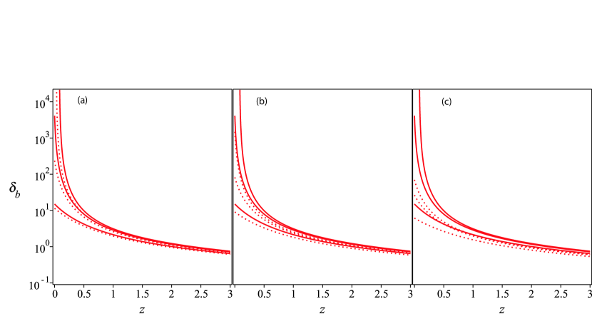
As noticed by Ref. [42], larger values of produce a faster collapse via larger values of the effective sound speed at lower . The different behaviors of () for different reflect the different evolution of and on the equations of evolution of . Moreover, at smaller – when DE dominates – larger values of produce a later transition from DM to DE dominated stages of the gCg universes.
The dotted line represents () for the same values of but when is different from zero. In Fig. 1(a) the value of is 0.01, while in Figs. 1(b) and 1(c) it is 0.02 and 0.04, respectively, and similarly for Figs. 1(d)-1(f). The effect of is that of slowing down the collapse [74], so that the collapse acceleration produced by larger values of is mitigated by the additive term. Somehow, the presence of the additive term can be mimicked by a reduction of .

Before going on, we want to stress that a comparison of our calculations with other studies, e.g., Ref. [75], in order to understand if the instability shown in our Fig 1 (when shear and vorticity are not taken into account) or their Fig. 1, is due to a term like , in their Eq. (7), is not trivial. A direct comparison of our calculations with theirs [e.g., Eq. (7)] shows that already at linear level, we obtain different equations. This is due, as said, to the different approach followed (we followed Fernandes’ approach).
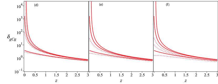
In Figs. 2(a)-2(c), we calculate using Eq. (23), and the previously calculated values of , while in Fig. 2(d), we calculate . Solid lines in Figs. 2(a)-2(d) represent when is not taken into account, for (top curve), 0.5 (median curve), 0 (bottom curve). has a strong effect on the results. Larger produce a faster collapse and a closer to zero, and moreover results in a later transition from DM to DE dominated stages of the gCg universes. The quoted result is obtained for a fixed value of ( in our case). If we increase the content of DE of the system, corresponding to increasing the value of , the collapse will happen at later times or it will be prevented with the consequence that will no longer be close to zero. The dotted lines represent the same quantity when the additive term is taken into account. In Fig. 2(a) the value of is 0.01, while in Figs. 2(b) and 2(c) it is 0.02 and 0.04, respectively. Since the effect of the additive term is to slow down the collapse, the effect on is that of showing a more pronounced departure from zero. Fig. 2(d) represents given by Eq. (3), depending on , , and , and then independent from our additive parameter, and consequently identical to Fig. 2(b) of Ref. [42]. The solid line represents the case , the dash-dotted one the case , and the dashed line the case .
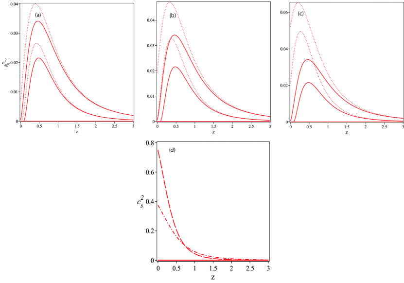
In Figs. 3(a)-(c) we plot and in Fig. 3(d) for the same values of and , and with the lines having the same meaning as in previous figures. The plot shows the different behavior of and , implying a different behavior of the gCg component locally () and in the background (). Again notice that our Fig. 3(d) for , is the same of Fig. 3(b) of Ref. [42], since the sound speed is not dependent upon the additive parameter.
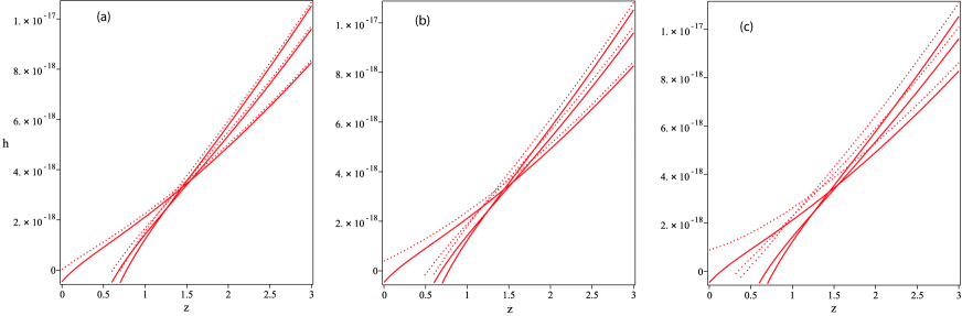
Finally, Fig. 4 plots the evolution of with . Solid lines again represent without the additive term. In each plot, has the values , 0.5, 1, from left to right. Larger values of give rise to a faster decrease in . Since the turn-around redshift, , can be defined as the at which , it is clear that higher imply a larger and an earlier collapse. Taking into account the additive term, becomes smaller with respect to the case in which it is not present. The effect of the term , is represented by the dotted lines: , , and in Figs. 4(a)-4(c), respectively.
Previous works (e.g., Refs. [75, 76]) have shown a problem in UDM models, namely oscillations or exponential blowup of the dark matter power spectrum not seen in observations – a problem which is evident on galactic scales and only at recent times, and that cannot be solved by taking baryons into account, as proposed by Ref. [77]. Both Refs. [75, 78], have shown that gravitational effects of DM, at late time, can add fluctuations to baryons but that they are unable to erase the ones already present.
Our result concerning the effect of on the growth of perturbations are partially in disagreement with the linear theory of perturbation in gCg universes (e.g., Refs. [75, 76]), and in agreement with the findings of Ref. [42]. However, in our study – due to the additive term, which has its maximum effect on galactic scales – the growth of perturbation is slowed down. This somehow implies that the additive term presence works in the direction of reducing possible present oscillations as found by Refs. [75, 76].
The previous results are perfectly framed in top-hat profiles for density and pressure. Since the profile is flat, it does not contain pressure gradients and the growth of perturbations can be suppressed only by an accelerated expansion. Assuming a nonflat initial perturbation, it would be possible to improve the understanding of how affects structure formation.
The study of the effect of pressure gradients, by using alternative profiles – such as a Gaussian profile or a Navarro-Frenk-White profile – will be the object of a future study.
Similarly to Ref. [42], we also studied how changing the ICs changes the turn-around epoch. Small changes of the ICs can produce the same turn-around redshift in all models.
IV Conclusions
In the present paper, we used the SCM to study how perturbations evolve in gCg universes, taking into account the effect of shear and rotation. We used the same as Ref. [42], and in agreement with their work we found that larger values of the parameter speed up the collapse, but the additive term produces a slowing down of this acceleration, visible in the figures showing the evolution of , (Fig. 1), , , and . The comparison of , and (the local, nonlinear parameters) with , and (the global, linear parameters) shows clear evidence of the difference in the linear and nonlinear dynamical behavior of the gCg.
Notwithstanding that the SCM is usually a faithful technique to study gravitational collapse and structure formation – with results comparable to those of simulations [79] – it would be worthwhile to check the results of this paper against SPH simulations, that would allow to take account of spatial pressure gradients. Moreover, more realistic profiles would improve our understanding of the local dynamics of gCg universes, and how the background dynamics is influenced by local non-linear inhomogeneities.
Acknowledgments: A.D.P. is partially supported by a visiting research fellowship from FAPESP (Grant No. 2011/20688-1), and also wishes to thank the Astronomy Department of São Paulo University for the facilities and hospitality. F.P. is supported by STFC Grant No. ST/H002774/1, J.F.J. is supported by FAPESP Grant No. 2010/05416-2, and J.A.S.L. is also partially supported by CNPq and FAPESP under Grants No. 304792/2003-9 and No. 04/13668-0.
References
- [1] A. Riess et al., Astron. J. 116, 1009 (1998); S. Perlmutter et al., Nature 391, 51 (1998); M. Kowalski et al., Astrophys. J. 686, 749 (2008); R. Amanullah et al., Astrophys. J. 716, 712 (2010); J. L. Tonry et al., Astrophys. J. 594, 1 (2003).
- [2] M. Tegmark et al., Astrophys. J. 606, 702 (2004); M. Tegmark et al., Phys. Rev. D 69, 103501 (2004); W. J. Percival et al., Mon. Not. R. Astron. Soc. 401, 2148 (2010).
- [3] E. Komatsu et al., Astrophys. J. 192, 18 (2011); S. W. Allen, A. E. Evrard and A. B. Mantz, Annu. Rev. Astron. Astrophys. 49, 409 (2011).
- [4] S. Ho et al., Phys. Rev. D 78, 043519 (2008).
- [5] B. Gumjudpai et al., J. Cosmol. Astropart. Phys. 6 (2005) 007; E. J. Copeland, M. Sami, and S. Tsujikawa, Int. J. Mod. Phys. D 15, 1753 (2006).
- [6] P. P. Avelino, L. M. G. Bec a, and C. J. A. P. Martins, Phys. Rev. D 77, 063515 (2008); D. Bertacca, N. Bartolo, and S. Matarrese, Adv. Astron. 2010, 904379 (2010).
- [7] A. Kamenshchik, U. Moschella, and V. Pasquier, Phys. Lett. B 511, 265 (2001).
- [8] N. Bilic , G. B. Tupper, and R. D. Viollier, Phys. Lett. B 535, 17 (2002); M. C. Bento, O. Bertolami, and A. A. Sen, Phys. Rev. D 66, 043507 (2002); V. Gorini, A. Kamenshchik, and U. Moschella, Phys. Rev. D 67, 063509 (2003).
- [9] S. Chaplygin, Sci. Mem. Moscow Univ. Math. Phys. 21, 1 (1902).
- [10] P. P. Avelino et al., Phys. Rev. D 67, 023511 (2003).
- [11] M. Bordemann and J. Hoppe, Phys. Lett. B 317, 315 (1993); J. Hoppe, preprint (hep-th/9311059) (1993); R. Jackiw, A Particle Field Theorist s Lectures on Supersymmetric, Non-Abelian Fluid Mechanics and d-Branes (MIT-CTP 3000, Cambridge: MIT) (2000); P. F. Gonza lez-Di az, Phys. Rev. D 68, 021303 (2003a); P. F. Gonza lez-Di az, Phys. Lett. B 562, 1 (2003b); G. M. Kremer, Gen. Relativ. Gravit. 35, 1459 (2003); I. M. Khalatnikov, Phys. Lett. B 563, 123 (2003); A. B. Balakin et al., New J. Phys. 5, 85 (2003); N. Bilic , G. B. Tupper, and R. D. Viollier, Phys. Lett. B 535, 17 (2002).
- [12] M. C. Bento, O. Bertolami, and A. A. Sen, Phys. Rev. D 66, 043507 (2002); M. C. Bento, O. Bertolami, and A. A. Sen, Phys. Rev. D 67, 063003 (2003a); M. C. Bento, O. Bertolami, and A. A. Sen, Phys. Lett. B 575, 172 (2003b); M. C. Bento, O. Bertolami, and A. A. Sen, Gen. Relativ. Gravit. 35, 2063 (2003c); D. Carturan and F. Finelli, Phys. Rev. D 68, 103501 (2003); L. Amendola et al., J. Cosmol. Astropart. Phys. 07 (2003) 005.
- [13] J. V. Cunha, J. S. Alcaniz, and J. A. S. Lima, Phys. Rev. D 69, 083501 (2004); Z.-H. Zhu, M.-K. Fujimoto, and X.-T. He, Astrophys. J. 603, 365 (2004).
- [14] J. C. Fabris, S. V. B. Goncalves, and R. de Sa Ribeiro, Gen. Relativ. Gravit. 36, 211 (2004); R. Colistete, Jr. et al., Int. J. Mod. Phys. D 13, 669 (2004); P. P. Avelino et al., Phys. Rev. D 67, 023511 (2003b); M. Makler, S. Q. de Oliveira, and I. Waga, Phys. Lett. B 555, 1 (2003); O. Bertolami et al., Mon. Not. R. Astron. Soc. 353, 329 (2004).
- [15] A. Dev, J. S. Alcaniz, and D. Jain, Phys. Rev. D 67, 023515 (2003); A. Dev, D. Jain, and J. S. Alcaniz, Astron. Astrophys. 417, 847 (2004); P. T. Silva and O. Bertolami, Astrophys. J. 599, 829 (2003).
- [16] T. Multama ki, M. Manera, and E. Gaztanaga, Phys. Rev. D 69, 023004 (2004); N. Bilic et al., J. Cosmol. Astropart. Phys. 11 (2004) 008; L. M. G. Beça et al., Phys. Rev. D 67, 101301 (2003); R. Bean and O. Dore, Phys. Rev. D 68, 023515 (2003).
- [17] P. P. Avelino et al., Phys. Rev. D 69, 041301 (2004).
- [18] L. M. Bec a et al., Phys. Rev. D 67, 101301 (2003); H. B. Sandvik et al., Phys. Rev. D 69, 123524 (2004); P. P. Avelino et al., Phys. Rev. D 69, 041301 (2004); V. Gorini et al., J. Cosmol. Astropart. Phys. 2 (2008) 016.
- [19] N. Bilic et al., J. Cosmol. Astropart. Phys. 11 (2004) 008.
- [20] A. V. Maccio‘ et al., Phys. Rev. D 69, 123516 (2004).
- [21] N. Aghanim, A. C. da Silva, and N. J. Nunes, Astron. Astrophys. 496, 637 (2009).
- [22] M. Baldi et al., Mon. Not. R. Astron. Soc. 403, 1684 (2010).
- [23] B. Li, D. F. Mota, and J. D. Barrow, Astrophys. J. 728, 109 (2011).
- [24] J. E. Gunn and J. R. Gott, Astrophys. J. 176, 1 (1972)
- [25] J. A. Fillmore and P. Goldreich, Astrophys. J. 281, 1 (1984).
- [26] E. Bertschinger, Astrophys. J. Suppl. Ser. 58, 39 (1985).
- [27] Y. Hoffman, J. Shaham, Astrophys. J. 297, 16 (1985).
- [28] B. S. Ryden and J. E. Gunn, Astrophys. J. 318, 15 (1987).
- [29] V. Avila-Reese, C. Firmani, and X. Hern andez, Astrophys. J. 505, 37 (1998).
- [30] K. Subramanian, R. Cen and J. P. Ostriker, Astrophys. J. 538, 528 (2000).
- [31] Y. Ascasibar et al., Mon. Not. R. Astron. Soc. 352, 1109 (2004).
- [32] L. L. R. Williams, A. Babul and J. J. Dalcanton, Astrophys. J. 604, 18 (2004).
- [33] A. V. Gurevich and K. P. Zybin, Zhurnal Eksperimental noi i Teoreticheskoi Fiziki 94, 3 ( 1988).
- [34] A. V. Gurevich and K. P. Zybin, Zhurnal Eksperimental noi i Teoreticheskoi Fiziki 94, 5 (1988).
- [35] S. D. M. White and D. Zaritsky, Astrophys. J. 394, 1 (1992).
- [36] P. Sikivie, I. I. Tkachev and Y. Wang, Phys. Rev. D. 56, 1863 (1997).
- [37] A. Nusser, Mon. Not. R. Astron. Soc. 325, 1397 (2001).
- [38] N. Hiotelis, Astron. Astrophys. 382, 84 (2002).
- [39] M. Le Delliou and R. N. Henriksen, Astron. Astrophys. 408, 27 (2003).
- [40] P. Zukin and E. Bertschinger, Phys. Rev. D 82, 104044 (2010).
- [41] A. Del Popolo and M. Gambera, Astron. Astrophys. 357, 809 (2000); 337, 96 (1998).
- [42] R. A. A. Fernandes et al., Phys. Rev. D. 85, 083501 (2012).
- [43] T. Multama ki, M. Manera, and E. Gaztan aga, Phys. Rev. D 69, 023004 (2004).
- [44] F. Pace, J. Waizmann, and M. Bartelmann, Mon. Not. R. Astron. Soc. 406, 1865 (2010).
- [45] L. R. Abramo et al., Phys. Rev. D 77, 067301 (2008).
- [46] S. Engineer, N. Kanekar, T. Padmanabhan, Mon. Not. R. Astron. Soc. 314, 279 (2000).
- [47] A. Del Popolo, F. Pace, J. A. S. Lima, IJMPD, submitted (2012), arXiv:1207.5789
- [48] D. J. Shaw and D. F. Mota, Astrophys. J. 174, 277 (2008).
- [49] P. J. E. Peebles, Principles of Physical Cosmology, Princeton University Press (1993).
- [50] E. Gaztanaga and J. A. Lobo, Astrophys. J. 548, 47 (2001).
- [51] J. A. S. Lima, V. Zanchin, and R. H. Brandenberger, Mon. Not. R. Astron. Soc. 291, L1 (1997).
- [52] F. Bernardeau, Astrophys. J. 433, 1 (1994).
- [53] T. Padmanabhan, Cosmology and Astrophysics through Problems (1996).
- [54] Y. Ohta, I. Kayo and A. Taruya, Astrophys. J. 589, 1 (2003).
- [55] Y. Ohta, I. Kayo, A. Taruya, Astrophys. J. 608, 647 (2004).
- [56] L. R. Abramo et al., J. Cosmol. Astropart. Phys. 11 (2007) 12.
- [57] C-P., Ma, & E. Bertschinger Astrophys. J. 455, 7, (1995).
- [58] L. R. Abramo et al., Phys. Rev. D 79, 023516 (2009).
- [59] R. K. Sheth, H. J. Mo, and G. Tormen, Mon. Not. R. Astron. Soc. 323, 1 (2001). See also, A. Del Popolo and M. Gambera, Astron. and Astrophys. 344, 17 (1999)
- [60] A. Del Popolo, F. Pace, J. A. S. Lima, arXiv:1212.5092.
- [61] F. Hoyle, in IAU and International Union of Theorethical and Applied Mechanics Symposium, Problems of Cosmological Aerodynamics, ed. J. M. Burger & H. C. van der Hulst (Ohio: IAU), 195 (1949)
- [62] D. W. Sciama, Mon. Not. R. Astron. Soc. 115, 3 (1955)
- [63] P. J. E. Peebles, Astrophys. J. 155, 393 (1969)
- [64] A. G. Doroshkevich, Astrophysics, 6, 320 (1970)
- [65] S. D. M. White, 1984, Astrophys. J. 286, 38 (1984)
- [66] P. S. Wesson, Astronom. Astrophys., 151, 105 (1985)
- [67] B. S. Ryden, Astrophys. J. 329, 589, (1988)
- [68] D. J. Eisenstein, & A. Loeb, Astrophys. J. 439, 250 (1995)
- [69] P. Catelan & T. Theuns, Mon. Not. R. Astron. Soc. 282, 436, (1996)
- [70] P. Catelan & T. Theuns, Mon. Not. R. Astron. Soc. 282, 455, (1996)
- [71] B. M. Schäfer arXiv 0808.0203 (2008)
- [72] A. Del Popolo, Astrophys. J. 698, 2093 (2009)
- [73] A. Del Popolo and P. Kroupa, Astron. Astrophys. 502, 733 (2009).
- [74] A. Del Popolo, Mon. Not. R. Astron. Soc. 336, 81 (2002).
- [75] H. B. Sandvik et al., Phys. Rev. D 69, 123524 (2004).
- [76] V. Gorini, A. Kamenshchik, and U. Moschella, Phys. Rev. D 67, 063509 (2003).
- [77] R. Colistete, Jr. et al., Int. J. Mod. Phys. D 13, 669 (2004).
- [78] L. M. G. Beca et al., Phys. Rev. D 67, 101301 R! (2003).
- [79] Y. Ascasibar, Y. Hoffman, and S. Gottl ober, Mon. Not. R. Astron. Soc. 376, 393 (2007).