The Role of Magnetic Fields in Transient Seismic Emission Driven by Atmospheric Heating in Flares

Abstract

Fifteen years after its discovery, the physics of transient seismic emission in flares remains largely mysterious. An early hypothesis by its discoverers proposed that these “sunquakes” are the signature of a shock driven by “thick-target heating” of the flaring chromosphere. H-$\alpha$ observations show evidence for such a shock in the low chromosphere during a flare. However, simulations of shocks driven by impulsive chromospheric heating show withering radiative losses as the shock proceeds downward. The compression of the shocked gas not only heats it but increases its density, making it more radiative. So, radiative losses increase radically with the strength of the shock. This has introduced doubt that sufficient energy from such a shock can penetrate into the solar interior to match that indicated by the helioseismic signatures. The purpose of this paper is to point out that simulations of acoustic transients driven by impulsive heating have yet to account for magnetic fields characteristic of transient-seismic-source environments. We show this to be a critically important factor that has a major impact on the seismic flux conducted into the solar interior. A strong horizontal magnetic field, for example, greatly increases the compressional modulus of the chromospheric medium. This greatly reduces compression of the gas, hence the radiative losses as the transient passes through it. This could explain the strong affinity of seismic sources to regions of strong, highly inclined penumbral magnetic fields, including the neutral lines separating opposing polarities in $\delta$-configuration sunspots. The basic point, then, is that the role of inclined magnetic fields is fundamental to our understanding of the role of impulsive heating in transient seismic emission. Obliquely inclined magnetic fields will complicate simulations of impulsive heating considerably. However, horizontal magnetic fields, as a preliminary control simulation, can be incorporated into standard 1-D thick-target-heating simulations with a relatively simple adaptation of existing HD codes.

1 Introduction

S-Introduction

The first known instance of seismic transient emission, also known as a “sunquake,” was that discovered by Kosovichev98, emanating from the X2.6-class flare of 1996 July 9 in the declining phase of Cycle 22. Seven years passed, with some major acoustically quiet flares, before Donea05 found seismic emission from multiple sources in the flares of 2003 October 28–29. This led to the subsequent discovery of about a dozen instances of transient seismic emission in the declining phase of Cycle 23, some associated with relatively weak flares. Transient seismic emission is now known to be a moderately common phenomenon. Nevertheless, something about the mechanics behind this phenomenon continues to elude us.

The significant manifestation of transient seismic emission is a pattern of outgoing ripples seen in Doppler-helioseismic observations 15–45 min following the impulsive phase of a flare. Computational seismic holography applied by Donea99, Donea05 and others, showed compact sources up to $\sim$12 Mm across at sites of hard X-ray emission, and sometimes $\gamma$-ray emission. Estimates of the seismic energy, $E_{S}$, emitted by a single compact source, based upon signatures derived from seismic holography [Donea, Braun, and Lindsey (1999), Donea and Lindsey (2005)], are frequently in the range 10²⁷–10²⁸ erg. The vertical momentum carried by a seismic transient at the solar surface is estimated at $E_{S}/c$, where $c$ is the sound speed. Taking $c$ to be $\sim$10 km s^-1 renders seismic momenta in the range 10²²–10²³ dyne s.

In large flares, there may be more than one such source, in which case the total seismic energy emitted can be correspondingly greater. This acoustic energy is only a small fraction of the total energy [Emslie et al. (2012)] estimated for a flare, generally a fraction of a percent, and for large flares often less than 10^-4 of the total.

Attempts to understand transient seismic emission have focused upon three mechanisms:

1.1 Impulsive Heating of the Chromosphere

S-TTH

Kosovichev98 attributed transient seismic emission to a pressure wave driven by “thick-target heating” of the chromosphere by energetic electrons. A good deal of what we understood of this mechanism at the time came out of 1-D numerical HD simulations (Fisher, Canfield and McClymont 1985a,b,c, thenceforth FCM) applied to pre-flare models of plage chromospheres and coronae. Energetic electrons accelerated in the corona heat the upper chromosphere to something like coronal temperatures. The initial pressure of the medium, 10–100 dyne cm^-2 is increased by about two orders of magnitude. The resulting increase in pressure drives a shock downward into the medium beneath the heated layer, carrying a momentum of the order of $10^{22}$ erg cm s^-1 (Kosovichev95). This is essentially balanced by the upward momentum of the heated layer, which explodes upward into the pre-flare corona. Zarro89 found this shock model consistent with H-$\alpha$ emission spectra typical of M-class flares.

More recent consideration to the role of impulsive chromospheric heating in transient seismic emission is given by Zharkova08 and Zharkov11.

The hypothesis that transient seismic emission is driven by impulsive chromospheric heating has the problem that severe radiative losses deplete the transient as it passes through the underlying low chromosphere. These concerns were first communicated to us by Fisher (2006, private communication). They are mentioned by Hudson08 and treated in further detail by Fisher12. This conclusion is reinforced by FCM-style simulations by Allred05, and, with improved treatment of radiative transfer, by Allred (private communication, 2012). Even in acoustically active flares the signature of heating is often evident in regions from which no seismic emission appears to emanate. This includes acoustically inactive flares, from which no transient seismic emission at all is evident.

Our understanding of the dynamics and geometry of atmospheric heating has changed dramatically since FCM. The magnetic structure of penumbrae, from which transient seismic emission generally appears to emanate, is highly filamentary, as opposed to the plane-parallel models of FCM. Fletcher08 suggest that the high-energy electrons that serve as the primary agent for the evident heating could be accelerated much deeper than in the models of FCM, i.e., in the chromosphere instead of the corona. Indeed, recent SDO/STEREO/RHSSI observations by Martinez12 using parallax to determine the source heights of white light (WL) and hard X-ray (HXR) emission associated with atmospheric heating indicate that this heating is significantly deeper than in the models of FCM.

1.2 Backwarming of the Photosphere

S-BW

Based upon some of these developments, Donea99 and Moradi07 proposed that heating of the photosphere by visible and near-UV continuum radiation from the heated chromosphere could drive a seismic transient (see also Lindsey08). In this model, a pressure transient is launched at the base of the photosphere, which most efficiently absorbs the continuum radiation from the chromosphere, and proceeds downward (and upward) from thence. Once the downward component of the transient penetrates into the solar interior, further radiative losses are blocked by the high opacity of ionized hydrogen. This mechanism, known as “backwarming,” was suggested by sources of seismic transient emission that coincided closely with transient white-light flare kernels (Lindsey08).

Instances have since been discovered of strong seismic emission from regions that show no appreciable excess in visible continuum radiation integrated over the neighborhood of the seismic source. An example is the X2.2-class flare on 2011 February 15. Integrated over a circular disk whose area is 90 Mm², encompassing the seismic source, these fluctuations are only 0.12% of the quiet-Sun intensity. For comparison, a similar average taken over the seismic source of the white-light flare of 2003 October 29 found a continuum emission 10% in excess of the quiet-Sun intensity [Donea and Lindsey (2005)], i.e., about 80 times greater than in the flare SOL2011-02-15 [Alvarado Gómez et al. (2012)]. According to our rough understanding of how back-warming could prospectively work as a seismic source [Lindsey and Donea (2008)], a compression wave driven by heating commensurate with this degree of fluctuation in continuum intensity could explain barely 2% of the the seismic energy that appears to emanate from the flare SOL2011-02-15. Because of this, it is evident that some other mechanism must be in operation to explain the seismic transient released by this flare.

Variations to the back-warming theme draw upon energetic protons [Zharkova (2008)]. Protons with energies of 200 MeV could penetrate to the base of the photosphere, heating it directly. Protons of these energies interact with the nuclei of elements such as oxygen, iron and magnesium [Najita and Orrall (1970)] to excite $\gamma$ rays. Such $\gamma$ rays are indeed observed in some seismically active flares. However, we now know of instances (Donea06) of strong seismic emission from flares from which no $\gamma$ radiation was detected.

1.3 Lorentz-Force Transients

S-LFT

Based largely upon the foregoing assessments, Hudson08 and Fisher12 proposed that transient seismic emission is the result of Lorentz-force transients, caused by the sudden re-configuration of the magnetic field in the impulsive phase of the flare.

Magnetic signatures roughly consistent with Lorentz-force transients driving transient seismic emission consistent with helioseismic signatures are reported by Donea06, Sudol05, Wang02 Wang10, Petrie10, Petrie12 and others. These signatures appear to be encumbered by two significant qualifications:

• Magnetic signatures representing highly perturbed radiative environments such as are typical of flares are notoriously unreliable, often showing momentary reversals in the field direction inconsistent with expectations based upon MHD in a highly conducting medium.

• Such magnetic signatures are common in acoustically inactive flares, as they are in acoustically active flares in wide-spread regions from which no detectable seismic emission emanates.

A-G12 studied the seismically active flare SOL2011-02-15, concentrating on the magnetic signature in the source region of the strongest of two sources (Figure 1). Based upon line-of-sight magnetic signatures immediately before the impulsive phase and 10–15 minutes after, they offer a somewhat discouraging appraisal of the potential of the local Lorentz force transient as a driver for the seismic emission observed. However, they do not rule it out. Further consideration to the role of Lorentz-force transients in this flare is given by Zharkov11, based largely upon the apparent magnetic connectivity between the primary acoustic source and a second one, which they themselves discovered.

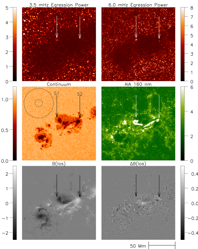
Figure 1.: Doppler egression-power maps from SDO/HMI observations representing 1-mHz bandpasses centered at 3 mHz (upper left) and 6 mHz (upper right) in units of m² s^-2. Middle row shows a pre-flare HMI continuum intensity snapshot (left) and an AIA snapshot (right) of 160 nm continuum radiation in the early impulsive phase, both normalized to unity for the quiet Sun. Bottom row shows a pre-flare HMI line-of-sight magnetogram (left), and line-of-sight difference in the magnetic field from before to after the impulsive phase, the time difference being 15 min, both in units of kGauss. Arrows locate compact sources of seismic emission in the upper right egression-power map. Concentric circles in the upper left frame show the dimensions of the pupil applied in the helioseismic egression computations in the top row.F-eg-pwr-maps

AIA observations show strong 160 nm emission from the end of a ribbon $\sim$2.8 Mm SSE of the seismic source in the early impulsive phase (middle-right panel of Figure 1). Within seconds, emission in this region is obscured by saturation/overflow from strong, extended emission at large. Hinode/SOT observations in the CaII K-line show a very similar ribbon that sweeps northward through the acoustic source region in the minute or so following the time of the 160 nm snapshot. This suggests strong heating of the chromosphere, that might drive a seismic transient—if the resulting shock could somehow escape the radiative losses described in §S-TTH, above. A-G12 report HXR emission whose RHESSI signature encompasses the seismic source region, which would connect the heat source to energetic electrons. Like the magnetic signatures, both the 160-nm and the HXR sources are stronger in other far-removed regions, from which no seismic emission is detected.

2 Regional Selectivity

S-Selectivity

In summary, then, the signatures indicating impulsive chromospheric heating and Lorentz-force transients appear to share one conspicuous quality in common, both in the flare SOL2011-02-15 and in other flares, acoustically active or not: They all show strong, apparently transient signatures in vast regions from which no significant seismic emission emanates. It appears that there has to be something special about seismic-source regions such that any of the mechanisms yet considered (or perhaps others) could have a role in transient seismic emission. For either chromospheric heating or Lorentz-force transients to satisfy the helioseismic signatures, something distinctive about their respective operations begs to be identified that makes it horizontally selective of the highly restrictive regions from which seismic radiation emanates. This is the primary theme of this study. Failing such an identification, it should begin to appear that seismic transient emission must depend upon some mechanism not yet considered.

In the case of Lorentz-force transients, for example, a basis for “regional selectivity” might be the difficulty of credible magnetic measurements during the impulsive phases of flares. If transient magnetic signatures during the impulsive phase of the flare are simply spurious, then magnetic variations that actually occur in the impulsive phase may be insufficiently sudden to excite a seismic transient—except where the signatures of transient seismic sources actually appear. Magnetography is known to be highly susceptible to this liability under flaring conditions. If this is the basis of the regional selectivity we find, then what is distinctive about seismic source regions so that magnetic transients in them are more sudden than elsewhere?

For transients driven by impulsive heating, a highly suggestive basis for regional selectivity is the impact of a strong magnetic field on the overbearing radiative losses discussed in §1.1, which discourage the downward conduction of seismic transients in non-magnetic simulations. In the absence of a magnetic field, a shock driven by the expansion of the heated medium compresses the underlying medium, heating it and increasing its density. Both the heating and the increased density make the gas a more effective radiator. Hence, the radiative losses increase strongly, nonlinearly, with the degree of compression, which is 1–2 orders of magnitude in the low chromosphere in the simulations of Fisher, Canfield & McClymont (1985a,b,c). The onus appears to be whether any amount of impulsive heating can manifest a seismic transient that can survive the radiative losses entailed in passage through both the low chromosphere and photosphere to penetrate into the solar interior.

As a screening measure to judge whether impulsive heating merits serious consideration, simulations such as those of Fisher12 and Allred05 can seem discouraging indeed. However, we want to point out just the opposite, that these simulations are entirely consistent with helioseismic signatures as we know them. Impulsive chromospheric heating simulations to date have been computed only for non-magnetic media, from which detectable transient seismic emission has indeed never emanated, to our knowledge. Based upon this, we propose, as a hypothesis, that the very radiative losses that discourage the impulsive heating as a driver of transient seismic emission in the context of a non-magnetic medium are the key to the high degree of regional selectivity shown by transient seismic emission in flares. Essentially all transient seismic sources appear in sunspot penumbrae, regions known to be infused with strong, highly inclined magnetic fields. We want to propose that a major mechanical role of this field can be a radical reduction in radiative losses in those localities. This reduction in radiative losses could rescue impulsive heating as a tenable source of the seismic emission that emanates from some flares. Moreover, if backed up by appropriate MHD simulations that incorporate oblique magnetic fields, and by appropriate observational diagnostics, it may very well explain the high regional selectivity that characterizes transient seismic sources.

3 The Mechanical Role of an Inclined Magnetic Field in Seismic-Transient Conduction

S-mechanics

For a rough, preliminary understanding of the role of an inclined field, we consider the simplest case, that of a horizontally uniform medium infused with a horizontal field, likewise horizontally uniform, into which we introduce a horizontally uniform shock, driven by a horizontally uniform thick-target-profile heating. In the MHD context the action of the horizontal magnetic field is essentially equivalent to that of a large increase in the compressional modulus of the medium, the magnetic component of which is

$$\kappa_{M}~{}=~{}-V{\partial p_{M}\over\partial V}~{}=~{}2p_{M},\ilabel{eq-mag-mod}$$ (1)

where

$$p_{M}\equiv{B^{2}\over 8\pi}\ilabel{eq-mag-pressure}$$ (2)

is the magnetic pressure, with $B$ the magnetic field strength, and $V$ represents the volume of the local unit of medium being vertically compressed by the shock. The compression, then, is perpendicular to $\bf B$, the local magnetic induction. For a magnetic field of 500 Gauss in the primary source region of the flare SOLA2011-02-15, this is $\sim$40 times the isothermal gas modulus,

$$\kappa_{g}~{}=~{}-V\Big{(}{\partial p_{g}\over\partial V}\Big{)}_{T}~{}=~{}p_{g},\ilabel{eq-gas-mod}$$ (3)

where $p_{g}$ is the local gas pressure.

The presence of a horizontal magnetic field whose strength is typical of sunspot penumbrae, then, will make the medium much more “vertically rigid,” i.e., much more resistant to compression perpendicular to the field. The medium will therefore conduct seismic energy downward with a much smaller degree of compression. The radiative losses will be reduced accordingly. Since the radiative losses in the non-magnetic medium increase strongly, i.e., highly non-linearly, with compression, we have to suspect that the radiative losses will be a small fraction of those indicated by the non-magnetic simulations, for a sufficiently inclined field. This will introduce a high degree of selectivity towards regions of highly inclined magnetic field. In the ideal case of a horizontal field conducting a downwardly propagating transient, nearly all of the compressional work will be done on the magnetic field, which is almost completely elastic, hence lossless.

The role of inclined magnetic fields, then, needs to be seriously considered as a prospective explanation of strong regional selectivity of transient seismic sources in favor of strongly inclined magnetic fields. Indeed, among the most conspicuous such source regions is the penumbral neutral line separating umbrae of opposing polarities in $\delta$-configuration sunspots. In these instances, e.g., Moradi07 (see Figure 2 of this study), the magnetic field is exceptionally strong, leading to an especially high magnetic modulus, $k_{M}$, and is essentially horizontal, hence avoiding losses due to coupling between fast and slow modes (see Cally11).

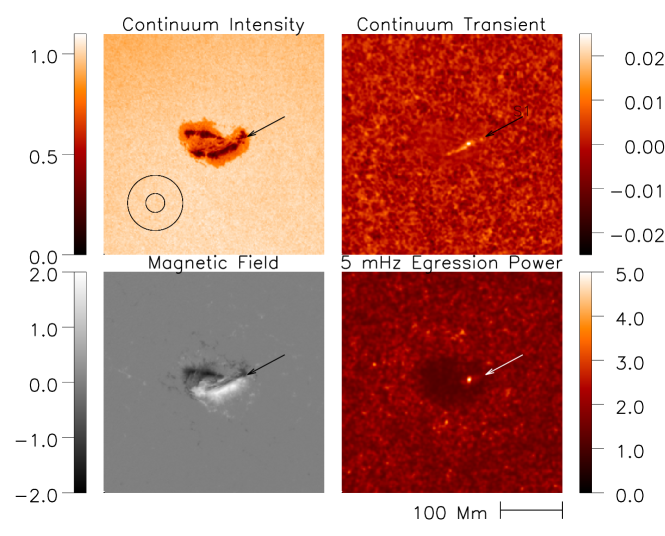
Figure 2.: Doppler egression-power map (lower right) of seismic emission from NOAA AR10720 at 00:42 UT, during the impulsive phase of the flare of 2005 January 15. The line-of-sight magnetogram (lower left) identifies AR10720 as a $\delta$-configuration sunspot. Upper left frame shows the pre-flare continuum intensity, from SOHO/MDI. Upper right frame shows the continuum-intensity excess in the impulsive phase of the flare, from GONG. Bottom left frame shows a line-of-sight magnetogram shortly before flare onset. Concentric circles in the upper left frame show the dimensions of the pupil applied in the helioseismic egression computation.fig-delta-spot

4 Qualifications

S-qualifications

4.1 Magnetic Encumbrance of the Work Capacity of a Heated Gas

S-mag-encumberance

Somewhat anticipating realistic simulations, it should be noted that the magnetic rigidity that should (we propose) so greatly reduce radiative losses once a transient has development must also inhibit this development. This is because it encumbers the expansion of the heated medium, which is the agent of mechanical work upon its surroundings. Heating applied to a low-$\beta$, i.e. magnetically rigid, medium will respond with less expansion than a non-magnetic medium. At some point this will limit the capacity of the heated gas to do work on its surroundings, including on the magnetic field itself, hence the efficiency with which impulsive heating will drive a seismic transient. For an estimate of this encumbrance over a range of temperatures to which the gas can be heated, we determine the “mechanical work capacity” with and without a magnetic field for a unit mass (1 gram) of hydrogen, with a helium abundance of 10%, initially at temperature $T_{0}$ of 4,000 K and under a gas pressure, $p_{g0}$, of 500 dyne cm^-2. The gas is first heated at constant volume, $V_{0}$, to a temperature $T_{0}~{}+~{}\Delta T$, raising its pressure as illustrated by the vertical displacements in the $p$-$V$ trajectories plotted in Figure 3. In this representation, the non-magnetic gas is represented by the blue locus. The green locus represents an identical gas with a horizontal magnetic field initially of 500 Gauss. Once heated, these gas samples are expanded vertically and adiabatically to their original pressures, and subsequently allowed to cool at the original pressure to the original temperature of 4,000 K. We recognize the areas of the respective closed curves in the $p$-$V$ plane as the respective adiabatic work capacities,

$$\Delta W~{}=~{}\oint_{\cal R}pdV,\ilabel{work}$$ (4)

of the heated gas samples.

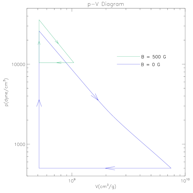
Figure 3.: Trajectories in $p$–$V$ space of a unit mass (1 g) of chromospheric hydrogen-helium initially at a temperature $T$ of 4,000 K and pressure of 500 dyne cm^-3 heated to 10⁵ K, then expanded adiabatically to the initial pre-heated pressure, and finally cooled at that pressure. The blue locus represents a non-magnetic medium. The green locus represents the same cycle for a medium infused with a 500-Gauss magnetic field. We recognize the respective “adiabatic work capacities,” $\Delta W$, of these cycle to be the area in $p$–$V$-space enclosed by the respective curves. For the foregoing parameters, $\Delta W$ is 1.44$\times$10¹³ erg g^-1 for the non-magnetic medium and 0.459$\times$10¹³ erg g^-1 the magnetic medium.

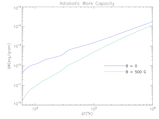
Figure 4.: Mechanical work capacity of an unmagnetized heated gas (blue) is compared with the same for a gas infused with a horizontal magnetic field whose initial strength is 500 Gauss is plotted as a function of the temperature increase, $\Delta T=T_{1}~{}-~{}T_{0}$, in the heated gas. The gas, in thermal equilibrium with a helium abundance of 10%, is heated at constant volume from an initial temperature of 4,000 K to the temperature indicated by the abscissa. It is then expanded adiabatically until the composite of its gas and magnetic pressures has returned to the pre-heated composite. Ordinate values indicate the work done by the expanding gas and magnetic flux to occupy a greater volume than before the gas was heated.

Figure 4 shows comparative plots of $\Delta W$ for temperature increments up to $10^{6}$ K. The capacity of a magnetized layer to do mechanical work on its surroundings is seen to roughly approach that of the non-magnetized gas when the heating is sufficient to increase the $\beta$ of the gas to something like unity or more. I.e., nowithstanding that the magnetic modulus, $\kappa_{M}$, strongly dominated gas dynamics in the low chromosphere in pre-flaring conditions, if the heating is sufficient to elevate the gas modulus, $\kappa_{g}$, so that it dominates over the magnetic modulus, then the impact of the magnetic field upon the work capacity of the gas becomes relatively modest. If heated to coronal temperatures, i.e., $10^{6}$ K, a 500-Gauss magnetic field reduces the work capacity by about a third.

A magnetic medium, then, is considerably more conducive to seismic-transient generation if the medium heated is relatively dense. This suggests that higher-energy particles—which, in a thick-target model, for example, can penetrate to greater column densities—might be more conducive to seismic transients than low-energy particles, which would expend their heat in low-density media. This might explain the strong association of seismic transients with hard X-ray sources.

4.2 Regional Selectivity of Lorentz-Force Transients

S-lforce-selectivity

It should also be noted that seismic emission due to Lorentz-force transients, could be fairly selective in favor of regions of inclined magnetic field—under conditions that are similarly subject to observational control. This could be the result of magnetic measurements sampling a layer not very far above that of “unity $\beta$,” beneath which the gas pressure, $p_{g}$, dominates the magnetic pressure, $p_{M}$, and, due to the high conductivity of the solar plasma, the magnetic field is rigidly frozen into it. HMI magnetic diagnostics, for example, are based upon the line Fe I 6170 Å, whose core forms about 100 km above the height at which $\tau(5000~{}\AA)$ passes through unity. The gas pressure, $p_{g}$, at this height is about a third of the magnetic pressure, $p_{M}$, for a 500-Gauss field. Proceeding downward, from 140 km beneath this level, the gas pressure dominates, $e$-folding about every 100 km. The horizontal scale of seismic sources such as that labeled “S1” in Figure F-eg-pwr-maps is $\sim$2.5 Mm, about 20 times the $e$-folding depth in pressure.

We will now consider the simple model in which the magnetic flux we observe passes from the surface in which it is measured into a rigidly frozen-in condition in an infinitesimally thin layer beneath it, calling this the “thin-unity-$\beta$-layer approximation,” or simply the “thin-layer approximation” for short (see A-G12). For simplicity, we represent Lorentz forces in the plane-parallel approximation adopted by Hudson08. The local transient pressure exerted upon the photosphere by a magnetic transient, $\delta{\bf B}$, localized thereat can be expressed by

$$\delta p_{M}~{}=~{}{1\over 8\pi}(2B_{z}\delta B_{z}~{}-~{}{\bf B}_{h}\cdot\delta{\bf B}_{h}).\ilabel{lforce-xient}$$ (5)

In the thin-layer approximation, the surface flux density, i.e., $B_{z}$, is held constant during the flare, since the flux is rigidly frozen into the dense, highly conducting medium just beneath where it is observed. Hence, $\delta B_{z}$ in equation (lforce-xient) must be null, whence

$$\delta F_{z}~{}=~{}-{1\over 8\pi}{\bf B}_{h}\cdot\delta{\bf B}_{h}.$$

Under the thin-layer approximation, then, seismic transient excitation due to differential Lorentz-force transients, $\delta{\bf B}_{h}$, would vanish when $\bf B$ is vertical, lending a distinct preference to regions whose magnetic fields have a strong horizontal component.

Whether the thin-layer approximation is a realistic representation of MHD in the environments of seismic sources to a tenable precision on the impulsive-phase time scales required for efficient transient seismic emission has not yet begun to be realistically addressed to our knowledge. The point of the foregoing exercise, then, is not to promote the accuracy of the thin-layer appoximation, nor to encumber Lorentz-force-driven seismic transients with any of a range of qualifications that would follow from it. It is only to render a recognition of how some degree of regional selectivity could apply to seismic sources driven by Lorentz-force transients as we propose they do to impulsive chromospheric heating. The more important point is that we have abundant resources with which to address this question in lieu of having the answer to it now.

5 What Should We Do?

S-should-do

Considerable attention is now being paid to Lorentz-force transients as a prospective source of transient seismic emission, motivated by Hudson08 and Fisher12. This is only appropriate. If Lorentz-force transients contribute significantly to transient seismic emission, the implications respecting the flare mechanism at large have to be formidable. If not, the implications of “not” are probably similarly formidable. This might suggest an onset mechanism that, at least on the time scale of seismic transients, delivers a great deal of energy to a very small mass, i.e., high energy electrons, but, as Zarro89 suggest, need not impart anything like the $10^{22}$-dyne-s impulse required by a seismic wave. The primary goal of this study is to establish the need for a commensurate expenditure of attention on the contribution of impulsive chromospheric heating, particularly the need to include inclined magnetic fields in simulations thereof. An appreciation of this distinction, if it applies, could lend us some very cogent clues that we have yet to secure about how flares work.

6 How Do We Do It?

S-how-to-do-it

Even 1-D simulations in a medium with an obliquely inclined field will require a considerable extension of standard non-magnetic 1-D simulations of impulsive-heating dynamics. The Lorentz force will likewise be oblique, introducing a horizontal component of motion. This will introduce the complication of coupling between modes whose restoring force is primarily compressional and modes whose restoring force is primarily magnetic tension (Cally11), the latter of which will add to the depletion of the former, hence of the eventual helioseismic signature—thereby further contributing to the regional selectivity attendant to inclined fields. The horizontal motion will break azimuthal symmetry, complicating the RT computations. In particular, the relative Doppler-shifts in the chromospheric lines will depend upon the azimuth of the direction of the radiation. So, line intensities, opacities, source functions, etc., will require an account for azimuthal dependencies. Realistic 3-D simulations will entail further complications still, and a greater expense in computing resources. However, for the special case of 1-D simulations of a downwardly propagating shock in a horizontally magnetized medium, i.e., a perpendicular wave or shock, azimuthal symmetry is restored, and the foregoing complications essentially vanish. This problem can be addressed by incorporating the magnetic modulus expressed by equation (1) into the the gas dynamics as if this is simply a thermodynamic property of the gas.

A feasible approach to the issue of selectivity, then, would be adaptations of existing HD algorithms applied to simulations such as those applied by Fisher12 and Allred05 to a non-magnetic medium to represent a horizontally magnetized medium by the inclusion of an appropriate elastic modulus (equation 1) in addition to the thermally induced forces. If these computations indicate the survival of transient seismic emission penetrating into the solar interior consistent with helioseismic signatures from sunspot penumbrae, this can serve as a practical basis for the investment needed for simulations of chromospheres in which the magnetic inclination is other than horizontal, i.e., oblique. These simulations will be needed for an assessment of the degree of regional selectivity that realistically characterizes impulsive chromospheric heating as a contributor to transient seismic emission as indicated by helioseismic signatures. At the very least, it is important to recognize that the relatively simple extension of the 1-D simulations of Fisher12 Allred05 to include horizontal magnetic fields is very timely at this juncture. Given the strongly selective character of transient seismic emission in regions of strongly inclined magnetic field, impulsive chromospheric heating as a driver of transient seismic emission should not be ruled out until at least this adaptation has been made and applied at length.

7 Summary

S-Summary

Simulations of impulsive chromospheric heating as a driver of transient seismic emission from flares show strong chromospheric shocks with energies roughly consistent with helioseismic observations of this phenomenon. However, these simulations also show radiative losses that deplete nearly all of the energy initially investmented into the shock as it plows downward into the underlying chromosphere and photosphere. This has introduced doubt that sufficient energy from such a shock can penetrate into the solar interior to match that implied by the helioseismic signatures. The inclusion of a highly inclined magnetic field, typical of transient-seismic-source regions would have a major impact upon this assessment. The magnetic field can greatly increase the compressional modulus of the chromospheric medium, greatly reducing the compression, hence the radiative losses that act once a shock has developed. This might explain the strong regional selectivity transient seismic sources show favoring sunspot penumbrae, where magnetic fields are highly inclined. This includes the frequent occurrence of seismic emission from the magnetic neutral lines separating opposing polarities in $\delta$-configuration sunspots.

On the other hand, the infusion of a plasma with a strong magnetic field can inhibit the work capacity of such a medium in response to impulsive heating. Because of this, transient generation due to impulsive heating of a magnetic medium favors denser media. This suggests further conditions for regional selectivity, which might relate to the affinity of transient seismic sources to regions from which hard X-rays are seen to emanate.

In the context of our present knowledge, the foregoing hypotheses are highly speculative. However, the crucial point is that the inclusion of inclined magnetic fields is fundamental to our understanding of the role of impulsive atmospheric heating in transient seismic emission.

The introduction of obliquely inclined fields will complicate the HD simulations considerably. However, horizontal magnetic fields can be incorporated into existing in 1-D HD codes relatively simply. The results of relatively cheap simulations such these can serve as a practical basis for more realistic, but expensive, 1–3-D simulations that incorporate oblique or stochastic magnetic fields.

Bear in mind that the purpose of this study is not to promote atmospheric heating of any kind as “the source” of transient seismic emisson in acoustically active flares. It is rather to establish the essentiality of a realistic account for inclined magnetic fields in simulations of this phenomenon for a realistic assessment of its contribution to transient seismic emission. Nor should we relax into the supposition that impulsive atmospheric heating is by any stretch the only agent that offers the regional selectivity shown by the helioseismic signatures. It simply must be understood that inclined magnetic fields are fundamental to the contribution of impulsive atmospheric heating as a realistically prospective contributor to transient seismic emission from flares. This mechanism should not be ruled out of consideration as a major contributor, even possibly to sole contributor, to transient seismic emission without this adaptation of HD simulations of this phenomenon having been developed and applied at length.

Acknowledgements

We thank Joel Allred for sharing his most recent simulations of impulsive thick-target heating of the chromosphere, presented at the November-2012 RHESSI workshop. We also greatly appreciate the insight of Valentina Zharkova at the RHESSI workshop. We similarly appreciate consultation with George Fisher. We are most gratefull to Kyoko Watanabe (ISIS) for sharing Hinode observations of the flare SOLA2011-02-15 with us. We appreciate the insights of K. D. Leka and Graham Barnes. We finally appreciate support of this research by contracts from the Solar and Heliospheric Physics Program of the National Aeronautics and Space Administration.

References

- Allred et al. (2005) Allred, J. C., Hawley, S. L., Abbett, W. P., Carlsson, M.: 2005, ApJ 630, 573.
- Alvarado Gómez et al. (2012) Alvarado Gómez, J. D., Buitrago, Casas, J. C., Martínez-Oliveros, J. C., Lindsey, C., Hudson, H., Calvo-Mozo, B.: 2012 ApJ 280, 335.
- Borrero and Ichimoto (2011) Borrero, J. M., Ichimoto, K.: 2011, Living Reviews in Solar Phys. 8, 4.
- Cally and Hansen (2011) Cally, P. S., Hansen, S. C.: 2011 ApJ 738, 119.
- Christensen-Dalsgaard Proffitt and Thompson (1993) Christensen-Dalsgaard, J., Proffitt, C. R., Thompson, M. J.: 1993 ApJ 403, 75.
- Donea et al. (2006) Donea, A.-C., Bessliu-Ionescu, D., Cally, P. S., Lindsey, C., Zharkova, V. V.: 2006, Sol. Phys. 113, 135.
- Donea, Braun, and Lindsey (1999) Donea, A.-C., Braun, D. C., Lindsey, C.: 1999, Sol. Phys. 192, 321.
- Donea and Lindsey (2005) Donea, A.-C., Lindsey, C.: 2005, ApJ 630, 1168.
- Emslie et al. (2012) Emslie, A. G., Dennis, B. R., Shih, A. Y., Chamberlin, P. C., Mewaldt, R. A., Moore, C. S., Share, G. H., Vourlidas, A., Welsch, B. T.: 2012, ApJ 759, 71.
- Fisher et al. (2012) Fisher, G. H., Bercik, D. J., Welsch, B. T., Hudson, H. S.: 2012 Sol. Phys. 277, 59.
- Fisher, Canfield and McClymont (1985a) Fisher, G. H., Canfield, R. C., McClymont, A. N.: 1985a, ApJ 298, 414.
- Fisher, Canfield and McClymont (1985b) Fisher, G. H., Canfield, R. C., McClymont, A. N.: 1985b, ApJ 298, 425.
- Fisher, Canfield and McClymont (1985c) Fisher, G. H., Canfield, R. C., McClymont, A. N.: 1985c, ApJ 298, 434.
- Fletcher et al. (2008) Fletcher, L. & Hudson, H. S.: 2008, ApJ 675, 164.
- Hudson, Fisher and Welsch (2008) Hudson, H. S., Fisher, G. H., Welsch, B. T.: 2008 PASP 328, 221.
- Kosovichev and Zharkova (1995) Kosovichev, A. G., Zharkova, V. V.: 1995, PASP 446, 755.
- Kosovichev and Zharkova (1998) Kosovichev, A. G., Zharkova, V. V.: 1998, Nature 393, 317.
- Lindsey, Cally and Rempel (2010) Lindsey, C., Cally, P. S., Rempel, M.: 2010, ApJ 719, 1144.
- Lindsey and Donea (2008) Lindsey, C., Donea, A.-C.: 2008, Sol. Phys. 251, 627.
- Martinez et al. (2012) Martínez Oliveros, J. C., Hudson, H. S., Hurford, G. J., Kurcker, S., Lin, R. P., Lindsey, C., Couvidat, S., Schou, J. & Thompson, W. T.: 2012, ApJ 753, 26.
- Moradi et al. (2007) Moradi, H, Donea, A.-C., Lindsey, C., Besliu-Ionescu, D., Cally, P. S.: 2007, MNRAS 374, 1155.
- Najita and Orrall (1970) Najita, K., Orrall, F. Q.: 1970, Sol. Phys. 15, 176.
- Petrie (2012) Petrie, G. J. D.: 2012, Sol. Phys. accepted.
- Petrie and Sudol (2010) Petrie, G. J. D., Sudol, J. J.: 2010, ApJ 724, 1218.
- Sudol et al. (2005) Sudol, J. J., Harvey, J. W.: 2005, ApJ 635, 647.
- Wang and Liu (2010) Wang, H. and Liu, C.: 2010 ApJ 716, 195.
- Wang et al. (2002) Wang, H., spirock, T. J., Qiu, J., Ji, H., Yurchyshyn, V., Moon, Y.-J., Denker, C. and Goode, P. R.: 2002 ApJ 576, 504.
- Zarro and Canfield (1989) Zarro, D. M., Canfield, R. C.: 1989, ApJ 338, L33.
- Zharkov et al. (2011) Zharkov, S., Green, L. M., Matthews, S. A., Zharkova, V. V.: 2011, ApJ 741, 35.
- Zharkova (2008) Zharkova, V. V.: 2008, Sol. Phys. 251, 641.