Nonlinear stationary states in PT-symmetric lattices

Abstract

In the present work we examine both the linear and nonlinear properties of two related PT-symmetric systems of the discrete nonlinear Schrödinger (dNLS) type.

First, we examine the parameter range for which the finite PT-dNLS chains have real eigenvalues and PT-symmetric linear eigenstates. We develop a systematic way of analyzing the nonlinear stationary states with the implicit function theorem at an analogue of the anti-continuum limit for the dNLS equation.

Secondly, we consider the case when a finite PT-dNLS chain is embedded as a defect in the infinite dNLS lattice. We show that the stability intervals of the infinite PT-dNLS lattice are wider than in the case of a finite PT-dNLS chain. We also prove existence of localized stationary states (discrete solitons) in the analogue of the anti-continuum limit for the dNLS equation.

Numerical computations illustrate the existence of nonlinear stationary states, as well as the stability and saddle-center bifurcations of discrete solitons.

1 Introduction

The subject of PT-symmetry and its physical implications has gained a tremendous momentum over the past few years. This field was initiated by the original proposal of C. Bender [10] who suggested that the linear Schrödinger operator with a complex-valued potential, which is symmetric with respect to combined parity (P) and time-reversal (T) transformations, is guaranteed to have real spectrum at a certain parametric regime. Thus, this was proposed as a viable alternative for the standard Hermitian quantum mechanics. Yet, it was the pioneering work in the group of D. Christodoulides both at the theoretical [23, 28] and experimental [29] levels that showcased nonlinear optics as a fertile ground for the physical implementation of the PT-symmetric potentials. These efforts have motivated a wealth of recent works, especially on the physical side, addressing various aspects of continuous and discrete PT-symmetric systems. These include among others the study of the fragility of PT-symmetry in linear problems [9, 26], nonlinear stationary states of few site configurations (also referred to as oligomers, or plaquettes in two-dimensional lattices) [20, 21, 30, 32, 34], as well as solitary waves and breathers in infinite systems both continuous [1, 2, 8, 13, 14, 24] and discrete [12, 19, 31].

While the number of studies of such PT-symmetric systems both in optics [18] and in atomic physics [15, 16] is rapidly growing, the volume of related mathematical works is rather limited and mostly constrained to linear problems [6, 7, 22, 33]. It is the purpose of this paper to provide a number of rigorous results on nonlinear stationary states in PT-symmetric discrete systems. Our emphasis will be two-fold.

First, we will consider finite PT-symmetric chains of the discrete nonlinear Schrödinger (dNLS) type [17]. We examine their phase transitions (from a PT-symmetric oscillatory phase to the exponentially growing phase) when the gain and loss parameter is increased. The nonlinear stationary states bifurcate from the linear PT-symmetric states by means of a standard local bifurcation. On the other hand, we will also consider large-amplitude stationary states in an analogue of the well-known anti-continuum limit for the dNLS equation [25, 27], through a suitable rescaling of the PT-dNLS equation. This rescaling enables us to use the implicit function theorem to continue stationary states from the limit, where they are effectively uncoupled and the gain and loss parameter is negligibly small.

Second, we consider the case where the finite PT-symmetric chains are embedded in the infinite nonlinear lattice of the dNLS type. Again, we will examine phase transitions of such systems and will prove that the infinite PT-dNLS lattice has a wider stability interval compared to the isolated PT-dNLS chains. We also develop a proof of the existence of localized stationary states (discrete solitons) in the PT-dNLS equation. Numerical computations illustrate the theoretical results on existence of nonlinear stationary states, as well as the stability and saddle-node bifurcations of discrete solitons.

Note that our technique allows us to prove existence of discrete solitons in the infinite PT-dNLS equation, but such discrete solitons are unstable because the phase transition in this infinite lattice occurs already at the zero value of the gain and loss parameter [26]. Earlier, existence of such discrete solitons was observed in numerical continuations from the diatomic PT-dNLS lattice [19].

The article is structured as follows. Section 2 covers fundamentals of the PT-dNLS equaiton. Section 3 is devoted to finite dNLS chains with four sections on eigenvalues of the linear PT-dNLS equation, local bifurcations of stationary states, bifurcations of large-amplitude stationary states, and numerical results. Section 4 is concerned with the PT-symmetric defects in infinite dNLS lattices and contains three sections on eigenvalues of the linear PT-dNLS equation, bifurcations of discrete solitons from the anti-continuum limit, and numerical results. Section 5 concludes the article with a summary and a discussion of future directions

Acknowledgments: The authors thank James Dowdall for help at an early stage of the project during his NSERC USRA work and Dimitri Frantzeskakis for discussions on the subject of PT-symmetry. The work of P.K. is partially supported by the US National Science Foundation under grants NSF-DMS-0806762, and NSF-CMMI-1000337, from the Alexander von Humboldt Foundation and from the US AFOSR under grant FA9550-12-1-0332. The work of D.P. is supported in part by NSERC and by the ministry of education and science of Russian Federation (Project 14.B37.21.0868).

2 Formalism of the PT-dNLS equation

We consider the discrete nonlinear Schrödinger (dNLS) equation with non-conservative terms that introduce gains and losses of nonlinear oscillators. When gains and losses are combined in a compensated network, the model referred to as the PT-dNLS equation takes the form

$$i\frac{du_{n}}{dt}=u_{n+1}-2u_{n}+u_{n-1}+i\gamma(-1)^{n}u_{n}+|u_{n}|^{2}u_{n},$$ (1)

where parameter $\gamma$ stands for the gain and loss coefficient. The finite PT-dNLS chain is defined for $n\in\{1,2,...,2N\}$ for a positive integer $N$ subject to Dirichlet boundary conditions $u_{0}=u_{2N+1}=0$, whereas the infinite PT-dNLS lattice is defined for all integers $n$ on $\mathbb{Z}$ subject to the decay of $u_{n}$ to zero as $|n|\to\infty$. The amplitudes $u_{n}$ for all admissible values of $n$ are complex-valued functions of time $t$.

For notational consistency, we denote the sequence $\{u_{n}\}_{n\in\mathbb{Z}}$ of complex-valued amplitudes $u_{n}$ by the vector notation ${\bf u}$. These vectors are considered in Hilbert space $l^{2}(\mathbb{Z})$ equipped with the inner product $\langle{\bf u},{\bf v}\rangle:=\sum_{n\in\mathbb{Z}}\bar{u}_{n}v_{n}$ and the induced norm $\|{\bf u}\|:=\left(\sum_{n\in\mathbb{Z}}|u_{n}|^{2}\right)^{1/2}$.

Let us formulate the evolution problem (1) in the complex Hamiltonian form

$$i\frac{d{\bf u}}{dt}=\nabla_{\bar{\bf u}}H({\bf u},\bar{\bf u}),$$ (2)

where ${\bf u}$ is a collection of amplitudes $u_{n}$ for all admissible values of $n$ (denoted by $S$) in some function space (denoted by $X$), the bar denotes complex conjugation, and the complex-valued Hamiltonian functional $H:X\to\mathbb{C}$ takes the form

$$H({\bf u},\bar{\bf u})=-\sum_{n\in S}|u_{n+1}-u_{n}|^{2}+i\gamma\sum_{n\in S}(-1)^{n}|u_{n}|^{2}+\frac{1}{2}\sum_{n\in S}|u_{n}|^{4}.$$ (3)

The dynamical system (2) is said to be $PT$-symmetric if there is a linear real-valued $t$-independent operator $P:X\to X$ such that

$$P^{2}=I\quad\mbox{and}\quad\bar{\bf N}({\bf u},\bar{\bf u})=P{\bf N}(P{\bf u},P\bar{\bf u}),$$ (4)

where ${\bf N}({\bf u},\bar{\bf u}):=\nabla_{\bar{\bf u}}H({\bf u},\bar{\bf u})$ and $I:X\to X$ is an identity operator.

If ${\bf u}(t)$ is a solution of the PT-symmetric dynamical system (2) for $t$ in a symmetric interval $J:=(-t_{0},t_{0})\subset\mathbb{R}$ with some positive $t_{0}$, then ${\bf v}(t):=P\bar{\bf u}(-t)$ is another solution of the same system for $t\in J$. This statement can be checked by direct substitution. This symmetry suggests the following definition of the operator $T:C(J,X)\to C(J,X)$:

$$T{\bf u}(t):=\bar{\bf u}(-t),\quad t\in J.$$ (5)

Note that the operator $T$ is sesquilinear in ${\bf u}$ and nonlocal in $t$. The letters $P$ and $T$ stand for parity and time reversal transformations, which correspond to fundamental symmetries in physics.

When the vector field ${\bf N}$ is linear and given by ${\bf N}({\bf u},\bar{\bf u}):=\mathcal{H}{\bf u}$ associated with a linear complex-valued bounded operator $\mathcal{H}:X\to X$, then the $PT$-symmetry is expressed in the standard form

$$\bar{\mathcal{H}}=P\mathcal{H}P.$$ (6)

Our first result is to show that the dNLS equation with compensated gain and loss terms (1) is a PT-symmetric dynamical system both for finite and infinite chains.

Lemma 1.

Define $S:=\{1,2,...,2N\}$ for a positive integer $N$ and $X:=\mathbb{C}^{2N}$. Then, the dynamical system (2) with complex-valued Hamiltonian (3) is PT-symmetric with respect to the operator $P:\mathbb{C}^{2N}\to\mathbb{C}^{2N}$ given by

$$[P{\bf u}]_{n}=u_{2N+1-n},\quad n\in S.$$

Proof.

We verify the statement with the explicit computation. Given the definition of $P$, we obtain

$$[P^{2}{\bf u}]_{n}=[P{\bf u}]_{2N+1-n}=u_{n}$$

and

$$[{\bf N}(P{\bf u},P\bar{\bf u})]_{n}=u_{2N+2-n}-2u_{2N+1-n}+u_{2N-n}+i\gamma(-1)^{n}u_{2N+1-n}+|u_{2N+1-n}|^{2}u_{2N+1-n}.$$

Applying $P$ again, we obtain

$$[P{\bf N}(P{\bf u},P\bar{\bf u})]_{n} = u_{n+1}-2u_{n}+u_{n-1}+i\gamma(-1)^{2N+1-n}u_{n}+|u_{n}|^{2}u_{n}$$

$$= u_{n+1}-2u_{n}+u_{n-1}-i\gamma(-1)^{n}u_{n}+|u_{n}|^{2}u_{n}$$

$$= [\bar{\bf N}({\bf u},\bar{\bf u})]_{n},$$

which recovers the second identity (4). ∎

Remark 1.

The symmetry of Lemma 1 can be proven by simple reflection arguments. If the chain of oscillators has the damped site at the left end and the gained site at the right end, then since $P$ reflects all oscillators about the middle point, the reflected chain has now the gained site at the left end and the damped site at the right end, that is, the reflected chain is equivalent to the complex conjugate chain.

Remark 2.

Although $P$ in Lemma 1 represents the fundamental physical symmetry, other choices of operator $P$ are possible for the linear terms of the dynamical system (2)–(3). For instance, if $N=2$, there exists another operator $P_{a}$ such that $P_{a}^{2}={\rm id}$ and $\bar{\mathcal{H}}=P_{a}\mathcal{H}P_{a}$, where

$$\mathcal{H}=\left[\begin{array}[]{cccc}-2-i\gamma&1&0&0\\ 1&-2+i\gamma&1&0\\ 0&1&-2-i\gamma&1\\ 0&0&1&-2+i\gamma\end{array}\right],\quad P_{a}=\left[\begin{array}[]{cccc}0&-2a&0&a\\ -2a&0&-a&0\\ 0&-a&0&-2a\\ a&0&-2a&0\end{array}\right]$$

with either $a=\frac{1}{\sqrt{5}}$ or $a=-\frac{1}{\sqrt{5}}$ (this statement can be easily checked by means of symbolic software). Nevertheless, the operator $P_{a}$ does not represent the PT-symmetry of the full nonlinear system (2)–(3) because the nonlinear term ${\bf N}_{\rm non}({\bf u},\bar{\bf u}):={\bf N}({\bf u},\bar{\bf u})-\mathcal{H}{\bf u}$ does not satisfy the second identity (4). For instance, we have

$$[P{\bf N}_{\rm non}(P{\bf u},P\bar{\bf u})]_{1} = a^{4}\left[2|2u_{1}+u_{3}|^{2}(2u_{1}+u_{3})+|u_{1}-2u_{3}|^{2}(u_{1}-2u_{3})\right]$$

$$= \frac{1}{25}\left[17|u_{1}|^{2}u_{1}+12|u_{1}|^{2}u_{3}+8u_{3}^{2}\bar{u}_{1}+6u_{1}^{2}\bar{u}_{3}+16|u_{3}|^{2}u_{1}-6|u_{3}|^{2}u_{3}\right]$$

$$\neq |u_{1}|^{2}u_{1}=[\bar{\bf N}_{\rm non}({\bf u},\bar{\bf u})]_{1},$$

hence the second identity (4) is not satisfied.

Corollary 1.

Let $S=\mathbb{Z}$ and $X=l^{2}(\mathbb{Z},\mathbb{C})$. For any fixed $n_{0}\in\mathbb{Z}$, the dynamical system (2) with complex-valued Hamiltonian (3) is PT-symmetric with respect to the operator $P:l^{2}(\mathbb{Z})\to l^{2}(\mathbb{Z})$ given by

$$[P{\bf u}]_{n}=u_{n_{0}-n},\quad n\in\mathbb{Z}.$$

Proof.

The proof follows from the proof of Lemma 1 when $S=\{1,2,...,2N\}$ is replaced by $S=\mathbb{Z}$ and the value of $n_{0}\in\mathbb{Z}$ is arbitrary. ∎

3 Finite PT-dNLS lattices

We shall now consider the PT-dNLS equation (1) for the finite chain $S_{N}:=\{1,2,...,2N\}$, where $N$ is a positive integer, subject to the Dirichlet boundary conditions $u_{0}=u_{2N+1}=0$. We study $2N$ eigenvalues of the linear PT-dNLS equation to find the phase transition threshold $\gamma_{N}$, which separates the neutral stability of the zero solution for $\gamma\in(-\gamma_{N},\gamma_{N})$ and the linear instability of the zero solution for $|\gamma|>\gamma_{N}$. We show that $\gamma_{N}$ is a monotonically decreasing sequence of $N$ such that $\gamma_{1}=1$ and $\gamma_{N}\to 0$ as $N\to\infty$.

We consider local bifurcations of nonlinear stationary states of the PT-dNLS equation (1) from the linear limit and prove that every simple eigenvalue of the linearized PT-dNLS equation generates a unique (up to a gauge transformation) family of the PT-symmetric stationary states in the parameter space. For $\gamma$ inside the stability interval $(-\gamma_{N},\gamma_{N})$, this yields the existence of $2N$ branches of stationary states. These $2N$ branches are extended towards a large-amplitude limit with some intermediate bifurcations.

We characterize the number and properties of the branches of the stationary states in the large-amplitude limit and show that there exist $2^{N}$ distinct branches for any $\gamma\in(-\gamma_{1},\gamma_{1})=(-1,1)$, for which $|u_{n}|^{2}$ is large for all $n\in S_{N}$. We also discuss existence of other branches of the stationary states, which are centered at the middle sites of $S_{N}$ and for which $|u_{1}|^{2}$ is small in the large-amplitude limit.

These analytical results are illustrated with numerical approximations of the nonlinear stationary states of the PT-dNLS equation (1) for the finite chain with $N=1,2,3$.

3.1 Eigenvalues of the linear PT-dNLS equation

We consider the linear stationary PT-dNLS equation on a finite chain $S_{N}:=\{1,2,...,2N\}$:

$$Ew_{n}=w_{n+1}+w_{n-1}+i\gamma(-1)^{n}w_{n},\quad n\in S_{N},$$ (7)

subject to the Dirichlet boundary conditions $w_{0}=w_{2N+1}=0$. Compared to the PT-dNLS equation (1), the diagonal term of the discrete Laplacian operator has been included in the definition of the parameter $E$ (see Remark 12 below). We shall find all $2N$ eigenvalues of the linear stationary dNLS equation (7) in explicit form, a result from which the phase transition threshold $\gamma_{N}$ is computed also explicitly.

Theorem 1.

Eigenvalues of the linear eigenvalue problem (7) are found explicitly from the set of quadratic equations:

$$\gamma^{2}+E^{2}=4\cos^{2}\left(\frac{\pi j}{1+2N}\right),\quad 1\leq j\leq N.$$ (8)

In particular, all eigenvalues are simple and real for $\gamma\in(-\gamma_{N},\gamma_{N})$, where

$$\gamma_{N}:=2\cos\left(\frac{\pi N}{1+2N}\right).$$ (9)

Proof.

By writing

$$x_{k}=w_{2k-1},\quad y_{k}=w_{2k},\quad 1\leq k\leq N,$$

we can rewrite the linear eigenvalue problem (7) in the equivalent form:

$$\left\{\begin{array}[]{l}Ex_{k}=y_{k-1}+y_{k}-i\gamma x_{k},\\ Ey_{k}=x_{k}+x_{k+1}+i\gamma y_{k},\end{array}\right.\quad 1\leq k\leq N,$$ (10)

where the boundary conditions are now $y_{0}=0$ and $x_{N+1}=0$. Expressing $y_{k}$ from the second equation of the system (10) and substituting it to the first equation of the system, we obtain a second-order difference equation

$$(\gamma^{2}+E^{2})x_{k}=x_{k-1}+2x_{k}+x_{k+1},\quad 1\leq k\leq N,$$

where the boundary conditions are now $x_{0}=-x_{1}$ and $x_{N+1}=0$. Using the discrete Fourier transform, we represent the eigenvector satisfying the boundary condition $x_{N+1}=0$ in the form

$$x_{k}=\sin\theta(N+1-k),\quad 1\leq k\leq N.$$

Parameter $\theta$ in the fundamental interval $[0,\pi]$ defines uniquely the spectral parameter $z:=\gamma^{2}+E^{2}$ from the dispersion relation

$$z:=\gamma^{2}+E^{2}=2+2\cos\theta=4\cos^{2}\frac{\theta}{2}.$$ (11)

From the remaining boundary condition $x_{0}+x_{1}=0$, we obtain

$$\sin\frac{\theta(1+2N)}{2}\cos\frac{\theta}{2}=0,$$

where $\cos\frac{\theta}{2}\neq 0$ (since $\{x_{k}\}_{k=1}^{N}$ must not be identically zero). From the roots of $\sin\frac{\theta(1+2N)}{2}$, we obtain the admissible values of $\theta$ as follows:

$$\theta=\frac{2\pi j}{1+2N},\quad 1\leq j\leq N,$$

which yields the result by (11). ∎

Remark 3.

For each eigenvalue $E$ of the linear stationary dNLS equation (7) with the eigenvector ${\bf w}$, there exists another eigenvalue $\bar{E}$ with the eigenvector $P\bar{\bf w}$. This is an elementary consequence of the PT-symmetry, which produces a new solution ${\bf v}(t)=P\bar{\bf u}(-t)=(P\bar{\bf w})e^{-i(E-2)t}$ of the time-dependent dNLS equation (1) from the solution ${\bf u}(t)={\bf w}e^{-i(E-2)t}$ of the same equation. In particular, if $E$ is a simple real eigenvalue (as in Theorem 9), then the eigenvector ${\bf w}$ can be chosen to satisfy the PT-symmetry

$${\bf w}=P\bar{\bf w}\quad\Rightarrow\quad w_{n}=\bar{w}_{2N+1-n},\quad n\in S_{N}.$$ (12)

We list some numerical values of the phase transition thresholds:

$$\gamma_{1} = 2\cos\frac{\pi}{3}=1,$$

$$\gamma_{2} = 2\cos\frac{2\pi}{5}\approx 0.618,$$

$$\gamma_{3} = 2\cos\frac{3\pi}{7}\approx 0.445.$$

Note that $\lim_{N\to\infty}\gamma_{N}=0$.

3.2 Stationary states: local bifurcations

We shall now consider nonlinear stationary states on a finite chain $S_{N}$, which satisfy the nonlinear stationary PT-dNLS equation:

$$Ew_{n}=w_{n+1}+w_{n-1}+i\gamma(-1)^{n}w_{n}+|w_{n}|^{2}w_{n},\quad n\in S_{N},$$ (13)

subject to the Dirichlet boundary conditions $w_{0}=w_{2N+1}=0$. We shall work in the space $X=\mathbb{C}^{2N}$.

Assuming that the linear stationary PT-dNLS equation (7) admits a simple real eigenvalue $E_{0}$ with the eigenvector ${\bf w}_{0}\in X$, we shall prove the existence of a branch of the PT-symmetric stationary states ${\bf w}\in X$ satisfying the nonlinear stationary PT-dNLS equation (13) for $E$ in a one-sided neighborhood of $E_{0}$. The solution branch is unique up to a gauge transformation: ${\bf w}\to e^{i\alpha}{\bf w}$, where $\alpha\in\mathbb{R}$. This result corresponds to the standard local bifurcation of the nonlinear state ${\bf w}$ from the linear eigenstate ${\bf w}_{0}$, which is complicated here due to the presence of the PT-symmetry.

The local bifurcation results were considered with formal perturbation expansions by Zezyulin & Konotop [34]. Here we give a rigorous version of the same result.

Theorem 2.

Assume that $E_{0}$ is a simple real eigenvalue of the linear stationary PT-dNLS equation (7) with the PT-symmetric eigenvector ${\bf w}_{0}=P\bar{\bf w}_{0}$ in $X=\mathbb{C}^{2N}$. Then, there exists a unique (up to a gauge transformation) PT-symmetric solution ${\bf w}=P\bar{\bf w}$ of the nonlinear stationary PT-dNLS equation (13) for real $E>E_{0}$. Moreover, the solution branch is parametrized by a small parameter $a$ such that the map $\mathbb{R}\ni a\to(E,{\bf w})\in\mathbb{R}\times X$ is $C^{\infty}$ and for sufficiently small $a$, there is a positive constant $C$ such that

$$\|{\bf w}\|^{2}+|E-E_{0}|\leq Ca^{2}.$$ (14)

Proof.

We write the nonlinear stationary PT-dNLS equation (13) in the abstract form

$$(E-\mathcal{H}){\bf w}={\bf N}_{\rm non}({\bf w}),$$ (15)

where $\mathcal{H}:X\to X$ is the linear (matrix) operator associated with the right-hand side of the linearized stationary PT-dNLS equation (7) and ${\bf N}_{\rm non}({\bf w}):X\to X$ is the cubic nonlinear part. We note that according to our assumptions, we have

$${\rm Ker}(E_{0}-\mathcal{H})={\rm span}({\bf w}_{0}),\quad{\rm Ker}(E_{0}-\mathcal{H})^{+}={\rm span}(P{\bf w}_{0}),$$

where

$$(E_{0}-\mathcal{H})^{+}=E_{0}-\bar{\mathcal{H}}=P(E_{0}-\mathcal{H})P.$$

Using the standard Lyapunov–Schmidt method, we write

$$E=E_{0}+\Delta,\quad{\bf w}=a{\bf w}_{0}+{\bf u},\quad\langle P{\bf w}_{0},{\bf u}\rangle=0,$$ (16)

where $(\Delta,a,{\bf u})\in\mathbb{C}\times\mathbb{C}\times X$ are determined from the nonlinear equations (15) projected to ${\rm Ker}(E_{0}-\mathcal{H})^{+}$ and ${\rm Ran}(E_{0}-\mathcal{H})^{+}$. Recall that by the Fredholm theory, ${\rm Ker}(E_{0}-\mathcal{H})^{+}$ is orthogonal to ${\rm Ran}(E_{0}-\mathcal{H})$ so that ${\bf u}\in{\rm Ran}(E_{0}-\mathcal{H})$.

The projection to ${\rm Ker}(E_{0}-\mathcal{H})^{+}$ is written in the scalar form:

$$\Delta a\langle P{\bf w}_{0},{\bf w}_{0}\rangle=\langle P{\bf w}_{0},{\bf N}_{\rm non}(a{\bf w}_{0}+{\bf u})\rangle.$$ (17)

By the implicit function theorem, the projection to ${\rm Ran}(E_{0}-\mathcal{H})^{+}$ (not written here) guarantees the existence and uniqueness of a smooth ($C^{\infty}$) map from $(\Delta,a)\in\mathbb{C}^{2}$ to ${\bf u}\in{\rm Ran}(E_{0}-\mathcal{H})\subset X$. Moreover, for small values of $\Delta$ and $a$, there is a positive constant $C$ such that

$$\|{\bf u}\|\leq C(1+|\Delta|)|a|^{3}.$$ (18)

For $a=0$, we have a unique zero solution ${\bf u}={\bf 0}$ and the equation (17) is satisfied identically. In what follows, we assume $a\neq 0$.

We claim that $\langle P{\bf w}_{0},{\bf w}_{0}\rangle\neq 0$ under the assumption that $E_{0}$ is a simple eigenvalue of $\mathcal{H}$. Indeed, if $\langle P{\bf w}_{0},{\bf w}_{0}\rangle=0$, there exists a generalized eigenvector ${\bf w}_{1}\in X$ for the same eigenvalue $E_{0}$ from a solution of the inhomogeneous equation

$$(E_{0}-\mathcal{H}){\bf w}_{1}=-{\bf w}_{0},$$

which is a contradiction to the assumption that $E_{0}$ is a simple eigenvalue of $\mathcal{H}$.

Therefore, $\langle P{\bf w}_{0},{\bf w}_{0}\rangle\neq 0$. Then, there exists a unique smooth map from $a\in\mathbb{C}$ to $\Delta\in\mathbb{C}$ solving the bifurcation equation (17). Moreover, for small values of $a$, there is a positive constant $C$ such that

$$|\Delta\langle P{\bf w}_{0},{\bf w}_{0}\rangle-|a|^{2}\langle P{\bf w}_{0},{\bf N}_{\rm non}({\bf w}_{0})\rangle|\leq C|a|^{4}.$$ (19)

Note that both $\langle P{\bf w}_{0},{\bf w}_{0}\rangle$ and $\langle P{\bf w}_{0},{\bf N}_{\rm non}({\bf w}_{0})\rangle$ are real because of the PT symmetry of the eigenvector ${\bf w}_{0}=P\bar{\bf w}_{0}$ and the nonlinear field ${\bf N}_{\rm non}$ satisfies the second identity (4). Indeed, we have

$$\langle P{\bf w}_{0},{\bf w}_{0}\rangle=\langle\bar{\bf w}_{0},{\bf w}_{0}\rangle=\sum_{n=1}^{2N}({\bf w}_{0})_{n}^{2}=\sum_{n=1}^{N}\left[({\bf w}_{0})_{n}^{2}+(\bar{\bf w}_{0})_{n}^{2}\right]$$

and

$$\langle P{\bf w}_{0},{\bf N}_{\rm non}({\bf w}_{0})\rangle=\langle\bar{\bf w}_{0},{\bf N}_{\rm non}({\bf w}_{0})\rangle=\sum_{n=1}^{2N}|({\bf w}_{0})_{n}|^{2}({\bf w}_{0})_{n}^{2}=\sum_{n=1}^{N}|({\bf w}_{0})_{n}|^{2}\left[({\bf w}_{0})_{n}^{2}+(\bar{\bf w}_{0})_{n}^{2}\right].$$

Therefore, $\Delta$ is real at the leading order $\mathcal{O}(|a|^{2})$. To exclude the gauge transformation, let us consider the real values of $a$. Because the nonlinear vector field ${\bf N}_{\rm non}$ preserves the PT-symmetry, the unique solution for ${\bf u}$ and $\Delta$ is $PT$-symmetric, so that ${\bf u}=P\bar{\bf u}$ and $\Delta$ is real. The bound (14) follows from (16), (18), and (19). To be precise, we obtain

$$\Delta=\Delta_{2}a^{2}+\mathcal{O}(a^{4}),\quad\Delta_{2}:=\frac{\langle P{\bf w}_{0},{\bf N}_{\rm non}({\bf w}_{0})\rangle}{\langle P{\bf w}_{0},{\bf w}_{0}\rangle}.$$

It remains to prove that $\Delta_{2}>0$. However, using the explicit representation from Theorem 9, for the eigenvalue with $\theta=\frac{2\pi j}{1+2N}$, $1\leq j\leq N$, we obtain the eigenvector ${\bf w}_{0}$ with components

$$w_{2k-1}=\sqrt{E-i\gamma}\sin\frac{2\pi j(N+1-k)}{1+2N},\quad w_{2k}=\sqrt{E+i\gamma}\sin\frac{2\pi j(N+1/2-k)}{1+2N},\quad 1\leq k\leq N.$$

Therefore,

$$\Delta_{2}=\sqrt{E^{2}+\gamma^{2}}\frac{\sum_{k=1}^{N}\sin^{4}\frac{2\pi j(N+1-k)}{1+2N}}{\sum_{k=1}^{N}\sin^{2}\frac{2\pi j(N+1-k)}{1+2N}}>0,$$

and the proof of the theorem is complete. ∎

Remark 4.

The local bifurcation results do not apply in the limit $N\to\infty$ because of two reasons. First, the spectrum of the linear stationary dNLS equation (7) becomes continuous as $N\to\infty$. Second, for any $\gamma\neq 0$, the spectrum includes complex (purely imaginary) points of $E$ because $\gamma_{N}\to 0$ as $N\to\infty$.

Let us consider the simplest example $N=1$ when Theorem 14 works. The two simple eigenvalues are $E_{0}=\pm\sqrt{1-\gamma^{2}}$ and the eigenvectors ${\bf w}_{0}=P\bar{\bf w}_{0}$ are given by the same expression

$${\bf w}_{0}=\frac{\sqrt{3}}{2}\left[\begin{array}[]{c}\sqrt{E_{0}-i\gamma}\\ \sqrt{E_{0}+i\gamma}\end{array}\right].$$

In this case, $\Delta_{2}=\frac{3}{4}$, so that we have the expansion

$$E=\pm\sqrt{1-\gamma^{2}}+A^{2}+\mathcal{O}(A^{4}),\quad A:=\frac{\sqrt{3}}{2}a.$$

In fact, it follows from the exact solution (30) below that the error term $\mathcal{O}(A^{4})$ is identically zero.

3.3 Stationary states: bifurcation from infinity

We shall now consider the stationary states of the nonlinear stationary PT-dNLS equation (13) in the limit of large values of $E$. This corresponds to the anti-continuum limit of weak couplings in the PT-dNLS lattice after a suitable scaling transformation (which is also discussed in [19]). Note that the standard anti-continuum limit arising when the coupling parameter in front of the discrete Laplacian operator vanishes fails to generate any solutions of the stationary dNLS equation (13) for real values of $E$ and $\gamma\neq 0$.

We shall develop methods to analyze a bifurcation from infinity for solution branches. In particular, we shall prove the existence of $2^{N}$ branches of the PT-symmetric stationary states ${\bf w}$ of the nonlinear stationary PT-dNLS equation (13) for $\gamma\in(-1,1)$ and for large values of $E$, for which $|w_{n}|^{2}$ is large for all $n\in S_{N}$. The solution branches are unique up to the gauge transformation ${\bf w}\to e^{i\alpha}{\bf w}$ with $\alpha\in\mathbb{R}$. The complication of proving this result is caused by the degeneracy of asymptotic solutions of the nonlinear algebraic system (13) in the limit $E\to\infty$. Indeed, setting ${\bf w}=\sqrt{E}{\bf W}$ and taking the limit $E\to\infty$, we obtain an uncoupled set of algebraic equations with $N$ PT-symmetric solutions

$${\bf W}_{k}=e^{-i\varphi_{k}}{\bf e}_{k}+e^{i\varphi_{k}}{\bf e}_{2N+1-k},\quad 1\leq k\leq N,$$

where $\varphi_{k}\in\mathbb{R}$ is an arbitrary parameter and ${\bf e}_{k}$ is a unit vector on the finite chain $S_{N}$. However, the space of solutions of the nonlinear algebraic system (13) in the limit $E\to\infty$ does not enjoy the linear superposition principle and parameters $\{\varphi_{k}\}_{k=1}^{N}$ must be fixed from $\mathcal{O}(1)$ conditions as $E\to\infty$. To prove persistence of continuations of the limiting roots for large but finite values of $E$, we have to unfold the degeneracy of the nonlinear system by a special transformation, after which the result is guaranteed by the implicit function theorem. Along these lines, we prove the following main result.

Theorem 3.

For any $\gamma\in(-1,1)$, the nonlinear stationary PT-dNLS equation (13) in the limit of large real $E$ admits $2^{N}$ PT-symmetric solutions ${\bf w}=P\bar{\bf w}$ (unique up to a gauge transformation) such that, for sufficiently large $E$, the map $E\to{\bf w}$ is $C^{\infty}$ at each solution and there is a positive $E$-independent constant $C$ such that

$$\left|\sum_{n\in S_{N}}|w_{n}|^{2}-2NE\right|\leq C.$$ (20)

Proof.

We set $E=\frac{1}{\delta}$ and ${\bf w}=\frac{{\bf W}}{\sqrt{\delta}}$ for small positive $\delta$ and write the stationary dNLS equation (13) in the equivalent form:

$$(1-|W_{n}|^{2})W_{n}=\delta\left(W_{n+1}+W_{n-1}+i\gamma(-1)^{n}W_{n}\right),\quad n\in S_{N},$$ (21)

subject to the Dirichlet boundary conditions $W_{0}=W_{2N+1}=0$. We consider a PT-symmetric solution with ${\bf W}=P\bar{\bf W}$ such that the system can be closed at $N$ algebraic equations for $1\leq n\leq N$ subject to the reflection boundary condition $W_{N+1}=\bar{W}_{N}$. Note that parameter $\gamma\in\mathbb{R}$ is fixed.

Case $N=1$: In this case, we only have one nonlinear algebraic equation to solve:

$$(1-|W_{1}|^{2})W_{1}=\delta\left[\bar{W}_{1}-i\gamma W_{1}\right].$$ (22)

Setting $W_{1}=A_{1}^{1/2}e^{i\varphi_{1}}$, we separate the real and imaginary parts of equation (22) as follows:

$$A_{1}=1-\delta\cos(2\varphi_{1}),\quad-\sin(2\varphi_{1})-\gamma=0.$$

For any $\gamma\in(-1,1)$, there exist two solutions for $\varphi$ in $[0,\pi]$ from the second equation written as $\sin(2\varphi_{1})=-\gamma$. For each $\varphi$, we have a unique solution of the first equation written as $A_{1}=1\mp\delta\sqrt{1-\gamma^{2}}$, from which we see that $A_{1}=1+\mathcal{O}(\delta)$ as $\delta\to 0$.

Case $N\geq 2$: Let us now unfold the degeneracy of the nonlinear algebraic system (21) in the limit $\delta\to 0$ by using the transformation:

$$\left\{\begin{array}[]{l}W_{1}=A_{1}^{1/2}e^{i\varphi_{1}},\\ W_{2}=(A_{1}A_{2})^{1/2}e^{i\varphi_{1}+i\varphi_{2}},\\ W_{3}=(A_{1}A_{2}A_{3})^{1/2}e^{i\varphi_{1}+i\varphi_{2}+i\varphi_{3}},\\ \vdots\\ W_{N}=(A_{1}A_{2}\cdots A_{N})^{1/2}e^{i\varphi_{1}+i\varphi_{2}+\cdots+i\varphi_{N}},\end{array}\right.$$ (23)

where amplitudes $A_{1}$,$A_{2}$,…,$A_{N}$ and phases $\varphi_{1}$, $\varphi_{2}$, …, $\varphi_{N}$ are all real. After substitution and separation of real and imaginary parts, we obtain $N$ equations for phases

$$\left\{\begin{array}[]{l}A_{2}^{1/2}\sin(\varphi_{2})-\gamma=0,\\ A_{3}^{1/2}\sin(\varphi_{3})-A_{2}^{-1/2}\sin(\varphi_{2})+\gamma=0,\\ A_{4}^{1/2}\sin(\varphi_{4})-A_{3}^{-1/2}\sin(\varphi_{3})-\gamma=0,\\ \vdots\\ -\sin 2(\varphi_{1}+\varphi_{2}+\cdots+\varphi_{N})-A_{N}^{-1/2}\sin(\varphi_{N})+(-1)^{N}\gamma=0,\end{array}\right.$$ (24)

and $N$ equations for amplitudes

$$\left\{\begin{array}[]{l}1-A_{1}=\delta A_{2}^{1/2}\cos(\varphi_{2}),\\ 1-A_{1}A_{2}=\delta(A_{3}^{1/2}\cos(\varphi_{3})+A_{2}^{-1/2}\cos(\varphi_{2})),\\ 1-A_{1}A_{2}A_{3}=\delta(A_{4}^{1/2}\cos(\varphi_{4})+A_{3}^{-1/2}\cos(\varphi_{3})),\\ \vdots\\ 1-A_{1}A_{2}\cdots A_{N}=\delta(\cos 2(\varphi_{1}+\varphi_{2}+\cdots+\varphi_{N})+A_{N}^{-1/2}\cos(\varphi_{N})).\end{array}\right.$$ (25)

For $\delta=0$, the system of amplitude equations (25) has a unique solution at the point $A_{1}=A_{2}=\cdots=A_{N}=1$. The vector field of the nonlinear system is smooth with respect to $(A_{1},A_{2},\ldots,A_{N})$ and $\delta$ near this point for all $(\varphi_{1},\varphi_{2},\ldots,\varphi_{N})\in\mathbb{T}^{N}$, where $\mathbb{T}$ denotes the fundamental interval $[0,2\pi]$ subject to the periodic boundary conditions. The Jacobian matrix with respect to $(A_{1},A_{2},\ldots,A_{N})$ at this point has eigenvalue $1$ of geometric multiplicity one and algebraic multiplicity $N$. By the Implicit Function Theorem, for all $(\varphi_{1},\varphi_{2},\ldots,\varphi_{N})\in\mathbb{T}^{N}$ and small $\delta\in\mathbb{R}$, there is a unique solution of the nonlinear system (25) such that the map $(\varphi_{1},\varphi_{2},\ldots,\varphi_{N},\delta)\to(A_{1},A_{2},\ldots,A_{N})$ is $C^{\infty}$ and there is a positive $\delta$-independent constant $C$ such that

$$|A_{1}-1|+|A_{2}-1|+\cdots+|A_{N}-1|\leq C|\delta|.$$ (26)

Bound (20) follows from this bound and the scaling transformation.

Now we consider the system of phase equations (24), which is $\delta$ independent. Nevertheless, it depends on $\delta$ via amplitudes $(A_{1},A_{2},\ldots,A_{N})$. For $\delta=0$, the nonlinear system (24) can be written in the explicit form:

$$\left\{\begin{array}[]{l}\sin(\varphi_{2})=\gamma,\\ \sin(\varphi_{3})=-\gamma+\sin(\varphi_{2})\equiv 0,\\ \sin(\varphi_{4})=\gamma+\sin(\varphi_{3})\equiv\gamma,\\ \vdots\\ \sin 2(\varphi_{1}+\varphi_{2}+\cdots+\varphi_{N})=(-1)^{N}\gamma-\sin(\varphi_{N}).\end{array}\right.$$ (27)

Denote $\psi:=2(\varphi_{1}+\varphi_{2}+\cdots+\varphi_{N})$. For any $\gamma\in(-1,1)$, there are $2^{N}$ possible solutions of (27) for $(\psi,\varphi_{2},\ldots,\varphi_{N})\in\mathbb{T}^{N}$, depending on the binary choice of the roots of the sinusoidal functions on the fundamental period. Because $\varphi_{1}=\frac{\psi}{2}-\varphi_{2}-\cdots-\varphi_{N}$, there are actually four solutions for $\varphi_{1}$ in $\mathbb{T}$, however, the solutions with $\varphi_{1}\in(\pi,2\pi]$ are reducible to the solutions with $\varphi_{1}\in(0,\pi]$ by the transformation ${\bf W}\to-{\bf W}$, which is a particular case of the gauge transformation. In what follows, we only consider the two possible solutions for $\varphi_{1}$ in $[0,\pi]$.

The vector field of the nonlinear system (24) with $(A_{1},A_{2},\ldots,A_{N})$ obtained from the nonlinear system (25) is smooth with respect to $(\varphi_{1},\varphi_{2},\ldots,\varphi_{N})$ and $\delta$. The Jacobian matrix with respect to $(\varphi_{1},\varphi_{2},\ldots,\varphi_{N})$ for $\delta=0$ is given by the matrix

$$\left[\begin{array}[]{cccccc}0&\cos(\varphi_{2})&0&0&\cdots&0\\ 0&-\cos(\varphi_{2})&\cos(\varphi_{3})&0&\cdots&0\\ 0&0&-\cos(\varphi_{3})&\cos(\varphi_{4})&\cdots&0\\ \vdots&\vdots&\vdots&\cdots&\ddots&\vdots\\ -2\cos(\psi)&-2\cos(\psi)&-2\cos(\psi)&-2\cos(\psi)&\cdots&-\cos(\varphi_{N})\end{array}\right],$$

Now it is clear that $\cos(\varphi_{n})\neq 0$ for all $2\leq n\leq N$ if $\gamma\in(-1,1)$. In addition, the last equation in the system (27) is given by either $\sin(\psi)=0$ if $N$ is even or $\sin(\psi)=\gamma$ if $N$ is odd. In either case, $\cos(\psi)\neq 0$ if $\gamma\in(-1,1)$. Hence, the Jacobian matrix is invertible if $\gamma\in(-1,1)$. By the Implicit Function Theorem, for all small $\delta\in\mathbb{R}$, there is a unique continuation of any of the $2^{N}$ possible solutions $(\varphi_{1}^{*},\varphi_{2}^{*},\ldots,\varphi_{N}^{*})$ of the nonlinear system (27) as a solution of the nonlinear system (24) such that the map $\delta\to(\varphi_{1},\varphi_{2},\ldots,\varphi_{N})$ is $C^{\infty}$ and there is a positive $\delta$-independent constant $C$ such that

$$|\varphi_{1}-\varphi_{1}^{*}|+|\varphi_{2}-\varphi_{2}^{*}|+\cdots+|\varphi_{N}-\varphi_{N}^{*}|\leq C|\delta|.$$ (28)

This completes the proof of the theorem. ∎

Remark 5.

The number of solution branches grows as $N\to\infty$ for any fixed value of $\gamma$ in the interval $(-1,1)$. However, all these solution branches are delocalized in the sense that $|w_{n}|^{2}\approx E$ as $E\to\infty$ for all $n$ in $S_{N}$. Therefore, none of the solution branches of Theorem 3 approach to a localized state (discrete soliton) as $N\to\infty$.

Remark 6.

Besides solution branches of Theorem 3, for any $N\geq 2$ and $1\leq M\leq N$, there exist additional solution branches such that $|w_{n}|^{2}\approx E$ as $E\to\infty$ for $N-M+1\leq n\leq N+M$ and $|w_{n}|^{2}\approx 0$ as $E\to\infty$ for $1\leq n\leq N-M$ and $N+M+1\leq n\leq 2N$. These stationary states are supported at $2M$ sites near the central sites in $S_{N}$ and their persistence is proved with a similar variant of the implicit function theorem (see the proof of Theorem 5 below). If $N\to\infty$, such stationary states approach to a localized state (discrete soliton). Note that the discrete solitons are unstable on the unbounded lattice because the continuous spectrum of the linearized dNLS equation (7) is complex for any $\gamma\neq 0$, recall that $\gamma_{N}\to 0$ as $N\to\infty$.

Remark 7.

The arguments of the implicit function theorem can not be applied to construct solution branches which are centered anywhere but at the central sites in the set $S_{N}$. Indeed, the numerical results below show that no such solution branches exist for large values of $E$.

3.4 Numerical results

We shall construct here the simplest nonlinear stationary states for $N=1,2,3$. For $N=1$, this corresponds to the nonlinear dimer, where the solution branches can be obtained analytically, as in [20, 28, 32]. For $N=2$, this corresponds to the nonlinear quadrimer and the solution branches can be at best approximated numerically [20, 34]. For $N=3$, the numerical approximations of the nonlinear stationary states are added here for the first time.

For $N=1$, we use the reduction $w_{2}=\bar{w}_{1}$ and write $w_{1}=Ae^{-i\varphi}$ with real $A$ and $\varphi$. Then, the stationary PT-dNLS equation (13) yields two equations

$$\sin(2\varphi)=\gamma,\quad A^{2}=E-\cos(2\varphi).$$ (29)

With two solutions of the first equation for $\varphi\in[0,\pi]$, we obtain two solution branches

$$A^{2}_{\pm}=E\mp\sqrt{1-\gamma^{2}},\quad\gamma\in(-\gamma_{1},\gamma_{1}),$$ (30)

where $\gamma_{1}=1$. The two solution branches coalesce into one branch for $\gamma=\gamma_{1}$ and disappear via a saddle-center bifurcation for $\gamma>\gamma_{1}$.

Positivity of $A^{2}_{\pm}$ shows that $E>E_{\pm}=\pm\sqrt{1-\gamma^{2}}$, where $E_{\pm}$ are the simple eigenvalues of the linear stationary PT-dNLS equation for $\gamma\in(-\gamma_{1},\gamma_{1})$. We note that $A^{2}_{\pm}\to 0$ as $E\to E_{\pm}$ and that $A^{2}_{\pm}\sim E$ as $E\to\infty$. These analytical results clearly illustrate the bifurcation results in Theorems 14 and 3.

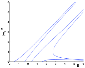
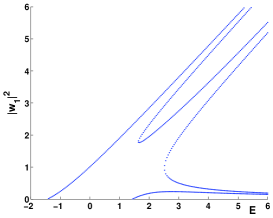
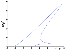
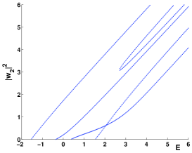
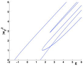
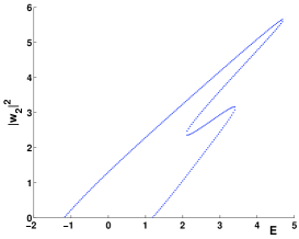
Figure 1: Nonlinear stationary states for $N=2$ and for $\gamma=0.5$ (left), $\gamma=0.75$ (middle), and $\gamma=1.1$ (right). The top and bottom rows show components $|w_{1}|^{2}$ and $|w_{2}|^{2}$ respectively.

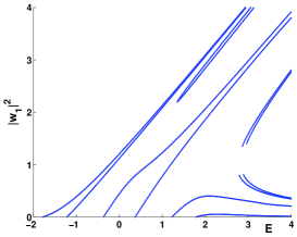
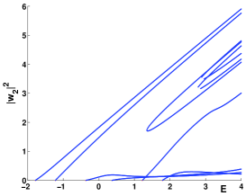
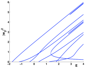
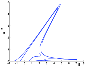
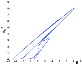
Figure 2: Nonlinear stationary states for $N=3$, and for $\gamma=0.25$ (top) and $\gamma=1.1$ (bottom). The left, middle, and right columns show components $|w_{1}|^{2}$, $|w_{2}|^{2}$, and $|w_{3}|^{2}$ respectively.

For $N=2$, we use the reduction $w_{4}=\bar{w}_{1}$ and $w_{3}=\bar{w}_{2}$. Writing $w_{1}=Ae^{-i\varphi-i\psi}$ and $w_{2}=Be^{-i\psi}$ with real $A$, $B$, $\varphi$, and $\psi$ in the nonlinear stationary dNLS equation (13), we obtain the system of nonlinear equations:

$$\sin(\varphi)=\frac{\gamma A}{B},\quad\sin(2\psi)=\frac{\gamma(A^{2}-B^{2})}{B^{2}}$$ (31)

and

$$A^{3}=AE-B\cos(\varphi),\quad B^{3}=BE-A\cos(\varphi)-B\cos(2\psi).$$ (32)

The roots of the algebraic system (31) and (32) can be investigated numerically and the results depend on the value of $\gamma$. Figure 1 shows the solution branches on the $(E,A^{2})$-plane (top) and the $(E,B^{2})$-plane (bottom) for $\gamma=0.5<\gamma_{2}\approx 0.618$ (left), $\gamma=0.75$ (middle), and $\gamma=1.1$. Note that no solution branches exist for $\gamma>\gamma_{2}^{*}:=2\cos\frac{\pi}{5}\approx 1.618$, because no simple real eigenvalues occur in the linearized dNLS equation (7) for these values of $\gamma$.

According to Theorem 14, we count exactly four ($2N=4$) solution branches for small amplitudes $A$ and $B$ for $\gamma<\gamma_{2}$ and exactly two small solution branches for $\gamma_{2}<\gamma<\gamma_{2}^{*}$. According to Theorem 3, we count exactly four ($2^{N=2}=4$) solution branches for large amplitudes $A$ and $B$ if $\gamma<1$, whereas all solution branches terminate before reaching large amplitudes if $\gamma>1$.

The two branches for small values of $A$ and large values of $E$ are attributed to the solutions in Remark 6. The corresponding values of $B$ are large. On the other hand, no branches exist for large $A$ and small $B$ as $E$ gets large, see Remark 7.

For $N=3$, we write $w_{1}=Ae^{-i(\varphi+\psi+\theta)}=\bar{w}_{6}$, $w_{2}=Be^{-i(\psi+\theta)}=\bar{w}_{5}$, and $w_{3}=Ce^{-i\theta}=\bar{w}_{4}$. The roots of the resulting algebraic system are investigated numerically by a homotopy method and the results are shown on Figure 2. We count six ($2N=6$) branches in the small-amplitude limit if $\gamma<\gamma_{3}\approx 0.445$ and four branches if $\gamma_{3}<\gamma<\gamma^{*}_{3};=2\cos\frac{2\pi}{7}\approx 1.247$. We also count eight ($2^{N=3}=8$) branches for large amplitudes $A^{2}$ if $\gamma<1$ and no branches for large amplitudes $A^{2}$ if $\gamma>1$. More branches are counted for large amplitudes $B^{2}$ and even more branches for large amplitudes $C^{2}$. Overall, the results for $N=3$ are similar to the results for $N=2$.

4 PT-symmetric defects embedded in infinite PT-dNLS lattices

We shall now consider an infinite PT-dNLS lattice, where the particular emphasis is on the existence and stability of localized stationary states (discrete solitons). Because the phase transition in the PT-dNLS equation (1) on the infinite lattice occurs already at $\gamma_{N\to\infty}=0$, there is no way to obtain stable discrete solitons in such systems with extended gain and loss [26]. Therefore, we modify the PT-dNLS lattice by considering the PT-symmetric potential as a finite-size defect. Such defects were considered recently in the physical literature [31] and [4, 5].

Let $N$ be a positive integer and $S_{N}:=\{1,2,...,2N\}$ be the sites of the lattice, where the PT-symmetric defects are placed. The model takes the form

$$i\frac{du_{n}}{dt}=u_{n+1}-2u_{n}+u_{n-1}+i\gamma(-1)^{n}\chi_{n\in S_{N}}u_{n}+|u_{n}|^{2}u_{n},\quad n\in\mathbb{Z},$$ (33)

where $\chi_{n\in S_{N}}$ is a characteristic function for the set $S_{N}$. When $N=1$, the PT-dNLS equation (33) corresponds to the embedded dimer in the infinite PT-dNLS lattice. When $N=2$, it corresponds to the embedded quadrimer, and so on.

We study the linearized PT-dNLS equation and find the phase transition threshold $\tilde{\gamma}_{N}$. It is quite remarkable that $\tilde{\gamma}_{N}>\gamma_{N}$ for any $N\in\mathbb{N}$, in particular, $\tilde{\gamma}_{1}=\sqrt{2}$. Nevertheless, $\tilde{\gamma}_{N}$ is still a monotonically decreasing sequence of $N$ such that $\tilde{\gamma}_{N}\to 0$ as $N\to\infty$.

Then, we employ the large-amplitude (anti-continuum) limit of the PT-dNLS equation (33) to study the existence of discrete solitons supported at the PT-symmetric defect $S_{N}$. For recent results on existence of discrete solitons in the anti-continuum limit for the regular dNLS equation (in the absence of PT-symmetry), see e.g. [3, 11]. We find that for all $\gamma\in(-1,1)$, $2^{N}$ branches of the discrete solitons exist in this limit, for which $|u_{n}|^{2}$ is large for all $n\in S_{N}$.

The existence and stability of discrete solitons is illustrated numerically and we show that the stable branches of the discrete solitons for $\gamma\neq 0$ originate from the stable branches in the Hamiltonian version ($\gamma=0$) of the dNLS equation [25, 27].

4.1 Eigenvalues of the linear PT-dNLS equation

We consider the linear stationary PT-dNLS equation:

$$Ew_{n}=w_{n+1}+w_{n-1}+i\gamma(-1)^{n}\chi_{n\in S_{N}}w_{n},\quad n\in\mathbb{Z}.$$ (34)

Because the PT-symmetric potential is compact, the continuous spectrum of the linear PT-dNLS equation (34) is located for $E\in[-2,2]$. Besides the continuous spectrum, isolated eigenvalues may exist outside the continuous spectrum. To characterize isolated eigenvalues, we introduce a parametrization

$$E:=2\cos\theta,\quad{\rm Re}(\theta)\in[-\pi,\pi],\quad{\rm Im}(\theta)>0,$$ (35)

and look for exponentially decaying solutions of the linear PT-dNLS equation (34) in the form:

$$w_{n}=\left\{\begin{array}[]{lc}w_{1}e^{-i\theta(n-1)},&n\leq 1,\\ w_{2N}e^{i\theta(n-2N)},&\;\;n\geq 2N,\end{array}\right.$$ (36)

which still leaves a set of $2N$ unknown variables $\{w_{n}\}_{n\in S_{N}}$. To find $\{w_{n}\}_{n\in S_{N}}$, we close the linear eigenvalue problem at the algebraic system

$$2\cos\theta w_{n}=w_{n+1}+w_{n-1}+i\gamma(-1)^{n}w_{n},\quad n\in S_{N},$$ (37)

subject to the boundary conditions

$$w_{0}=w_{1}e^{i\theta},\quad w_{2N+1}=w_{2N}e^{i\theta}.$$

Note that each eigenvalue $E$ is complex if ${\rm Im}(\theta)>0$ and there exists a complex conjugate eigenvalue $\bar{E}$ by the PT-symmetry (see also Remark 12). The following result is similar to the result of Theorem 9.

Theorem 4.

A new symmetric pair of complex-conjugate eigenvalues of the linear PT-dNLS equation (34) bifurcates at $|\gamma|=\gamma_{N,k}$, where

$$\gamma_{N,k}:=2\cos\frac{\pi(2k-1)}{4N},\quad 1\leq k\leq N,$$ (38)

and persists for $|\gamma|>\gamma_{N,k}$ except possibly finitely many points on any compact interval of $\gamma$, where the pair coalesces into a double (semi-simple) pair of real eigenvalues. In particular, no complex eigenvalues exist for $\gamma\in(-\tilde{\gamma}_{N},\tilde{\gamma}_{N})$, where

$$\tilde{\gamma}_{N}:=\gamma_{N,k}=2\cos\frac{\pi(2N-1)}{4N}.$$ (39)

Proof.

We set

$$x_{k}=w_{2k-1},\quad y_{k}=w_{2k},\quad 1\leq k\leq N$$

and rewrite the linear eigenvalue problem (37) in the equivalent form:

$$\left\{\begin{array}[]{l}2\cos\theta x_{k}=y_{k-1}+y_{k}-i\gamma x_{k},\\ 2\cos\theta y_{k}=x_{k}+x_{k+1}+i\gamma y_{k},\end{array}\right.\quad 1\leq k\leq N,$$ (40)

subject to the modified boundary conditions $y_{0}=x_{1}e^{i\theta}$ and $x_{N+1}=y_{N}e^{i\theta}$. Expressing $y_{k}$ from the second equation of the system (40) by

$$y_{k}=\frac{x_{k}+x_{k+1}}{2\cos\theta-i\gamma},\quad 1\leq k\leq N-1,\quad y_{N}=\frac{x_{N}}{e^{-i\theta}-i\gamma},$$

and substituting these expressions to the first equation of the system, we obtain a second-order difference equation

$$(\gamma^{2}+4\cos^{2}\theta)x_{k}=x_{k-1}+2x_{k}+x_{k+1},\quad 1\leq k\leq N,$$ (41)

where the boundary conditions are now

$$x_{0}=(e^{i\theta}-i\gamma)e^{i\theta}x_{1},\quad x_{N+1}=\frac{e^{i\theta}x_{N}}{e^{-i\theta}-i\gamma}.$$ (42)

Note that equations (41) are obtained by multiplying every term by $2\cos\theta-i\gamma$, which is hence supposed to be non-zero.

The second-order difference equation (41) admits an exact solution

$$x_{k}=C_{+}e^{i\alpha(k-1)}+C_{-}e^{-i\alpha(k-1)},$$ (43)

where $\alpha$ is defined from the transcendental equation

$$\gamma^{2}+4\cos^{2}\theta=2+2\cos\alpha,$$ (44)

and $(C_{+},C_{-})$ are non-zero solutions of the linear system following from the boundary conditions (42):

$$e^{-i\alpha}C_{+}+e^{i\alpha}C_{-} = (e^{i\theta}-i\gamma)e^{i\theta}(C_{+}+C_{-}),$$

$$(e^{-i\theta}-i\gamma)(C_{+}e^{i\alpha N}+C_{-}e^{-i\alpha N}) = e^{i\theta}(C_{+}e^{i\alpha(N-1)}+C_{-}e^{-i\alpha(N-1)}).$$

Note that for fixed $\gamma$, the values of $\theta$ are obtained from the characteristic equation for this linear homogeneous system, after the values of $\alpha$ are excluded from the transcendental equation (44). Also note that only the values of $\theta$ with ${\rm Im}(\theta)>0$ determine isolated eigenvalues of the linear stationary PT-dNLS equation (34) by means of the representation (35).

After some algebraic manipulations, the characteristic equation for the linear system takes the form

$$\left(\cos(\alpha N)\sin\theta\sin\alpha-i\sin(\alpha N)\cos\theta(1-\cos\alpha)\right)(\gamma+2i\cos\theta)=0.$$

The equation $\gamma+2i\cos\theta=0$ gives an artificial root corresponding to the value $\alpha=\pi$, because the second-order difference equation (41) is obtained by multiplying every term by $2\cos\theta-i\gamma$. Therefore, we drop this nonzero factor from the characteristic equation and reduce it to the transcendental equation

$$e^{2i\theta}=\frac{\sin(N+1)\alpha-\sin N\alpha}{\sin N\alpha-\sin(N-1)\alpha}=\frac{\cos\left(N+\frac{1}{2}\right)\alpha}{\cos\left(N-\frac{1}{2}\right)\alpha}.$$ (45)

Case $N=1$: Equation (45) yields $e^{2i\theta}=2\cos\alpha-1$. When this constraint is used in equation (44), we obtain $e^{-2i\theta}=1-\gamma^{2}$. Since $\gamma\in\mathbb{R}$, we obtain the existence of a simple eigenvalue with ${\rm Re}(\theta)>0$ for $\gamma^{2}>2$ and the bifurcation occurs for $\gamma=\sqrt{2}$ and corresponds to $\theta=\pm\frac{\pi}{2}$, when $\cos\theta=0$.

Case $N\geq 2$: In a general case, we first consider bifurcations of complex values of $\theta$ from real values of $\theta$. Hence, we set $\theta\in\mathbb{R}$ and realize from (44) that ${\rm Im}(\cos\alpha)=0$, which implies either $\alpha\in\mathbb{R}$ or $\alpha\in\pi k+i\mathbb{R}$ for any $k\in\mathbb{Z}$. In both cases, the characteristic equation (45) with real $\theta$ implies that either $\theta=0$ or $\theta=\pm\frac{\pi}{2}$.

If $\theta=0$, then the characteristic equation (45) reduces to the equation $\sin(\alpha N)=0$, whereas equation (44) implies that $\gamma^{2}=-2(1-\cos\alpha)\leq 0$, which is outside of the parameter range we are interested in. (Recall here that no eigenvalues with ${\rm Im}\theta>0$ exist in the self-adjoint case with $\gamma=0$.)

On the other hand, if $\theta=\pm\frac{\pi}{2}$, then the characteristic equation (45) reduces to the equation $\cos(\alpha N)=0$ (recall here that the artificial root $\alpha=\pi$ is neglected) or equivalently,

$$\alpha=\alpha_{k}:=\frac{\pi(2k-1)}{2N},\quad 1\leq k\leq N.$$

From equation (44), we obtain that the bifurcation occurs at

$$\gamma^{2}=\gamma_{k}^{2}:=4\cos^{2}\left(\frac{\alpha_{k}}{2}\right)=4\cos^{2}\left(\frac{\pi(2k-1)}{2N}\right),$$

which corresponds to the values (38).

Next, we show that the values with ${\rm Im}(\theta)>0$ correspond to the range $\gamma^{2}>\gamma_{k}^{2}$. This implies that a new isolated eigenvalue $E$ of the linear stationary PT-dNLS equation (34) with ${\rm Im}(E)\neq 0$ bifurcates from the value $E=0$ that corresponds to $\theta=\pm\frac{\pi}{2}$ at $\gamma=\pm\gamma_{k}$ and persists for all $|\gamma|>\gamma_{k}$. A symmetric complex-conjugate eigenvalue $\bar{E}$ exists by the PT symmetry of the stationary PT-dNLS equation (34).

To show the above claim, we use the parametrization $z:=e^{i\alpha}$, $\zeta:=e^{2i\theta}$, and $s:=\gamma^{2}$. The system of transcendental equations (44) and (45) becomes the system of algebraic equations:

$$z+\frac{1}{z}-\zeta-\frac{1}{\zeta} = s,$$

$$\zeta z(1+z^{2N-1})-z^{2N+1} = 1.$$

We know that for $s=s_{0}:=\gamma_{k}^{2}$, there exists a solution of this algebraic system for $\zeta=-1$ and $z^{2N}=-1$. Therefore, we consider the continuation of this complex-valued root in real values of $s$. By computing the derivative in $s$, we obtain

$$\left[\begin{array}[]{cc}\zeta^{-2}-1&1-z^{-2}\\ z(1+z^{2N-1})&\zeta(1+2Nz^{2N-1})-(2N+1)z^{2N}\end{array}\right]\left[\begin{array}[]{c}\frac{d\zeta}{ds}\\ \frac{dz}{ds}\end{array}\right]=\left[\begin{array}[]{c}1\\ 0\end{array}\right].$$

For $s=s_{0}$, we obtain from this linear system that

$$\frac{d\zeta}{ds}\biggr{|}_{s=s_{0}}=-\frac{2Nz}{(1-z)^{2}}\biggr{|}_{s=s_{0}}=\frac{N}{2\sin^{2}\left(\frac{\alpha_{k}}{2}\right)}$$

and since $\zeta=e^{2i\theta}$, this proves that $\frac{d}{ds}{\rm Im}(\theta)|_{\theta=\pm\frac{\pi}{2}}>0$. By continuity of roots of the algebraic system above, ${\rm Im}(\theta)$ remains positive for $s>s_{0}$, that is, for $\gamma^{2}>\gamma_{k}^{2}$, near the bifurcation point.

We have shown that roots with ${\rm Im}(\theta)>0$ bifurcate from the points $\theta=\pm\frac{\pi}{2}$ and remain in the upper half-plane for all $\gamma^{2}>\gamma_{k}^{2}$. These roots correspond to complex eigenvalues $E$ if ${\rm Re}(\theta)\neq 0$ (in which case $E>2$) or if ${\rm Re}(\theta)\neq\pm\pi$ (in which case $E<2$). Both situations can not be a priori excluded, however, we have here two facts:

• When ${\rm Re}(\theta)=0$ or ${\rm Re}(\theta)=\pm\pi$, a pair of complex-conjugate eigenvalues $E$ coalesce at the real line into a double (semi-simple) eigenvalue, because of the PT-symmetry with ${\rm Im}(\theta)\neq 0$ generates two linearly independent eigenvectors for the same real eigenvalue.

• Roots $\theta$ are analytic with respect to parameter $\gamma$ by analytic dependence of roots of the algebraic system.

Combining these two facts together, we realize that that the double (semi-simple) eigenvalues $E$ can not split along the real axis (as each real eigenvalue after splitting would then become a double eigenvalue by the PT-symmetry). And they can not persist on the real axis as a double eigenvalues because of analyticity of the parameter continuation of roots $\theta$ with respect to $\gamma$. Therefore, these double real roots split back to the complex domain. In addition, analyticity of the parameter continuations guarantees that there are finitely many points on any compact interval in $\gamma$, where the pairs of complex-conjugate eigenvalues can coalesce at the real axis. The proof of the theorem is complete. ∎

We list some numerical values of the phase transition thresholds:

$$\tilde{\gamma}_{1} = 2\cos\frac{\pi}{4}=\sqrt{2},$$

$$\tilde{\gamma}_{2} = 2\cos\frac{3\pi}{8}\approx 0.765,$$

$$\tilde{\gamma}_{3} = 2\cos\frac{5\pi}{12}\approx 0.518,$$

with $\lim_{N\to\infty}\tilde{\gamma}_{N}=0$. Note that $\tilde{\gamma}_{N}>\gamma_{N}$ for any $N\in\mathbb{N}$.

4.2 Stationary states: bifurcations from the anti-continuum limit

We now consider the stationary states, which satisfy the nonlinear stationary PT-dNLS equation

$$Ew_{n}=w_{n+1}+w_{n-1}+i\gamma(-1)^{n}\chi_{n\in S_{N}}w_{n}+|w_{n}|^{2}w_{n},\quad n\in\mathbb{Z}.$$ (47)

We explore the large-amplitude limit similarly to Section 3.3. Hence, we set $E=\frac{1}{\delta}$ and ${\bf w}=\frac{\bf W}{\sqrt{\delta}}$, where $\delta$ is a small positive number. The stationary PT-dNLS equation (47) is rewritten in the equivalent form:

$$(1-|W_{n}|^{2})W_{n}=\delta\left(W_{n+1}+W_{n-1}+i\gamma(-1)^{n}\chi_{n\in S_{N}}W_{n}\right),\quad n\in\mathbb{Z}.$$ (48)

We consider the PT-symmetric solutions with ${\bf W}=P\bar{\bf W}$, where $P$ is given by $[P{\bf W}]_{n}=W_{2N+1-n}$. Note that the choice of $n_{0}$ in $P$ given by Corollary 1 is adjusted to the center of the PT-symmetric defect. Therefore, the existence of the PT-symmetric solutions can be considered in the framework of the following two subsystems:

$$(1-|W_{n}|^{2})W_{n}=\delta\left(W_{n+1}+W_{n-1}+i\gamma(-1)^{n}W_{n}\right),\quad 1\leq n\leq N,$$ (49)

and

$$(1-|W_{n}|^{2})W_{n}=\delta(W_{n+1}+W_{n-1}),\quad n\leq 0,$$ (50)

subject to the boundary condition $W_{N+1}=\bar{W}_{N}$. The following result is similar to the result of Theorem 3.

Theorem 5.

For any $\gamma\in(-1,1)$, the nonlinear stationary PT-dNLS equation (48) in the limit of small positive $\delta$ admits $2^{N}$ PT-symmetric solutions ${\bf W}=P\bar{\bf W}\in l^{2}(\mathbb{Z})$ (unique up to a gauge transformation) such that, for sufficiently small $\delta$, the map $\delta\to{\bf W}$ is $C^{\infty}$ at each solution and there is a positive $\delta$-independent constant $C$ such that

$$\left|{\bf W}-{\bf W}_{0}\right|\leq C\delta,$$ (51)

where ${\bf W}_{0}$ is a solution of Theorem 3 (after rescaling).

Proof.

We consider small solutions of the subsystem (50) for a given $W_{1}\in\mathbb{C}$ and small $\delta\in\mathbb{R}$. Parameter $\gamma\in\mathbb{R}$ is fixed. The nonlinear system represents a bounded $C^{\infty}$ map from $({\bf W}_{-},W_{1},\delta)\in l^{2}(\mathbb{Z}_{-})\times\mathbb{C}\times\mathbb{R}$ to $l^{2}(\mathbb{Z}_{-})$, where $\mathbb{Z}_{-}$ is the set of negative integers including zero. For $\delta=0$ and arbitrary $W_{1}\in\mathbb{C}$, ${\bf W}_{-}={\bf 0}$ is a root of the nonlinear map and the Jacobian with respect to ${\bf W}_{-}$ at ${\bf W}_{-}={\bf 0}$ is invertible. By the Implicit Function Theorem, for all $W_{1}\in\mathbb{C}$ and small $\delta\in\mathbb{R}$, there is a unique solution of the nonlinear system (50) such that the map $(W_{1},\delta)\to{\bf W}_{-}$ is $C^{\infty}$ and there is a positive $\delta$-independent constant $C$ such that $\|{\bf W}_{-}\|_{l^{2}(\mathbb{Z}_{-})}\leq C|\delta|$.

Substituting $W_{0}$ from the map constructed above to the first equation of the subsystem (49), we close the system at $N$ nonlinear equations for $\{W_{n}\}_{1\leq n\leq N}$. The only difference from the $N$ nonlinear equations considered in the proof of Theorem 3 is the boundary condition for given $W_{0}$, however, $W_{0}$ is small as $W_{0}=\mathcal{O}(\delta)$. The two applications of the Implicit Function Theorem developed in the proof of Theorem 3 apply directly to our case and yield the assertion of this theorem. The bound (51) follows from bounds (26) and (28). ∎

Remark 8.

A remark similar to Remark 6 applies on the infinite lattice as well. Besides localized states of Theorem 5, for any $N\geq 2$ and $1\leq M\leq N$, there exist additional soliton states such that $|W_{n}|^{2}\approx 1$ as $\delta\to 0$ for $N-M+1\leq n\leq N+M$ and $|W_{n}|^{2}\approx 0$ as $\delta\to 0$ for $n\leq N-M$ and $n\geq N+M+1$. These stationary states are supported at $2M$ sites near the central sites in the set $S_{N}$.

We give details of the perturbative expansions for the two (most fundamental) discrete solitons supported by the dimer defect for $N=1$. The subsystems (49) and (50) are rewritten explicitly as follows:

$$(1-|W_{1}|^{2})W_{1} = \delta\left(W_{0}+\bar{W}_{1}-i\gamma W_{1}\right),$$ (52)

$$(1-|W_{n}|^{2})W_{n} = \delta\left(W_{n+1}+W_{n-1}\right),\quad\quad n\leq 0.$$ (53)

The perturbation expansion

$$W_{n}=W_{n}^{(0)}+\delta W_{n}^{(1)}+\mathcal{O}(\delta^{2})$$ (54)

allows us to compute at the leading order $W_{n}^{(0)}=e^{-i\theta}\delta_{n,1}$, where $\theta\in[0,\pi]$ is arbitrary at this point. At the $\mathcal{O}(\delta)$ order, we obtain the equations:

$$W_{n}^{(1)} = W_{n+1}^{(0)}+W_{n-1}^{(0)},\quad\quad n\leq 0$$ (55)

$$-\left(e^{-2i\theta}\bar{W}_{1}^{(1)}+W_{1}^{(1)}\right) = e^{i\theta}-i\gamma e^{-i\theta},\quad\quad n=1$$ (56)

Set $W_{1}^{(1)}:=Ze^{-i\theta}$ and rewrite (56) as $-(\bar{Z}+Z)=e^{2i\theta}-i\gamma$. The solvability condition is $\sin(2\theta)=\gamma$ and it gives exactly two values for $\theta\in[0,\pi]$ for any $\gamma\in(-1,1)$. Then, the first-order correction term is found explicitly as follows:

$$W_{n}^{(1)}=-\frac{1}{2}e^{-i\theta}\cos(2\theta)\delta_{n,1}+e^{-i\theta}\delta_{n,2}.$$

The perturbation expansion (54) can be continued to higher orders of $\delta$ thanks to $C^{\infty}$ smoothness in Theorem 5. Hence, we obtain two branches of soliton states supported by the dimer defect.

Remark 9.

The phase transition threshold for $S_{1}$ is $\tilde{\gamma}_{1}=\sqrt{2}$, whereas the soliton states of Theorem 5 are only constructed for $\gamma\in(-1,1)$ in the limit $E\to\infty$. Numerical studies (see Figure 5) show that the solution states exist for $\gamma\in(-1,1)$ for any fixed value of $E$.

4.3 Numerical results

We now test these analytical results for the PT-symmetric chain with embedded defects.

First, we consider the linear limit of such chains and examine the corresponding PT-symmetry phase transitions expected to occur at $\tilde{\gamma}_{N}$. In particular, in Fig. 3, we consider the case of $N=1$, i.e., a single embedded dimer which has been predicted to have a PT-phase transition at $\tilde{\gamma}_{1}=\sqrt{2}$, for the infinite lattice. In the figure, we can clearly discern the relevant transition (the corresponding vertical dashed line shows the theoretical prediction of $\tilde{\gamma}_{1}$). Nevertheless, for the finite lattice considered (here $800$ sites are used), an additional bifurcation is observed at $\gamma=1$ (see also the works of [5, 26]). This bifurcation is suppressed at the infinite lattice limit, but for a finite chain a “bubble” of complex eigenvalues arises around $E=0$ (which is the middle point of the spectral band). This bubble keeps expanding and slowly increasing in imaginary part between $\gamma=1$ and $\gamma=\sqrt{2}$ (notice that this growth is barely visible in the linear scale of the figure but it is noticeable in the logarithmic scale of the inset). At the latter critical point, the rapid growth of the isolated unstable eigenvalue pair becomes dominant for the instability of the lattice with an embedded dimer.

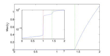
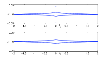
Figure 3: The left panel shows the dependence of the maximal imaginary part $\lambda_{i}$ of the eigenvalues $\lambda=\lambda_{r}+i\lambda_{i}$ versus $\gamma$ for $N=1$. While this is shown in a linear scale with the green dashed line denoting the bifurcation point $\tilde{\gamma}_{1}=\sqrt{2}$, the inset in a semi-logarithmic scale demonstrates the finite-size instability emerging at $\gamma=1$, which is denoted by the red dashed line. The right panel shows the spectrum of the linear PT-dNLS equation (34) for $\gamma=1.43$ (top) and $\gamma=1.4$ (bottom).

Similar conclusions can be drawn for the case of embedded quadrimer ($N=2$) and hexamer ($N=3$) from Fig. 4. The figures reveal, however, that in this case in addition to the actual (infinite chain) critical points of $\tilde{\gamma}_{2}\approx 0.765$ and $\tilde{\gamma}_{3}\approx 0.518$, respectively, there are multiple additional points of weak instability emergence due to finite size effects. Such features are noticeable due to bifurcations of instability bubbles at the edges of the spectral band (at $E=2$ and $E=-2$), at $\gamma\approx 0.46$ for $N=2$ and at $\gamma\approx 0.30$ for $N=3$. Additional bubbles emerge near the middle point of the spectral band (at $E=0$), at $\gamma\approx 0.61$ for $N=2$ and at $\gamma\approx 0.45$ for $N=3$.

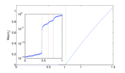
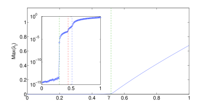
Figure 4: The case of $N=2$ (left panel) and $N=3$ (right panel) for a finite lattice of $800$ sites. The panels are similar to the left panel of Fig. 3, but feature two weak instabilities due to finite size effects (green and red dashed line), in addition to the strong instability at $\tilde{\gamma}_{N}$ (blue dashed line).

Next, we turn to the existence of nonlinear stationary solutions in the PT-symmetric dimer ($N=1$) embedded in the nonlinear chain, as shown in Fig. 5. We have identified two branches of localized states starting from the Hamiltonian limit where $2\theta=0$ and $2\theta=\pi$ (i.e., in-phase and anti-phase discrete solitons, respectively). Indeed, the left panel shows the phase difference between $w_{1}$ and $w_{2}$ for the PT-symmetric embedded dimer. These results clearly illustrate that at the Hamiltonian limit of $\gamma=0$, the system starts from the two well-known in phase and out-of-phase solutions [25]. The former (lower norm one) is unstable for our focusing nonlinearity, while the latter one is spectrally stable. Interestingly, in accordance with what is known for an isolated dimer [20, 28, 31], these two solutions disappear in a saddle-center bifurcation at $\gamma=1$. In fact, both this increased proximity and the eventual collision and disappearance are captured very accurately by the solvability condition $\sin(2\theta)=\gamma$. The resulting angle from the numerical computation and from the essentially coincident analytical prediction are shown in the left panel of Fig. 5. Note that while the results are shown in Fig. 5 for $\delta=0.01$, they remain similar not only for smaller values of $\delta$ (such as e.g. $0.001$), but even for larger values up to $\delta=1$ that were considered. In particular, the point of the saddle-center bifurcation $\gamma=1$ has been found to be identical for other values of $\delta$. This confirms the observation made in Remark 9.

In the Hamiltonian case of $\gamma=0$, our linear stability results for these branches fall back on the analysis of [25]. In fact, we retrieve the exact same condition, for the leading order eigenvalue correction, namely $\lambda^{2}/\delta=4\cos(2\theta)$. This expression reveals the instability of the in-phase mode and the stability (for our focusing nonlinearity) of the out-of-phase one. In the presence of gain/loss (i.e., for finite $\gamma$), the fundamental difference lies in the existence condition which mandates that $\sin(2\theta)=\gamma$ and therefore the eigenvalues of the in-phase unstable state approach the origin (from the real axis), as do the ones of the out-of-phase marginally stable state (from the side of the imaginary axis) as $\gamma$ is increased towards $1$. These eigenvalue pairs end up colliding at the origin at the point of the PT-phase transition at $\gamma=1$. The trajectories of the two sets of eigenvalues are shown in the right panel of Fig. 5. It can be seen that similarly to the Hamiltonian case of [25], the agreement is better for the unstable branch of real eigenvalues. Nevertheless, for both branches the comparison of computation and analysis is highly favorable.

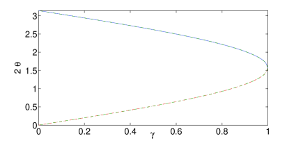
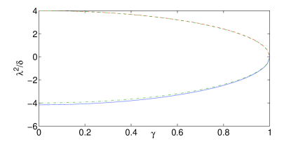
Figure 5: The left panel shows the relative phase $2\theta$ between the two central sites obtained by the numerical computation and the solvability condition $\sin(2\theta)=\gamma$ (a green dash-dotted line). The right panel shows the squared eigenvalue of the linearized PT-dNLS equation at the discrete soliton versus $\gamma$ for each of the two branches. The stable (blue solid) branch of the anti-phase solution (at $\gamma=0$) has a negative $\lambda^{2}$, while the unstable (red dashed) branch of the in-phase solution (at $\gamma=0$) has a positive $\lambda^{2}$. The corresponding theoretical predictions are shown by green dash-dotted lines in very good agreement with the numerical results.

For the case of $N=1$, we now turn to numerical simulations, in order to briefly discuss the difference between the manifestation of the instability of the in-phase localized states for different values of $\gamma$. Two prototypical examples are shown in Fig. 6. Both panels illustrate the evolution of the two most central, maximum amplitude sites of the solution. In the Hamiltonian case of $\gamma=0$ shown in the left panel, it can be seen that small perturbations give rise to an amplified symmetry breaking in the dynamics. Nevertheless, the conservative nature of the ensuing dynamics ascertains the rapid saturation of this symmetry breaking and the eventual oscillations that arise lead to a (nearly) periodic alternation between a symmetric and a symmetry broken state. On the other hand, for $\gamma=0.5$ we observe a drastically different manifestation of this instability shown in the right panel. More specifically, the site associated with gain grows indefinitely in a nearly exponential form, as illustrated in the inset. At the same time, the site associated with damping decreases in amplitude in a similar fashion.

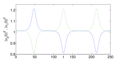
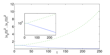
Figure 6: The left panel shows the evolution of the unstable in-phase solution for $\gamma=0$. The amplitude of the central-most two nodes is shown as a function of time. The symmetry-breaking results from the amplification of a noise in the initial data and manifests the instability via a (nearly) periodic recurrence between symmetry-restored and symmetry-broken phases. The right panel shows the same instability for $\gamma=0.5$. The instability leads to an amplification of the gained site amplitude and a decay of the damped site amplitude.

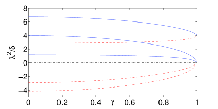
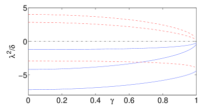
Figure 7: Stability analysis results for the case of $N=2$. The left panel depicts the $++++$ solution (which has three real eigenvalue pairs) by solid (blue) lines, as well as the $+--+$ solution (which has two imaginary and one real pair) by dashed (red) lines. The right panel depicts the $+-+-$ solution (which has three imaginary eigenvalue pairs) by solid (blue) lines, as well as the $++--$ solution (which has two real pairs and one imaginary) by dashed (red) lines. Each pair of these configurations collides and disappears at $\gamma=1$.

Lastly, we address the bifurcation and stability results for the case of $N=2$ i.e., for an embedded quadrimer. In this case, the eigenvalues of the linearization problem are shown in Fig. 7. We have examined four principal configurations with all four sites excited (there exist also configurations with two sites excited as for $N=1$, in accordance with Remark 8). In agreement with Theorem 3, these four configurations are coded as $++++$ (when all sites excited in phase), $+-+-$ (when all sites are out of phase with their immediate neighbors), $++--$, and $+--+$. As can be seen in the figure and as is known from the Hamiltonian limit of $\gamma=0$, the only spectrally stable among these configurations is the out of phase configuration $+-+-$ with three imaginary eigenvalue pairs, while the in-phase configuration $++++$ is the most unstable with three real pairs. Upon continuation over $\gamma$, for both of these configurations, two of the eigenvalue pairs move towards zero (which they reach as $\gamma\rightarrow 1$), while one remains real for the in-phase, and imaginary for the out of phase. Remarkably, pairwise these configurations collide and disappear in the limit of $\gamma\rightarrow 1$. More specifically, the in-phase configuration $++++$ collides with the configuration $+--+$. Similarly the out-of-phase configuration $+-+-$ collides with the configuration $++--$. It should also be noted that we weren’t able to continue any asymmetric mixed phase configurations (such as e.g. $+++-$, $+---$, $-+--$, $--+-$ or their opposite parity variants) past the Hamiltonian limit of $\gamma=0$.

5 Conclusion

In this paper, we examined two distinct scenaria for PT-symmetric dynamical lattices. In the first one, $N$-site PT-symmetric chains were considered as a finite-dimensional dynamical system. In the second one, we have considered the embedding of the finite PT-symmetric system as a defect in an infinite dNLS lattice. In both cases, we have examined the linear problem, explicitly computing the corresponding eigenvalues and identifying the strengths of $\gamma$ beyond which instabilities (and the phase transition breaking the PT-symmetry) arise due to real eigenvalues. We have also considered the nonlinear states when they emerge from the linear limit, as well as when they arise from a highly nonlinear limit under suitable rescaling (analogous to the anti-continuum limit of the standard dNLS lattice). In that case, we argued about the disparity of the branch counts in these two limits (for general $N$), which suggests the existence of a number of bifurcations, such as saddle-center ones, at intermediate values of the corresponding parameter.

In the case of the infinite PT-symmetric PT-dNLS equation,

$$i\frac{du_{n}}{dt}=u_{n+1}-2u_{n}+u_{n-1}+i\gamma(-1)^{n}u_{n}+|u_{n}|^{2}u_{n},\quad n\in\mathbb{Z},$$ (57)

we note that the phase transition threshold is now set at $\gamma_{N\to\infty}=0$. Therefore, for any $\gamma\neq 0$, the linear PT-dNLS equation is unstable with a complex-valued continuous spectrum. Nevertheless, we can still obtain existence of stationary localized states (discrete solitons) in the large-amplitude limit for $\gamma\in(-1,1)$ for any of the configurations described in Theorems 3 and 5. Moreover, the discrete soliton can be centered at any site $n_{0}\in\mathbb{Z}$ because of the shift invariance of the PT-dNLS equation (57).

There are other numerous directions in which one can envision generalizations of the present study. In the present work, we considered the case where there is a single parameter $\gamma$, for each of the $N$ pairs of sites with gain and loss. However, it is also relevant to generalize such considerations to the case of many independent parameters for such sites [34]. On the other hand, one can consider generalizations of the present setting that aim towards the case of higher dimensionality. Arguably, the simplest such generalization concerns the setting of two one-dimensional coupled (across each of their sites) chains in the form of a railroad track as in [30] and the consideration of multi-site excitations therein. However, the genuinely higher dimensional problem and the examination of generalizations of plaquette configurations [21], whereby the potential of vortices exists in the Hamiltonian limit is of particular interest in its own right. These themes will await further consideration.

References

- [1] F.Kh. Abdullaev, Y.V. Kartashov, V.V. Konotop, and D.A. Zezyulin, “Solitons in PT-symmetric nonlinear lattices”, Phys. Rev. A 83 (2011), 041805(R) (4 pages).
- [2] N. V. Alexeeva, I. V. Barashenkov, A.A. Sukhorukov, and Yu.S. Kivshar, “Optical solitons in PT-symmetric nonlinear couplers with gain and loss”, Phys. Rev. A 85 (2012), 063837 (13 pages)
- [3] G.L. Alfimov, V.A. Brazhnyi, and V.V. Konotop, “On classification of intrinsic localized modes for the discrete nonlinear Schrödinger equation”, Physica D 194 (2004), 127–150.
- [4] J. D’Ambroise, P. G. Kevrekidis, and S. Lepri, “Asymmetric wave propagation through nonlinear PT-symmetric oligomers”, J. Phys. A Math. Theor. 45 (2012), 444012 (16 pages)
- [5] J. D’Ambroise, P.G. Kevrekidis, and S. Lepri, “Eigenstates of lattices with embedded PT-symmetric or Hamiltonian oligomer defects”, arXiv:1211.5707.
- [6] T. Azizov and C. Trunk, “On domains of PT symmetric operators related to ”, J. Phys. A: Math. Theor. 43 (2010), 175303 (13 pages)
- [7] T. Azizov and C. Trunk, “PT symmetric, Hermitian and P-self-adjoint operators related to potentials in PT quantum mechanics”, J. Math. Phys. 53 (2012), 012109 (18 pages)
- [8] I.V. Barashenkov, S.V. Suchkov, A.A. Sukhorukov, S.V. Dmitriev and Yu.S. Kivshar, “Breathers in PT-symmetric optical couplers”, Phys. Rev. A 86 (2012) 053809 (12 pages)
- [9] O. Bendix, R. Fleischmann, T. Kottos, and B. Shapiro, “Exponentially fragile PT symmetry in lattices with localized eigenmodes”, Phys. Rev. Lett. 103 (2009), 030402 (4 pages).
- [10] C. M. Bender, “Making Sense of Non-Hermitian Hamiltonians”, Rep. Prog. Phys. 70 (2007) 947–1018.
- [11] C. Chong, D.E. Pelinovsky, and G. Schneider, “On the validity of the variational approximation in discrete nonlinear Schrödinger equations”, Physica D 241 (2012), 115–124.
- [12] S.V. Dmitriev, A.A¿ Sukhorukov, and Yu.S. Kivshar, “Binary parity-time-symmetric nonlinear lattices with balanced gain and loss”, Opt. Lett. 35 (2010), 2976–2978.
- [13] R. Driben and B.A. Malomed, “Stability of solitons in parity-time-symmetric couplers”, Opt. Lett. 36 (2011), 4323–4325.
- [14] R. Driben and B.A. Malomed, “Stabilization of solitons in PT models with supersymmetry by periodic management ”, EPL 96 (2011), 51001 (6 pages).
- [15] E. M. Graefe, H. J. Korsch, and A. E. Niederle, Quantum-classical correspondence for a non-Hermitian Bose-Hubbard dimer, Phys. Rev. A 82 (2010) 013629 (16 pages).
- [16] M. Hiller, T. Kottos, and A. Ossipov, “Bifurcations in resonance widths of an open Bose-Hubbard dimer”, Phys. Rev. A 73 (2006) 063625 (4 pages).
- [17] P.G. Kevrekidis, The Discrete Nonlinear Schr¨odinger Equation: Mathematical Analysis, Numerical Computations and Physical Perspectives, Springer-Verlag (Heidelberg, 2009).
- [18] O.N. Kirillov, “PT-symmetry, indefinite damping and dissipation-induced instabilities”, Phys. Lett. A 376 (2012), 1244–1249.
- [19] V.V. Konotop, D.E. Pelinovsky, and D.A. Zezyulin, “Discrete solitons in PT-symmetric lattices”, EPL 100 (2012), 56006 (6 pages).
- [20] K. Li and P.G. Kevrekidis, “PT-symmetric oligomers: analytical solutions, linear stability, and nonlinear dynamics”, Phys. Rev. E 83 (2011), 066608 (7 pages).
- [21] K. Li, P.G. Kevrekidis, B.A. Malomed, and U. Günther, “Nonlinear PT-symmetric plaquette”, J. Phys. A Math. Theor. 45 (2012) 444021 (23 pages)
- [22] A. Mostafazadeh, “Pseudo-Hermitian Representation of Quantum Mechanics,” Int. J. Geom. Methods Mod. Phys. 7 (2010), 1191–1306.
- [23] Z. H. Musslimani, K. G. Makris, R. El-Ganainy, and D. N. Christodoulides, Optical Solitons in PT Periodic Potentials, Phys. Rev. Lett. 100 (2008) 030402 (4 pages).
- [24] S. Nixon, L. Ge, and J. Yang, “Stability analysis for solitons in PT-symmetric optical lattices”, Phys. Rev. A 85 (2012), 023822 (10 pages).
- [25] D.E. Pelinovsky, P.G. Kevrekidis, and D. Frantzeskakis, “Stability of discrete solitons in nonlinear Schrodinger lattices”, Physica D 212 (2005), 1–19.
- [26] D.E. Pelinovsky, P.G. Kevrekidis, and D.J. Frantzeskakis, “PT-symmetric lattices with extended gain/loss are generically unstable”, EPL 101 (2013), 11002 (6 pages).
- [27] D. Pelinovsky and A. Sakovich, “Internal modes of discrete solitons near the anti-continuum limit of the dNLS equation”, Physica D 240 (2011), 265–281.
- [28] H. Ramezani, T. Kottos, R. El-Ganainy, and D.N. Christodoulides, “Unidirectional nonlinear PT-symmetric optical structures”, Phys. Rev. A 82 (2010), 043803 (6 pages).
- [29] C.E. Rüter, K.G. Makris, R. El-Ganainy, D.N. Christodoulides, M.Segev, and D. Kip, “Observation of parity-time symmetry in optics”, Nature Physics 6 (2010) 192–195.
- [30] S.V. Suchkov, B.A. Malomed, S.V. Dmitriev and Yu.S. Kivshar, “Solitons in a chain of parity-time-invariant dimers”, Phys. Rev. E 84 (2011), 046609.
- [31] A.A. Sukhorukov, S.V. Dmitriev, S.V. Suchkov, and Yu.S. Kivshar, “Nonlocality in PT-symmetric waveguide arrays with gain and loss” Opt. Lett. 37 (2012) 2148-2150.
- [32] A.A. Sukhorukov, Z. Xu, and Yu.S. Kivshar, “Nonlinear suppression of time reversals in PT-symmetric optical couplers” Phys. Rev. A 82 (2010), 043818 (5 pages).
- [33] S. Weigert, “Detecting broken PT-symmetry”, J. Phys. A: Math. Gen. 39 (2006), 10239–10246.
- [34] D.A. Zezyulin and V.V. Konotop, “Nonlinear modes in finite-dimensional PT-symmetric systems” Phys. Rev. Lett. 108 (2012), 213906 (5 pages).