Direct meshless local Petrov-Galerkin (DMLPG) method:
A generalized MLS approximation

Abstract

The Meshless Local Petrov–Galerkin (MLPG) method is one of the popular meshless methods that has been used very successfully to solve several types of boundary value problems since the late nineties. In this paper, using a generalized moving least squares (GMLS) approximation, a new direct MLPG technique, called DMLPG, is presented. Following the principle of meshless methods to express everything “entirely in terms of nodes”, the generalized MLS recovers test functionals directly from values at nodes, without any detour via shape functions. This leads to a cheaper and even more accurate scheme. In particular, the complete absence of shape functions allows numerical integrations in the weak forms of the problem to be done over low–degree polynomials instead of complicated shape functions. Hence, the standard MLS shape function subroutines are not called at all. Numerical examples illustrate the superiority of the new technique over the classical MLPG. On the theoretical side, this paper discusses stability and convergence for the new discretizations that replace those of the standard MLPG. However, it does not treat stability, convergence, or error estimation for the MLPG as a whole. This should be taken from the literature on MLPG.

1 Introduction

The Moving Least Squares method (MLS) was introduced as an approximation technique by Lancaster and Salkauskas [7], inspired by the pioneering work of Shepard [13] and McLain [8, 9]. Since the numerical approximations of MLS are based on a cluster of scattered nodes instead of interpolation on elements, many meshless methods for the numerical solution of differential equations were based on the MLS method in recent years. As an important example of such methods, we mention the Meshless Local Petrov-Galerkin (MLPG) method introduced by S.N. Atluri and his colleagues [1, 2, 3]. It is a truly meshless method in weak form which is based on local subdomains, rather than a single global domain. It requires neither domain elements nor background cells in either the approximation or the integration.

In MLPG and other MLS based methods, the stiffness matrix is provided by integrating over MLS shape functions or their derivatives. These shape functions are complicated and have no closed forms. To get accurate results, numerical quadrature with many integration points is required. Thus the MLS subroutines must be called very often, leading to high computational costs. In contrast to this, the stiffness matrix in finite element methods (FEMs) is constructed by integrating over polynomial basis functions which are much cheaper to evaluate. This relaxes the cost of numerical integrations somewhat. For an account of the importance of numerical integration within meshless methods, we refer the reader to [4].

This paper avoids integration over MLS shape functions in MLPG and replaces it by the much cheaper integration over polynomials. It ignores shape functions completely. Altogether, the method is simpler, faster and more accurate than the original MLPG method. We use a generalized form of the MLS which directly approximates boundary conditions and local weak forms, shifting the numerical integration into the MLS itself, rather than into an outside loop over calls to MLS routines. We call this approach Direct Meshless Local Petrov-Galerkin (DMLPG) method. The convergence rate of MLPG and DMLPG seems to be the same, but thanks to the simplified computation, the results of DMLPG often are more precise than the results of MLPG. All of this is confirmed by numerical examples.

2 Meshless methods

Whatever the given problem is, meshless methods construct solutions from a trial space $U$ whose functions are parametrized “entirely in terms of nodes” [5]. We let these nodes form a set $X:=\{x_{1},\ldots,x_{N}\}$. Then the functions $u$ of the linear trial space $U$ are parametrizable by their values on $X$ iff the linear functionals $\delta_{x_{1}},\ldots,\delta_{x_{N}}$ are linearly independent on $U$. This implies that there must be some basis $u_{1},\ldots,u_{N}$ of $U$ such that the $N\times N$ matrix of values $u_{j}(x_{k})$ is invertible, but we are not interested in knowing or constructing this basis. We only assume that the discretized problem is set up with a vector

$${\makebox{\boldmath$u$}}=(u(x_{1}),\ldots,u(x_{N}))^{T}$$

of unknowns in “meshless” style, and all data have to be expressed in terms of these.

Furthermore, we assume the discretized problem to consist of equations

$$\lambda_{k}(u)=\beta_{k},\;1\leq k\leq M,$$ (2.1)

where we have $M\geq N$ linear functionals $\lambda_{1},\ldots,\lambda_{M}$ and $M$ prescribed real values $\beta_{1},\ldots,\beta_{M}$. Section 4 will describe how this is done for standard linear PDE problems, including the variations of the MLPG.

The upshot of all meshless methods now is to provide good estimates $\widehat{\lambda}_{k}$ of all $\lambda_{k}$ using only values at nodes. This means that one has to find real numbers $a_{j}(\lambda_{k})$ with

$$\widehat{\lambda_{k}(u)}=\displaystyle{\sum_{j=1}^{M}a_{j}(\lambda_{k})u(x_{j})\approx\lambda_{k}(u)}\mbox{ for all }k,\;1\leq k\leq M.$$ (2.2)

Putting the $a_{j}(\lambda_{k})$ into an $M\times N$ matrix $\mathcal{A}$, one has to solve the possibly overdetermined linear system

$$\mathcal{A}\,{\makebox{\boldmath$u$}}={\makebox{\boldmath$b$}}$$ (2.3)

with ${\makebox{\boldmath$b$}}=(\beta_{1},\ldots,\beta_{M})^{T}$.

Note that we do not mention shape functions at all. They are not needed to set up a linear system in terms of values at nodes. The goal just is to find good estimates for the target functionals $\lambda_{k}$ in terms of the values at nodes, e.g. via (2.2), to set up the matrix $\mathcal{A}$. Note that in some cases, e.g. when the functionals $\lambda_{k}$ are derivatives at points, this is just a variation of a finite–difference approach.

In a second stage, users might want to evaluate $u$ at other places than in the nodes $x_{j}$. This is a problem of recovery of functions from discrete data values, and completely independent of PDE solving. There are various possibilities to do so, including the standard MLS with its shape functions, but we do not comment on these techniques here.

3 Generalized moving least squares (GMLS) approximation

Before we show how to discretize PDEs in the form (2.1), we focus on how to find good estimates of functional values $\lambda(u)$ in terms of nodal values $u(x_{1}),\ldots,u(x_{N})$. The classical MLS approximates $\lambda(u)=u(x)$ from nodal values, minimizing a certain weighted discrete $l_{2}$ norm. But in view of the previous section, we need more general functionals. Therefore we employ a generalized version of Moving Least Squares, adapted from [10].

Let $u\in C^{m}(\Omega)$ for some $m\geq 0$, and let $\{\mu_{j}(u)\}_{j=1}^{N}$ be a set of continuous linear functionals $\mu_{j}$ from the dual $C^{m}(\Omega)^{*}$ of $C^{m}(\Omega)$. For a fixed given functional $\lambda\in C^{m}(\Omega)^{*}$, our problem is the approximate recovery of the value $\lambda(u)$ from the values $\{\mu_{j}(u)\}_{j=1}^{N}$. This fits into the preceding section for $\lambda=\lambda_{k},\,1\leq k\leq M$ and $\mu_{j}(u)=u(x_{j}),\,1\leq j\leq N$.

The functionals $\lambda$ and $\mu_{j}$, $1\leq j\leq N$, can, for instance, describe point evaluations of $u$, its derivatives up to order $m$, or some local integrals that contain $u$ or its derivatives in their integrands. In particular, we shall use functionals of the form (4.4) arising from local weak forms, or simple point evaluation functionals on the Dirichlet part of the boundary.

The approximation $\widehat{\lambda(u)}$ of $\lambda(u)$ should be a linear function of the data $\mu_{j}(u)$, i.e. it should have the form

$$\widehat{\lambda(u)}=\sum_{j=1}^{N}a_{j}(\lambda)\mu_{j}(u),$$ (3.1)

and the coefficients $a_{j}$ should be linear in $\lambda$. We already saw this in (2.2). As in the classical MLS, we assume the approximation equation (3.1) to be exact for a finite dimensional subspace $\mathcal{P}=\mathrm{span}\{p_{1},p_{2},\ldots,p_{Q}\}\subset C^{m}(\Omega)$, i.e.

$$\sum_{j=1}^{N}a_{j}(\lambda)\mu_{j}(p)=\lambda(p)\mbox{ for all }p\in\mathcal{P}.$$ (3.2)

As in the classical MLS, we employ the standard technique of minimizing

$$\frac{1}{2}\sum_{j=1}^{N}a_{j}^{2}(\lambda)/w_{j}$$ (3.3)

as a function of the coefficients $a_{j}(\lambda)$ subject to the linear constraints (3.2), where we use positive weights $w_{1},\ldots,w_{N}$ which later will be chosen in a specific way to localize the approximation, provided that $\lambda$ is a functional acting locally. Anyway, the weights should depend on the functionals $\lambda$ and $\mu_{j}$. In most cases, the functional $\lambda$ will be localized at some point $x$, and then we shall use the standard MLS weights for evaluation at $x$.

The GMLS approximation $\widehat{\lambda(u)}$ to $\lambda(u)$ can also be obtained as $\widehat{\lambda(u)}=\lambda(p^{*})$, where $p^{*}\in\mathcal{P}$ is minimizing the weighted least-squares error functional

$$\sum_{j=1}^{N}\big{(}\mu_{j}(u)-\mu_{j}(p)\big{)}^{2}w_{j},$$ (3.4)

among all $p\in\mathcal{P}$. This problem is independent of the functional $\lambda$ and can be efficiently applied for several functionals $\lambda$ for fixed functionals $\mu_{j}$. This may simplify certain calculations a lot, provided that several functionals have to be estimated based on the same local data. Details are in [10], including error bounds for the recovery and a proof that (3.1) holds for $\widehat{\lambda(u)}=\lambda(p^{*})$ with the optimal solution $p^{*}$ of (3.4) and the optimal solution $a_{j}^{*}(\lambda)$ of (3.3). However, in meshless methods, we need more than the single value $\widehat{\lambda(u)}=\lambda(p^{*})$, since we finally need the solution as a vector $a^{*}(\lambda)\in\mathbb{R}^{N}$ with $N$ values $a_{j}^{*}(\lambda),\,1\leq j\leq N$.

In the special case

$$\lambda(u)=(\delta_{x}D^{\alpha})(u),$$ (3.5)

the derivatives of $u$ of order $|\alpha|$ are recovered. They are called GMLS approximation derivatives in [10]. Some authors call them diffuse derivatives, but they not “diffuse” in any way. They are very good direct recoveries of the derivatives of $u$, but not coincident with the corresponding derivatives of the shape functions of the classical MLS solution. Our GMLS approach does not even have shape functions. Instead, derivatives are estimated directly from nodal values, avoiding the inefficient detour via classical derivatives of shape functions.

Note that the use of polynomials is not mandatory, and the resulting values $a_{j}(\lambda)$ will be independent of the chosen basis of $\mathcal{P}$. However, choosing a good basis of $\mathcal{P}$ will improve stability, and the following discussion shows that $\mathcal{P}$ should have the property that $\lambda(p)$ should be easy to evaluate for $p\in\mathcal{P}$.

Even if a different numerical method is used to minimize (3.3) or (3.4), the optimal solution $a^{*}(\lambda)\in\mathbb{R}^{N}$ can be written as

$${a^{*}(\lambda)=WP^{T}(P\,W\,P^{T})^{-1}\lambda({\makebox{\boldmath$p$}})}$$ (3.6)

where $W$ is the diagonal matrix carrying the weights $w_{j}$ on its diagonal, $P$ is the $N\times Q$ matrix of values $\mu_{j}(p_{k}),\;1\leq j\leq N,\,1\leq k\leq Q$, and $\lambda({\makebox{\boldmath$p$}})\in\mathbb{R}^{Q}$ is the vector with values $\lambda(p_{1}),\ldots,\lambda(p_{Q})$ of $\lambda$ on the basis of $\mathcal{P}$. Thus it suffices to evaluate $\lambda$ on the space $\mathcal{P}$, not on a certain trial space spanned by certain shape functions. This will significantly speed up numerical calculations, if the functional $\lambda$ is complicated, e.g. a numerical integration against a test function. Standard examples are functionals of the form

$$\lambda(u)=\int_{K}w(x)\,Lu(x)dx$$

where $L$ is a linear differential operator preserving polynomials or just the identity, and $w$ is some polynomial test or weight function. Such functionals will arise for PDE problems in weak form in the next section. Then our generalized MLS technique will perform integration only over polynomials, if we use polynomials as the space $\mathcal{P}$. Note that this generalizes to any type of functional: we finally just have to evaluate it on a polynomial. No other calls to MLS routines are necessary, because we do not apply the functional to shape functions.

4 Problems in local weak forms

We now write linear PDE problems in the discretized form (2.1), with special emphasis on the Meshless Local Petrov Galerkin Method.

Although the technique proposed in this paper can be used for a wide class of PDEs, we illustrate our approach for the Poisson problem

$$\begin{array}[]{rcll}\Delta u(x)&=&f(x),&x\in\Omega,\\ u(x)&=&u_{D}(x),&x\in\Gamma_{D},\\ \frac{\partial u}{\partial n}(x)&=&u_{N}(x),&x\in\Gamma_{N}\end{array}$$ (4.1)

where $f$ is a given source function, the bounded domain $\Omega\subset\mathbb{R}^{d}$ is enclosed by the boundary $\Gamma=\Gamma_{D}\cup\Gamma_{N}$, $u_{D}$ and $u_{N}$ are the prescribed Dirichlet and Neumann data, respectively, on the Dirichlet boundary $\Gamma_{D}$ and on the Neumann boundary $\Gamma_{N}$, while $n$ is the outward normal direction.

The simplest way of discretizing the problem in the form (2.1) is direct and global collocation. In addition to the trial nodes $x_{1},\ldots,x_{N}$ for obtaining nodal solution values, we can choose finite point sets

$$Y_{\Omega}\subset\Omega,\;Y_{D}\subset\Gamma_{D},\;Y_{N}\subset\Gamma_{N},\;Y:=Y_{\Omega}\cup Y_{D}\cup Y_{N},\;|Y|=M$$

and discretize the problem by $M$ functionals

$$\begin{array}[]{rcrcll}\lambda_{i}(u)&=&\Delta u(z_{i})&=&f(z_{i}),&z_{i}\in Y_{\Omega}\subset\Omega,\\ \lambda_{j}(u)&=&u(z_{j})&=&u_{D}(z_{j}),&z_{j}\in Y_{D}\subset\Gamma_{D},\\ \lambda_{k}(u)&=&\frac{\partial u}{\partial n}(z_{k})&=&u_{N}(z_{k}),&z_{k}\in Y_{N}\subset\Gamma_{N}\end{array}$$ (4.2)

using some proper indexing scheme. In MLPG categories, this is MLPG2 [1, 2]. All functionals are local, and strong in the sense that they do not involve integration over test functions.

For FEM–style global weak discretization, one can keep the second and third part of (4.2), but the first can be weakened using the Divergence Theorem. With sufficiently smooth test functions $v_{i}$, we get

$$\lambda_{i}(u):=\int_{\Gamma}(\nabla u\cdot n)v_{i}\ d\Gamma-\int_{\Omega}\nabla u\cdot\nabla v_{i}\ d\Omega=\int_{\Omega}fv_{i}\ d\Omega$$

as a replacement of the first functionals in (4.2), leading again to (2.1).

Following the original MLPG method, instead of transforming (4.1) into a global weak form, we construct weak forms over local subdomains $\Omega_{\sigma}^{y}$ which are small regions taken around nodes $y$ in the global domain $\Omega$. The local subdomains could theoretically be of any geometric shape and size. But for simplicity they are often taken to be balls $B(y,\sigma)$ intersected with $\Omega$ and centered at $y$ with radius $\sigma$, or squares in 2D or cubes in 3D centered at $y$ with sidelength $\sigma$, denoted by $S(y,\sigma)\cap\Omega$. The variable $\sigma$ parametrizes the local subdomain’s size, and we denote the boundary within $\Omega$ by $\Gamma_{\sigma}^{y}:=\Omega\cap\partial\Omega_{\sigma}^{y}$. We call a node $y$ internal, if the boundary $\partial\Omega_{\sigma}^{y}$ of the local subdomain $\Omega_{\sigma}^{y}$ does not intersect $\Gamma$.

The derivation of the local weak form starts with the local integral

$$\int_{\Omega_{\sigma}^{y}}\big{(}\Delta u-f\big{)}v\ d\Omega=0,$$ (4.3)

where $v$ is an appropriate test function on $\Omega_{\sigma}^{y}$. Employing the Divergence Theorem, we get an equation

$$\lambda_{y,\sigma,v}(u):=\int_{\Gamma_{\sigma}^{y}\setminus\Gamma_{N}}(\nabla u\cdot n)v\ d\Gamma-\int_{\Omega_{\sigma}^{y}}\nabla u\cdot\nabla v\ d\Omega=\int_{\Omega_{\sigma}^{y}}fv\ d\Omega-\int_{\Gamma_{\sigma}^{y}\cap\Gamma_{N}}u_{N}v\ d\Gamma$$ (4.4)

of the form (2.1). For nodes whose subdomain boundary does not intersect $\Gamma_{N}$, the second term on the right–hand side vanishes.

Note that neither Lagrange multipliers nor penalty parameters are introduced into the local weak form, because the Dirichlet boundary conditions are imposed directly using the second line of (4.2) for suitable collocation points, usually taking a subset of the trial nodes.

Some variations of MLPG differ in their choice of functionals (4.4). If the test function $v$ is chosen to vanish on $\Gamma_{\sigma}^{y}\setminus\Gamma_{N}$, the first integral in (4.4) is zero, and we have MLPG1. If the local test function $v$ is the constant 1, the second integral vanishes, and we have MLPG5.

5 Implementation

In this section, we describe the implementation of GMLS approximations to solve the Poisson problem (4.1) using the weak form equations (4.4).

At first we fix $m$, the maximal degree of polynomial basis functions we use. These form the space $\mathcal{P}:=\mathbb{P}_{m}^{d}$ of $d$–variate real–valued polynomials of degree at most $m$. The dimension of this space is $Q={m+d\choose d}$. If the problem has enough smoothness, $m$ will determine the convergence rate.

Then we choose a set $X=\{x_{1},x_{2},...,x_{N}\}\subset\Omega$ of scattered trial points which fills the domain reasonably well, without letting two points come too close to each other. To make this more precise, we need the quantities fill distance and separation distance which are important to measure the quality of centers and derive rates of convergence. For a set of points $X=\{x_{1},x_{2},...,x_{N}\}$ in a bounded domain $\Omega\subseteq\mathbb{R}^{d}$, the fill distance is defined to be

$$h_{X,\Omega}=\sup_{x\in\Omega}\min_{1\leq j\leq N}\|x-x_{j}\|_{2},$$

and the separation distance is defined by

$$q_{X}=\frac{1}{2}\min_{i\neq j}\|x_{i}-x_{j}\|_{2}.$$

A set $X$ of data sites is said to be quasi-uniform with respect to a constant $c_{\mathrm{qu}}>0$ if

$$q_{X}\leq h_{X,\Omega}\leq c_{\mathrm{qu}}q_{X}.$$ (5.1)

In this sense, we require the set $X$ of trial nodes to be quasi–uniform.

We now have to define the functionals $\lambda_{1},\ldots,\lambda_{M}$ discretizing our PDE problem. This requires a selection between MLPG1, MLPG2, and MLPG5, and the decision to use oversampling or not, i.e. $M>N$ or $M=N$. Oversampling will often increase stability at increased cost, but we found that in our examples it was not necessary. Since we have to execute the GMLS method for each functional $\lambda_{k}$, approximating it in terms of function values at the trial nodes in $B(y_{k},\delta)\cap X$, we have to make sure that the GMLS does not break down. This means that the matrix $\mathcal{B}$ of (3.6) must have rank $Q$, if formed for the nodes in $B(y_{k},\delta)\cap X$. In general:

Definition 5.1.

A set $Z$ of pairwise distinct points in $\mathbb{R}^{d}$ is called $\mathbb{P}_{m}^{d}$-unisolvent if the zero polynomial is the only polynomial from $\mathbb{P}_{m}^{d}$ which vanishes on $Z$.

To give a sufficient condition for unisolvency, we need

Definition 5.2.

A set $\Omega\subset\mathbb{R}^{d}$ is said to satisfy an interior cone condition if there exists an angle $\theta\in(0,\pi/2)$ and a radius $r>0$ such that for every $x\in\Omega$ a unit vector $\xi(x)$ exists such that the cone

$$C(x,\xi,\theta,r):=\big{\{}x+ty:y\in\mathbb{R}^{d},\|y\|_{2}=1,y^{T}\xi\geq\cos\theta,t\in[0,r]\big{\}}$$

is contained in $\Omega$.

Theorem 5.3.

([12], see also [14])
For any compact domain $\Omega$ in $\mathbb{R}^{d}$ with an interior cone condition, and any $m\geq 0$ there are positive constants $h_{0}$ and $c_{0}$ such that for all trial node sets $X$ with fill distance $h_{X,\Omega}\leq h_{0}$, all test points $y\in\Omega$, and all radii $\delta\geq c_{0}\,h_{X,\Omega}$, the set $B(y,\delta)\cap X$ is $\mathbb{P}_{m}^{d}$–unisolvent.

This means that the placement of test nodes and the choice of weight function supports can be linked to the fill distance of the set of trial nodes. Oversampling never causes problems, if the weight function support radius is kept proportional to the fill distance of the trial nodes.

Some test nodes should be scattered over the Dirichlet boundary $\Gamma_{D}$ to impose the Dirichlet boundary conditions. Like in the collocation case, we denote the subset of these points by $Y_{D}\subset Y\cap\Gamma_{D}$. For MLPG2, we similarly define $Y_{N}$, and then the setup of the functionals simply follows (4.2), with or without oversampling. In principle, the sets $Y_{\Omega},\,Y_{N},\,Y_{D}$ need not be disjoint.

For weak problems in MLPG1 or MLPG5 form, we just implement the functionals $\lambda_{y_{k},\sigma_{k},v_{k}}$ of (4.4) as described in Section 4. Altogether, we follow Section 2 by implementing (2.1) via (2.2), and ending with the system (2.3).

The order of convergence of the approximated functional to its exact value is important in this case. Applying the same strategy presented in [10] for $\lambda_{y,\alpha}(u):=D^{\alpha}u(y)$, we can prove

Theorem 5.4.

Let

$$\lambda(u)=\lambda_{y,\sigma,w}(u):=\int_{K}w(x)\,Lu(x)dx,\quad K=\Omega_{\sigma}^{y}\mbox{ or }\partial\Omega_{\sigma}^{y},\,y\in\Omega_{\sigma}^{y}.$$

In the situation of Theorem 5.3, define $\Omega^{*}$ to be the closure of $\bigcup_{x\in\Omega}B(x,\delta)$. Define

$$\widehat{\lambda(u)}:=\sum_{j=1}^{N}a^{*}_{j}(\lambda)u(x_{j}),$$

where $a^{*}_{j}(\lambda)$ are functions derived from the GMLS approximation in (3.6). Then there exists a constant $c>0$ such that for all $u\in C^{m+1}(\Omega^{*})$ and all quasi-uniform $X\subset\Omega$ with $h_{X,\Omega}\leq h_{0}$ we have

$$\left\|\lambda(u)-\widehat{\lambda(u)}\right\|_{L_{\infty}(\Omega)}\leq ch_{X,\Omega}^{m+1-n}|u|_{C^{m+1}(\Omega^{*})},$$ (5.2)

providing $\int_{K}|w(x)|dx<\infty$ and if $\lambda(u)\neq 0$, $\int_{K}w(x)\,Lx^{\alpha}dx\neq 0$ ($\lambda(x^{\alpha})\neq 0$) for some $\alpha$ with $|\alpha|=m$. Here $n$ is the maximal order of derivatives involved in linear operator $L$ and $|u|_{C^{m+1}(\Omega^{*})}:=\max_{|\alpha|=m+1}\|D^{\alpha}u\|_{L_{\infty}(\Omega)}$.

However, we cannot guarantee that the system (2.3) has full rank, since we only made sure that the rows of the system can be calculated via the GMLS if Theorem 5.3 applies. Oversampling will usually help if the system causes problems.

After the solution vector $u$ of (2.3), consisting of values $u(x_{j})$ of values at the trial nodes is determined by solving the system, other values of the solution function $u(x)$ (and also its derivatives) can be calculated in every point $x\in\Omega$ again using the MLS approximation.

Since we have direct approximations for boundary conditions and local weak forms, this method is called direct meshless local Petrov-Galerkin (DMLPG) method. It comes in the DMLPG1, DMLPG2, and DMLPG5 variations.

In contrast to MLPG2, if the GMLS derivatives (“diffuse” derivatives) [10] are used instead of the standard derivatives of MLS shape functions, we have DMLPG2. As investigated in [10], the accuracies for calculating the matrix $\mathcal{A}$ of (2.3) are the same, but the computational cost of DMLPG2 is less. When looking into the literature, we found that DMLPG2 coincides with the Diffuse Approximate Method (DAM) [11]. But since we avoid using the word diffuse because there is nothing “diffuse” about these derivatives [10], we will call the method DMLPG2 or direct MLS collocation (DMLSC) method.

As we saw in Section 3, in DMLPG1/5 methods the integrations are done only over polynomials, if the latter are used in the GMLS. For every functional $\lambda_{k}$, $1\leq k\leq M\geq N$, the GMLS routine is called only once. There are no calls to produce values of shape functions. The standard MLPG/MLS technique at degree $m$ implements numerical integration by calling shape function evaluations, and thus the MLS routine is called approximatively $M\,K$ times where $K$ is the average number of integration points. Moreover, in standard MLPG methods the derivatives of MLS shape function must also be provided, while DMLPG has no shape functions at all. Consequently, DMLPG is considerably faster than MLPG. In addition, due to the error analysis presented in Theorem 5.4 for the new GMLS method, the final accuracies of both MLPG and DMLPG methods are the same. We will see experimentally that DMLPG is even more accurate than MLPG.

As highlighted in [4], numerical integration in FEM is simple because the integrands of the elements of the stiffness matrix are polynomials. In contrast to this, the shape functions used in standard meshless methods are much more costly to evaluate, making numerical integration a much bigger challenge than for the FEM. In MLPG methods, numerical integrations are simpler than for various other meshless methods, since the local weak form breaks everything down to local well–shaped subdomains. However, since the integrands are based on MLS shape functions and their derivatives, a Gauss quadrature with many points is required to get accurate results, especially when the density of nodes increases. Overcoming this drawback is a major advantage of DMLPG methods, because the integrations are done over polynomials, like in FEM.

It is interesting to note that if local sub-domains are chosen in DMLPG5 as $S(x,\sigma)$ (square or cube), a $(d-1)$–times $\left\lceil\frac{m}{2}\right\rceil$–points Gauss quadrature gives the exact solution for local boundary integrals around the nodes in the interior of $\Omega$. In DMLPG1, if again $S(x,\sigma)$ is chosen as a local sub-domain and if a polynomial test function is employed, a $d$-times $\left\lceil\frac{(m-1)(n-1)+1}{2}\right\rceil$–points Gauss quadrature is enough to get exact interior local domain integrals. Here, $n$ is the degree of the polynomial test function. As a polynomial test function on the square or cube for DMLPG1 with $n=2$, we can use

$$v(x;x_{k})=\left\{\begin{split}\prod_{i=1}^{d}\left(1-\frac{4}{\sigma^{2}}(\xi_{i}-\xi_{ki})^{2}\right),&\quad x\in S(x_{k},\sigma),\\ 0,\quad\quad\quad\quad\quad\quad\quad\quad&\quad\mbox{otherwise}\end{split}\right.$$

where $x=(\xi_{1},...,\xi_{d})$ and $x_{k}=(\xi_{k1},...,\xi_{kd})$. In DMLPG1 with balls as sub-domains, weight functions of the form function

$$w_{\delta}(x,y)=\phi\left(\frac{\|x-y\|_{2}}{\delta}\right),$$ (5.3)

with $\delta=\sigma$ can be used as test functions. Both of these test functions vanish on $\Gamma_{\sigma}^{x_{k}}\backslash\Gamma_{N}$, as required in DMLPG1.

Note that, if the second weak forms (Green forms) are taken over local sub-domains and a modified fundamental solution is used as test function, the process gives the DMLPG4 rather than MLPG4 or the meshless LBIE method presented in [15]. In DMLPG4, it is better to use balls as local sub-domains, because in this case the modified fundamental solution, used as a test function, can be derived easily. But the test function is not a polynomial.

The trial and test functions in both MLPG3 and 6 come from the same space and thus they are Galerkin type techniques. If we formulate the analogues DMLPG3/6, the integrands include shape functions again. Therefore, they annihilate the advantages of DMLPG methods with respect to numerical integration, and we ignore them in favour of keeping all benefits of DMLPG methods.

Instead, we add some remarks about selecting $m$, the degree of polynomial basis functions in the GMLS. For $m=1$, the variants DMLPG 1, 4, and 5 will necessarily fail. The background is that the GMLS performs an optimal recovery of a functional $\lambda$ in terms of nodal values, and the recovery is exact on a subspace $\mathcal{P}$, using minimal coefficients at the nodal values. Thus, in all cases where the functional is zero on $\mathcal{P}$ by some reason or other, the recovery formula will be zero and will generate a zero row in the stiffness matrix. This happens for all variations based on functionals (4.4) and functionals extracted from the second weak form on interior points, since all those functionals are reformulations of

$$\lambda_{y,\sigma,v}(u)=\int_{B(y,\sigma)}v\,\Delta u\,d\omega$$

and thus vanish on harmonic functions $u$, in particular on linear functions. Thus, for solving inhomogeneous problems, users should pick spaces $\mathcal{P}$ of non–harmonic functions, if they employ GMLS with exactness on $\mathcal{P}$. This rules out polynomials with degree $m\leq 1$.

Another closely related point arises from symmetry of subdomains. Since polynomials in a ball $B(x,\sigma)$ or a cube $S(x,\sigma)$ have symmetry properties, the entries of stiffness matrices in rows corresponding to internal points will often be the same for $m=2k$ and $m=2k+1$. Thus convergence rates often do not increase when going from $m=2$ to $m=3$, for instance. But this observation affects MLPG and DMLPG in the same way.

6 Stability and convergence

For the classical MLS and the generalized MLS from [10] and Theorem 5.4 it is known that the recovery $\widehat{\lambda(u^{*})}$ of values of functionals $\lambda$ on a true solution $u^{*}$ has an error of order $\mathcal{O}(h^{m+1-k})$, if $h$ is the fill distance of the trial nodes, $m$ is the degree of polynomials used locally, if the exact solution $u^{*}$ is at least $C^{m+1}$, $k$ is the maximal order of derivatives of $u^{*}$ involved in the functional, and if numerical integration has an even smaller error. In particular, the classical MLS and the new GMLS produce roughly the same stiffness matrices, but the GMLS has a considerably smaller computational complexity.

However, the error committed in the approximation of the test functionals in terms of function values at nodes does not always carry over to the convergence rate of the full algorithm, since there is no stability analysis, so far. Even if perfect stability would hold, the best one can expect is to get the convergence rate implied by the local trial approximation, i.e. by local polynomials of degree $m$. This would again mean a rate of $\mathcal{O}(h^{m+1-k})$, but only if the solution is indeed locally approximated by polynomials of that degree. In fact, the next section will show that this rate can often be observed. But our symmetry arguments at the end of the previous section show that sometimes the degree $m=2k+1$ cannot improve the behavior for $m=2k$, because the odd–degree polynomials simply do not show up in most of the calculations for the stiffness matrix.

7 Numerical results

In this section some numerical results are presented to demonstrate the efficiency of DMLPG methods and its advantages over MLPG methods. We consider the Poisson equation (4.1) on the square $[0,1]^{2}\subset\mathbb{R}^{2}$ with Dirichlet boundary conditions. Since we want to study convergence rates without being limited by smnoothness of the solution, we take Franke’s function [6]

$$\begin{split}u(\bar{x},\bar{y})=&\frac{3}{4}e^{-1/4((9\bar{x}-2)^{2}+(9\bar{y}-2)^{2})}+\frac{3}{4}e^{-(1/49)(9\bar{x}+1)^{2}-(1/10)(9\bar{y}+1)^{2})}\\ &~{}+\frac{1}{2}e^{-1/4((9\bar{x}-7)^{2}+(9\bar{y}-3)^{2})}-\frac{1}{5}e^{-(9\bar{x}-4)^{2}-(9\bar{y}-7)^{2}},\end{split}$$

where $(\bar{x},\bar{y})$ denotes the two components of $x\in\mathbb{R}^{2}$, as analytical solution and calculate the right hand side and boundary conditions accordingly. Note that Franke’s function is a standard test function for 2D scattered data fitting. Regular mesh distributions with mesh-size $h$ are provided in all cases, though the methods would work with scattered data. We do not implement oversampling in the results of this paper. In fact, the trial and test points are chosen to be coincident. Also, the shifted scaled polynomial

$$\left\{\frac{(x-z)^{\alpha}}{h^{|\alpha|}}\right\}_{0\leq|\alpha|\leq m},$$

where $z$ is a fixed evaluation point such as a test point or a Gaussian point for integration, is used instead of the natural polynomial basis $\{x^{\alpha}\}_{0\leq|\alpha|\leq m}$ for MLS approximation. In [10], it is shown that this choice of basis function leads to more stable and accurate MLS approximation. We use the shifted scaled basis for both MLPG5 and DMLPG5 methods with $m=2,3$ and $4$. The Gaussian weight function

$$w_{\delta}(x,x_{j})=\left\{\begin{split}\frac{\exp\big{(}-(\|x-x_{j}\|_{2}/c)^{2}\big{)}-\exp\big{(}-(\delta/c)^{2}\big{)}}{1-\exp\big{(}-(\delta/c)^{2}\big{)}},&\quad 0\leq\|x-x_{j}\|_{2}\leq\delta,\\ 0,\quad\quad\quad\quad\quad\quad\quad\quad&\quad\|x-x_{j}\|_{2}>\delta\end{split}\right.$$

is employed where $c=c_{0}h$ is a constant controlling the shape of the weight function and $\delta=\delta_{0}h$ is the size of the support domains.

Let $m=2$ and set $c_{0}=0.6$ and $\delta_{0}=2m$. At first the local sub-domains are taken to be circles. To get the best results in MLPG we have to use an accurate quadrature formula. Here a 20-points regular Gauss-Legendre quadrature is employed for numerical integrations over local sub-domains.

Numerical results, for different mesh-sizes $h$, are presented in terms of maximum errors, ratios and CPU times used for MLPG5 and DMLPG5 in Tables 1.

Table 1. The maximum errors, ratios and CPU times used for MLPG5 and DMLPG5 with $m=2$
			MLPG5				DMLPG5				CPU time used
	$h$		$\|e\|_{\infty}$		ratio		$\|e\|_{\infty}$		ratio		MLPG5		DMLPG5
	$0.2$		$0.44\times 10^{-1}$		$-$		$0.23\times 10^{-1}$		$-$		$0.4$ sec.		$0.2$ sec.
	$0.1$		$0.15\times 10^{-1}$		$1.59$		$0.72\times 10^{-2}$		$1.68$		$1.2$		$0.3$
	$0.05$		$0.73\times 10^{-2}$		$0.99$		$0.20\times 10^{-2}$		$1.84$		$6.5$		$1.4$
	$0.025$		$0.24\times 10^{-2}$		$1.61$		$0.58\times 10^{-3}$		$1.80$		$68.5$		$6.5$
	$0.0125$		$0.66\times 10^{-3}$		$1.85$		$0.14\times 10^{-3}$		$1.98$		$2016.0$		$52.1$

The mesh-size $h$ is divided by two row by row, therefore the ratios are computed by

$$\log_{2}\left(\frac{\|e({h})\|_{\infty}}{\|e({h/2})\|_{\infty}}\right).$$

Both methods have nearly the same order 2, which cannot be improved for this trial space, since the expected optimal order is $m+1-k=3-1=2$. But significant differences occur in the columns with CPU times. As we stated before, this is due to restricting local integrations to polynomial basis functions in DMLPG rather than to integrate over MLS shape functions in the original MLPG. We could get the same results with fewer integration points for DMLPG, but to be fair in comparison, we use the same quadrature.

In addition, to give more insight into the errors, the maximum errors of MLPG5 and DMLPG5 are illustrated in Fig. 1. Once can see that DMLPG is more accurate, maybe due to avoiding many computations and hence many roundoff errors.

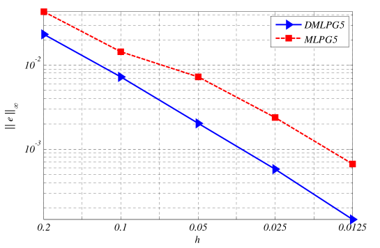
Figure 1: Comparison of MLPG5 and DMLPG5 in terms of maximum errors for $m=2$.

In Table 2 and Fig. 2, we have compared MLPG5 and DMLPG5 in case $m=3$. The convergence rate stays at 2 for both methods, since the third–degree polynomials cannot contribute to the weak form. The figure shows approximately the same error results. But the CPU times used are indeed different.

Table 2. The maximum errors, ratios and CPU times used for MLPG5 and DMLPG5 with $m=3$
			MLPG5				DMLPG5				CPU time used
	$h$		$\|e\|_{\infty}$		ratio		$\|e\|_{\infty}$		ratio		MLPG5		DMLPG5
	$0.2$		$0.28\times 10^{-1}$		$-$		$0.23\times 10^{-1}$		$-$		$0.8$ sec.		$0.2$ sec.
	$0.1$		$0.13\times 10^{-1}$		$1.08$		$0.74\times 10^{-2}$		$1.62$		$1.8$		$0.4$
	$0.05$		$0.33\times 10^{-2}$		$1.98$		$0.20\times 10^{-2}$		$1.89$		$9.7$		$1.6$
	$0.025$		$0.78\times 10^{-3}$		$2.09$		$0.58\times 10^{-3}$		$1.80$		$87.7$		$7.6$
	$0.0125$		$0.19\times 10^{-3}$		$2.06$		$0.15\times 10^{-3}$		$1.98$		$2293.3$		$56.1$

Figure 2: Comparison of MLPG5 and DMLPG5 in terms of maximum errors for $m=3$.

In the results presented up to here, we used balls (circles) as local sub-domains. Now we turn to use squares for both MLPG5 and DMLPG5. Also, we run the programs with $m=4$ to see the differences. The parameters $c_{0}=0.8$ and $\delta_{0}=2m$ are selected. In DMLPG5, a 2-points Gaussian quadrature is enough to get exact numerical integrations. But for MLPG5 and the right hand sides we use a 10-points Gaussian quadrature for every sides of squares. The results are depicted in Table 3 and Fig. 3. DMLPG is more accurate and approximately gives the full order $4$ in this case. Beside, as we expected, the computational cost of DMLPG is remarkably less than MLPG.

Table 3. The maximum errors, ratios and CPU times used for MLPG5 and DMLPG5 with $m=4$
			MLPG5				DMLPG5				CPU time used
	$h$		$\|e\|_{\infty}$		ratio		$\|e\|_{\infty}$		ratio		MLPG5		DMLPG5
	$0.2$		$0.10\times 10^{0}$		$-$		$0.12\times 10^{0}$		$-$		$0.5$ sec.		$0.2$ sec.
	$0.1$		$0.25\times 10^{-1}$		$2.04$		$0.17\times 10^{-1}$		$2.87$		$2.7$		$0.2$
	$0.05$		$0.78\times 10^{-2}$		$1.66$		$0.12\times 10^{-2}$		$3.75$		$19.2$		$0.9$
	$0.025$		$0.79\times 10^{-3}$		$3.30$		$0.75\times 10^{-4}$		$4.04$		$142.2$		$4.7$
	$0.0125$		$0.55\times 10^{-4}$		$3.86$		$0.43\times 10^{-5}$		$4.12$		$2604.9$		$43.9$

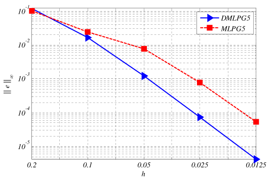
Figure 3: Comparison of MLPG5 and DMLPG5 in terms of maximum errors for $m=4$.

Results for MLPG1 and DMLPG1 turn out to behave similarly. As we know, MLPG1 is more expensive than MLPG5 [1, 2], but there is no significant difference between computational costs of DMLPG5 and DMLPG1. Therefore the differences between CPU times used for MLPG1 and DMLPG1 are absolutely larger.

All routines were written using Matlab^© and run on a Pentium 4 PC with 2.50 GB of Memory and a twin–core 2.00 GHz CPU.

8 Conclusion

This article describes a new MLPG method, called DMLPG method, based on generalized moving least squares (GMLS) approximation for solving boundary value problems. The new method is considerably faster than the classical MLPG variants, because

• direct approximations of data functionals are used for Dirichlet boundary conditions and local weak forms,

• local integrations are done over polynomials rather than over complicated MLS shape functions,

• numerical integrations can sometimes be performed exactly.

The convergence rate of both methods should be the same, but thanks to avoiding many computations and roundoff errors, and of course by treating the numerical integrations in a more elegant and possibly exact way, the results of DMLPG turn often out to be more accurate than the results of MLPG.

On the downside, DMLPG does not work for $m=1$ since it locally uses (harmonic) linear functions instead of complicated shape functions. But most MLPG users choose higher degrees anyway, in order to obtain better convergence rates.

Altogether, we believe that the DMLPG methods have great potential to replace the original MLPG methods in many situations.

References

- [1] S. N. Atluri, The meshless method (MLPG) for domain and BIE discretizations, Tech Science Press, Encino, CA, 2005.
- [2] S. N. Atluri, S. Shen, The Meshless Local Petrov-Galerkin (MLPG) Method, Tech Science Press, Encino, CA, 2002.
- [3] S. N. Atluri, T.-L. Zhu, A new meshless local Petrov-Galerkin (MLPG) approach in Computational Mechanics, Computational Mechanics 22 (1998) 117–127.
- [4] I. Babuska, U. Banerjee, J. Osborn, Q. Zhang, Effect of numerical integration on meshless methods, Comput. Methods Appl. Mech. Engrg. 198 (2009) 27–40.
- [5] T. Belytschko, Y. Krongauz, D. Organ, M. Fleming, P. Krysl, Meshless methods: an overview and recent developments, Computer Methods in Applied Mechanics and Engineering, special issue 139 (1996) 3–47.
- [6] R. Franke, Scattered data interpolation: tests of some methods, Mathematics of Computation 48 (1982) 181–200.
- [7] P. Lancaster, K. Salkauskas, Surfaces generated by moving least squares methods, Mathematics of Computation 37 (1981) 141–158.
- [8] D. McLain, Drawing contours from arbitrary data points, Computer Journal 17 (1974) 318–324.
- [9] D. McLain, Two dimensional interpolation from random data, Comput. J. 19 (1976) 178–181.
- [10] D. Mirzaei, R. Schaback, M. Dehghan, On generalized moving least squares and diffuse derivatives, IMA J. Numer. Anal. 32, No. 3 (2012) 983–1000, doi: 10.1093/imanum/drr030.
- [11] C. Prax, H. Sadat, P. Salagnac, Diffuse approximation method for solving natural convection in porous media, Transport in Porous Media 22 (1996) 215–223.
- [12] R. Schaback, Kernel–based meshless methods, lecture Note, Göttingen (2011).
- [13] D. Shepard, A two-dimensional interpolation function for irregularly-spaced data, in: Proceedings of the 23th National Conference ACM, ACM New York, 1968, pp. 517–523.
- [14] H. Wendland, Scattered Data Approximation, Cambridge University Press, 2005.
- [15] T. Zhu, J. Zhang, S. Atluri, A local boundary integral equation (LBIE) method in computational mechanics, and a meshless discretization approach, Comput. Mech. 21 (1998) 223–235.