The vector coupling $\alpha_{\rm V}(r)$ and the scales $r_{0},~{}r_{1}$ in the background perturbation theory

Abstract

We study the universal static potential $V_{\rm st}(r)$ and the force, which are fully determined by two fundamental parameters: the string tension $\sigma=0.18\pm 0.02$ GeV² and the QCD constants $\Lambda_{\overline{\rm MS}}(n_{f})$, taken from pQCD, while the infrared (IR) regulator $M_{\rm B}$ is taken from the background perturbation theory and expressed via the string tension. The vector couplings $\alpha_{\rm V}(r)$ in the static potential and $\alpha_{\rm F}(r)$ in the static force, as well as the characteristic scales, $r_{1}(n_{f}=3)$ and $r_{0}(n_{f}=3)$, are calculated and compared to lattice data. The result $r_{0}\Lambda_{\overline{\rm MS}}(n_{f}=3)=0.77\pm 0.03$, which agrees with the lattice data, is obtained for $M_{\rm B}=(1.15\pm 0.02)$ GeV. However, better agreement with the bottomonium spectrum is reached for a smaller $\Lambda_{\overline{\rm MS}}(n_{f}=3)=(325\pm 15)$ MeV and the frozen value of $\alpha_{V}=0.57\pm 0.02$. The mass splittings $\bar{M}(1D)-\bar{M}(1P)$ and $\bar{M}(2P)-\bar{M}(1P)$ are shown to be sensitive to the IR regulator used. The masses $M(1\,^{3}D_{3})=10169(2)$ MeV and $M(1\,^{3}D_{1})=10155(3)$ MeV are predicted.

I Introduction

The Hamiltonian formalism may be considered as a powerful tool to study such hadron properties as meson spectroscopy, including high excitations, hyperfine and fine-structure splittings of different meson multiplets, leptonic widths, and radiative and strong meson decays. For decades, different phenomenological Hamiltonians were used in constituent quark models, and some of them were rather successful in predictions of meson properties for low-lying states ref.1 ; ref.2 ; ref.3 ; ref.4 ; ref.5 . However, in such models the quark-antiquark potentials contain a large number of arbitrary parameters like constituent quark masses, variable values of the string tension and the QCD constant $\Lambda$, as well as an overall additive fitting constant. Meanwhile, the relativistic string Hamiltonian (RSH) $H_{\rm R}$, which was derived from the gauge-invariant meson Green’s function with the use of the QCD Lagrangian ref.6 , contains a minimal set of fundamental parameters: the current-quark masses, the string tension $\sigma$ fixed by the slope of the Regge trajectories for light mesons, and the QCD constant $\Lambda(n_{f})$, which can be taken from perturbative QCD (pQCD). It is important that in the RSH the spin-independent static potential $V_{\rm st}(r)$ is universal and applicable for different $q_{1}\bar{q}_{2}$ mesons with arbitrary masses (including $m_{q}=0$). This potential is defined via the vacuum average over the Wilson loop $\langle W(C)\rangle$ ref.6 ; ref.7 ; ref.8 ; ref.9 ; ref.10 ; ref.11 and the only approximation made is that $\langle W(C)\rangle$ is taken in the form of the minimal area law, which appears to be a good approximation for separations $r\mathrel{\mathchoice{\lower 3.6pt\vbox{\halign{$\mathsurround=0pt\displaystyle\hfil#\hfil$\cr>\crcr\sim\crcr}}}{\lower 3.6pt\vbox{\halign{$\mathsurround=0pt\textstyle\hfil#\hfil$\cr>\crcr\sim\crcr}}}{\lower 3.6pt\vbox{\halign{$\mathsurround=0pt\scriptstyle\hfil#\hfil$\cr>\crcr\sim\crcr}}}{\lower 3.6pt\vbox{\halign{$\mathsurround=0pt\scriptscriptstyle\hfil#\hfil$\cr>\crcr\sim\crcr}}}}T_{g}\sim 0.15$ fm, where $T_{g}$ is the vacuum correlation length ref.8 .

The nonperturbative (NP) part of the static potential was shown to have a linear behavior beginning at the separations $r\mathrel{\mathchoice{\lower 3.6pt\vbox{\halign{$\mathsurround=0pt\displaystyle\hfil#\hfil$\cr>\crcr\sim\crcr}}}{\lower 3.6pt\vbox{\halign{$\mathsurround=0pt\textstyle\hfil#\hfil$\cr>\crcr\sim\crcr}}}{\lower 3.6pt\vbox{\halign{$\mathsurround=0pt\scriptstyle\hfil#\hfil$\cr>\crcr\sim\crcr}}}{\lower 3.6pt\vbox{\halign{$\mathsurround=0pt\scriptscriptstyle\hfil#\hfil$\cr>\crcr\sim\crcr}}}}0.2$ fm, while at short distances, $r\mathrel{\mathchoice{\lower 3.6pt\vbox{\halign{$\mathsurround=0pt\displaystyle\hfil#\hfil$\cr<\crcr\sim\crcr}}}{\lower 3.6pt\vbox{\halign{$\mathsurround=0pt\textstyle\hfil#\hfil$\cr<\crcr\sim\crcr}}}{\lower 3.6pt\vbox{\halign{$\mathsurround=0pt\scriptstyle\hfil#\hfil$\cr<\crcr\sim\crcr}}}{\lower 3.6pt\vbox{\halign{$\mathsurround=0pt\scriptscriptstyle\hfil#\hfil$\cr<\crcr\sim\crcr}}}}0.15$ fm, the NP potential appears to be proportional to $r^{2}$ ref.10 . Such a deviation from linear behavior, in a very narrow region, gives a small effect for all mesons, with the exception of $\Upsilon(1S)$, which has a small size, $R\sim 0.20$ fm, and for which such a correction to the confining potential should be taken into account.

In contrast to the NP part, the gluon-exchange (GE) part of the static interaction is poorly defined on a fundamental level, with the exception of the perturbative region valid at small distances. In some models the GE potential depends on the renormalization scheme (RS) and in the strong coupling $\alpha_{\rm V}(\mu)$ the scale $\mu$, as well as the QCD constant $\Lambda$ chosen, may be different for different quarks (mesons) ref.12 . Such potentials violate the property of universality.

Moreover, there now is no consensus about the true value of the vector coupling in the infrared (IR) region, which in phenomenological models may vary in wide range ref.1 ; ref.2 ; ref.3 ; ref.4 ; ref.5 . Still the universality of the GE potential was demonstrated in Ref. ref.3 , where the gross features of all mesons, from light to heavy, were successfully described taking a phenomenological GE term with the frozen vector coupling, called $\alpha_{\rm crit}$, equal to 0.60. A similar value of $\alpha_{\rm crit}\sim 0.60$ was obtained in Ref. ref.13 for a more realistic GE interaction.

Unfortunately, existing lattice data on the static potential, which is defined via the field-strength correlators, do not help to fix $\alpha_{\rm crit}$. Moreover, if at $r\mathrel{\mathchoice{\lower 3.6pt\vbox{\halign{$\mathsurround=0pt\displaystyle\hfil#\hfil$\cr>\crcr\sim\crcr}}}{\lower 3.6pt\vbox{\halign{$\mathsurround=0pt\textstyle\hfil#\hfil$\cr>\crcr\sim\crcr}}}{\lower 3.6pt\vbox{\halign{$\mathsurround=0pt\scriptstyle\hfil#\hfil$\cr>\crcr\sim\crcr}}}{\lower 3.6pt\vbox{\halign{$\mathsurround=0pt\scriptscriptstyle\hfil#\hfil$\cr>\crcr\sim\crcr}}}}0.20$ fm the lattice static potential is parametrized as in the string theory, $V_{\rm lat}(r)=\sigma r-\frac{e}{r}$, then in $SU(3)$ lattice QCD the Coulomb constant $e$ appears to be small: $e=0.40$, or $\alpha_{\rm lat}=0.30$, in Ref. ref.14 , and even a smaller number, $e\simeq 0.30$, or $\alpha_{\rm lat}\simeq 0.22$, was calculated in Ref. ref.15 .

A second difference with the lattice results is about the $r$-dependence of the strong coupling: on the lattice the saturation of the vector coupling occurs already at small distances, $r\sim 0.20$ fm, while it takes place at significantly larger separations, $r\mathrel{\mathchoice{\lower 3.6pt\vbox{\halign{$\mathsurround=0pt\displaystyle\hfil#\hfil$\cr>\crcr\sim\crcr}}}{\lower 3.6pt\vbox{\halign{$\mathsurround=0pt\textstyle\hfil#\hfil$\cr>\crcr\sim\crcr}}}{\lower 3.6pt\vbox{\halign{$\mathsurround=0pt\scriptstyle\hfil#\hfil$\cr>\crcr\sim\crcr}}}{\lower 3.6pt\vbox{\halign{$\mathsurround=0pt\scriptscriptstyle\hfil#\hfil$\cr>\crcr\sim\crcr}}}}0.60$ fm, if one uses the vector coupling derived within the background perturbation theory (BPT) ref.13 ; ref.16 . Therefore it is of a special importance to compare lattice results and ours for the first and second derivatives of the static potential. For the static force we calculate here its characteristic scales $r_{0}$ and $r_{1}$, while the second derivative of the potential, which does not depend on the NP part, allows to determine the derivatives of the vector coupling.

Our approach has the following features:

1. The asymptotic freedom (AF) behavior of the vector coupling $\alpha_{\rm V}(q)$ at large momenta $q^{2}$ is taken into account. This coupling is defined by the “vector” QCD constant $\Lambda_{\rm V}(n_{f})$, which is directly expressed through the conventional $\Lambda_{\overline{\rm MS}}(n_{f})$ due to results of Refs. ref.17 . The values of $\Lambda_{\overline{\rm MS}}(n_{f})$ are considered to be known from pQCD ref.18 ; ref.19 .

2. We do not use here the correspondence $q=1/r$, since it is valid only at small $r$ ref.20 ; ref.21 .

3. The IR regulator $M_{\rm B}$ is taken from Ref. ref.16 , where $M_{\rm B}$ is shown to be determined by the string tension according to the relation: $M_{\rm B}^{2}=2\pi\sigma$.

4. In the vector coupling two-loop corrections are taken into account, giving a contribution $\sim 30\%$, while the higher terms, dependent on the RS, are omitted, in agreement with the concept of Shirkov ref.22 .

In the framework of our approach the values of the frozen coupling may be fixed with $\sim 10\%$ accuracy.

II The static potential

The universal quark-antiquark potential contains the linear confining term and the GE part:

$$V_{\rm st}(r)=\sigma r+V_{\rm GE}(r),$$ (1)

and has the property of additivity at $r\leq 1.0$ fm, which is confirmed by the Casimir scaling, studied analytically ref.11 and numerically on the lattice ref.23 . Here the string tension is not an arbitrary parameter, but fixed by the slope of the Regge trajectories of the light mesons, which is known to good accuracy, $\sigma=0.180\pm 0.002$ GeV².

In the GE potential Eq. (1)

$$V_{\rm GE}(r)=-\frac{4}{3}\frac{\alpha_{\rm V}(r)}{r},$$ (2)

the vector coupling in coordinate space $\alpha_{\rm V}(r)$, is defined through the vector coupling $\alpha_{\rm V}(q^{2})$ in momentum space as follows,

$$\alpha_{\rm V}(r)=\frac{2}{\pi}\int\limits_{0}^{\infty}{\rm d}q\frac{\sin(qr)}{q}\,\alpha_{\rm V}(q^{2}).$$ (3)

For large $q^{2}$ there exists an important relation between $\alpha_{\rm V}(q^{2})$ in momentum space and the conventional $\alpha_{\rm s}(q^{2})$ in the $\overline{\rm MS}$ RS ref.17 . In pQCD the cross sections and other observables are predicted in terms of this coupling. The coupling $\alpha_{\rm s}(q^{2})$ is measured at different (large) energy scales $q^{2}$ and the values obtained are usually presented at a common energy scale, equal to the $Z$-boson mass, $M_{Z}=91.188$ GeV. From numerous experimental studies, like the hadronic widths of the $Z^{0}$ boson, the $\tau$-lepton decays, radiative $\Upsilon(1S)$ decays, jet production in $e^{+}e^{-}$ annihilation, and the structure functions in deep inelastic scattering, the world average value of the strong coupling is now determined with a good accuracy, $\alpha_{\rm s}(m_{Z})=0.1184\pm 0.0007$ ref.18 ; ref.19 . As a consequence, the QCD constant $\Lambda_{\overline{\rm MS}}(n_{f}=5)$ is now known with good accuracy. Then, using the matching procedure at the quark mass thresholds, the other $\Lambda_{\overline{\rm MS}}(n_{f})$ for $n_{f}=3,4$ are calculated and the three-loop calculations give the following $\Lambda_{\overline{\rm MS}}(n_{f})$ ref.19 :

$$\Lambda_{\overline{\rm MS}}(n_{f}=3) = (339\pm 10)~{}{\rm MeV},$$

$$\Lambda_{\overline{\rm MS}}(n_{f}=4) = (296\pm 10)~{}{\rm MeV},$$

$$\Lambda_{\overline{\rm MS}}(n_{f}=5) = (213\pm 8)~{}{\rm MeV}.$$ (4)

These numbers can be used to define the “vector” constants $\Lambda_{\rm V}(n_{f})$, expressed via $\Lambda_{\overline{\rm MS}}(n_{f})$ ref.17 (see also below Sect. IV). They appear to be significantly larger, e.g. $\Lambda_{\rm V}(n_{f}=3)=(500\pm 15)$ MeV corresponds to the value $\Lambda_{\overline{\rm MS}}(n_{f}=3)=(339\pm 10)$ MeV from Eq. (4).

The analysis of $V_{\rm GE}(r)$ shows that perturbative effects determine $\alpha_{\rm V}(r)$ only at very small distances $r\mathrel{\mathchoice{\lower 3.6pt\vbox{\halign{$\mathsurround=0pt\displaystyle\hfil#\hfil$\cr<\crcr\sim\crcr}}}{\lower 3.6pt\vbox{\halign{$\mathsurround=0pt\textstyle\hfil#\hfil$\cr<\crcr\sim\crcr}}}{\lower 3.6pt\vbox{\halign{$\mathsurround=0pt\scriptstyle\hfil#\hfil$\cr<\crcr\sim\crcr}}}{\lower 3.6pt\vbox{\halign{$\mathsurround=0pt\scriptscriptstyle\hfil#\hfil$\cr<\crcr\sim\crcr}}}}0.06$ fm ref.20 and this result was confirmed by the lattice measurements of the static potential ref.21 .

In BPT this potential is defined in the presence of the background fields and therefore cannot be considered like the one-gluon-exchange interaction. Moreover, in this GE term the NP effects become important, beginning from very short distances, and our goal here is to determine the vector coupling in the IR region.

For heavy quarkonia, the importance of NP effects was understood already in 1975, just after the discovery of the charmed quark, when the Cornell group introduced the linear + Coulomb potential with a rather large vector coupling, $\alpha_{\rm V}=\rm constant=0.39$ ref.1 over the whole region, neglecting the AF behavior. However, future studies have shown that the AF behavior of the vector coupling is very important, in particular, for the wave functions (w.f.) and its derivatives at the origin ref.24 ; ref.25 . Later it has become clear that if the AF effect is taken into account, then the frozen value of $\alpha_{\rm V}$ becomes larger ref.3 ; ref.13 .

On the fundamental level, not many theoretical attempts were undertaken to determine the strong coupling in the IR region, although on the phenomenological level a regularization of the strong coupling was suggested long ago, with the prescription to introduce the IR regulator into the logarithm $\ln\frac{q^{2}}{\Lambda^{2}}$, changing it into $\ln\left(\frac{q^{2}+M_{\rm 2g}^{2}}{\Lambda^{2}}\right)$ ref.26 . This IR regulator was interpreted as an effective two-gluon mass $M_{\rm 2g}=2m_{g}$ with the mass $m_{g}\sim 0.50$ GeV. However, in QCD the appearance of the gluon mass is forbidden by gauge invariance and the meaning and the value of the IR regulator remained unsolved for many years.

Recently, within BPT just the same type of logarithm, as in Ref. ref.26 , was derived and the IR regulator (denoted as $M_{\rm B}$) was shown to be expressed through the string tension ref.16 . Thus the IR regulator $M_{\rm B}$ is not an additional parameter and has the meaning of the mass of the two-gluon system, connected by the fundamental string (white object). Its value is determined by the equation: $M_{\rm B}^{2}=2\pi\sigma$, giving $M_{\rm B}\simeq(1.06\pm 0.11)$ GeV for $\sigma\sim 0.180$ GeV², where the accuracy of the calculations is determined by the accuracy of the WKB method used ($\sim 10\%$).

The IR regulator was also studied in so-called “massive” pQCD, developed within Analytic Perturbation Theory, and the predicted value is obtained in the range $(0.9-1.2)$ GeV ref.22 . However, admissible variations of the regulator $M_{\rm B}$ in the range $1.0-1.15$ GeV give rise to significant differences in the frozen value $\alpha_{\rm crit}$, which is the same in the momentum and the coordinate spaces: $\alpha_{\rm V}(q=0)=\alpha_{\rm V}(r\to\infty)=\alpha_{\rm crit}(n_{f}=3)$. For example, taking the central value of $\Lambda_{\overline{\rm MS}}(n_{f}=3)=339$ MeV from Eq. (4) and the corresponding $\Lambda_{\rm V}(n_{f}=3)=1.4753\,\Lambda_{\overline{\rm MS}}(n_{f}=3)=500$ MeV, one obtains $\alpha_{\rm crit}(2-{\rm loop})$ equal to the large value 0.82 for $M_{\rm B}=1.0$ GeV and a smaller value 0.635 for the larger $M_{\rm B}=1.15$ GeV. Such different critical values give different results for the meson spectra and one needs to determine the IR regulator, as well as $\Lambda_{\overline{\rm MS}}(n_{f}=3)$, with great accuracy. Notice that the smaller value $\Lambda_{\overline{\rm MS}}(n_{f}=3)=(292\pm 29)$ MeV, as compared to the one in Eq. (4), was used in pQCD in Ref. ref.27 and an even smaller value was used in Ref. ref.28 .

Here, as a test, we calculate the bottomonium spectrum and study how it depends on the IR regulator and the value of $\Lambda_{\rm V}(n_{f}=3)$ used. The frozen value is shown to be determined by the ratio $\eta^{2}=\frac{M_{\rm B}^{2}}{\Lambda_{\rm V}^{2}}$ (or ${\tilde{\eta}}^{2}=\frac{M_{\rm B}^{2}}{\Lambda_{\overline{\rm MS}}^{2}}$) and taking $\Lambda_{\rm V}(n_{f}=3)\sim 500\pm 15$ MeV from Eq. (16), corresponding to the pQCD value given in Eq. (4), we obtain that $M_{\rm B}=(1.15\pm 0.02)$ GeV provides the best description of the bottomonium spectrum, and this value agrees with the prediction from Ref. ref.16 . The value of the IR regulator may be smaller, by $\sim 10\%$, if a smaller QCD constant is taken.

III Relativistic string Hamiltonian

We use here the the RSH $H_{\rm R}$, which was derived from the gauge-invariant meson Green’s function, performing several steps (see Refs. ref.6 ; ref.9 ). For a meson $q_{1}\bar{q}_{2}$ with the masses $m_{1}$ and $m_{2}$ the RSH contains several terms,

$$H_{\rm R}=H_{0}+H_{\rm SD}+H_{\rm str}+H_{\rm SE},$$ (5)

where the part $H_{\rm SD}$ refers to the spin-dependent potential, like hyperfine or fine-structure interactions; the term $H_{\rm str}$ comes from the rotation of the string itself and determines the so-called string corrections for the states with $l\neq 0$, while $H_{\rm SE}$ comes from the NP self-energy contribution to the masses of the quark and the antiquark ref.29 . All these terms appear to be much smaller than the unperturbed part $H_{0}$ (the same for all mesons), and therefore can be considered as a perturbation. The part $H_{0}$ is derived in the form,

$$H_{0}=\frac{\omega_{1}}{2}+\frac{\omega_{2}}{2}+\frac{m^{2}_{1}}{2\omega_{1}}+\frac{m^{2}_{2}}{2\omega_{2}}+\frac{\bm{p}^{2}}{2\omega_{\rm red}}+V_{\rm st}(r).$$ (6)

Here the variables $\omega_{i}$ are the kinetic energy operators, which have to be determined from the extremum condition, $\frac{\partial H_{0}}{\partial\omega_{i}}=0$, $1/\omega_{\rm red}=1/\omega_{1}+1/\omega_{2}$, giving

$$\omega_{i}=\sqrt{m^{2}_{i}+\bm{p}^{2}}~{}~{}(i=1,2),$$ (7)

and therefore Eq. (6) can be rewritten as

$$H_{0}=\sqrt{m_{1}^{2}+\bm{p}^{2}}+\sqrt{m_{2}^{2}+\bm{p}^{2}}+V_{\rm st}(r).$$ (8)

The general form of the Hamiltonian $H_{\rm R}$ describes heavy-light and light mesons, but it is very simplified for bottomonium, which has the largest number of levels below the open flavor threshold. Altogether there are nine $b\bar{b}$ multiplets with $l=0,1,2,3$ and seven of them were already observed; just this extensive information may be used to test a universal static potential. An additional piece of information on the coupling $\alpha_{\rm s}(\mu)$ at different scales $\mu$ may be extracted from studies of the hyperfine and fine-structure effects in bottomonium ref.30 . By derivation, in the RSH the quark (antiquark) mass $m_{i}$ is equal to the current quark (antiquark) mass, $\bar{m}_{i}(\bar{m}_{i})$ in the $\overline{\rm MS}$ RS, and therefore it is not a fitting parameter. In the case of a heavy quark one needs to take into account corrections perturbative in $\alpha_{\rm s}$, i.e., to use the pole mass of a heavy quark, which is taken here to two-loop accuracy:

$$m_{Q}=\bar{m}_{Q}(\bar{m}_{Q})\left\{1+\frac{4}{3}\frac{\alpha_{\rm s}(\bar{m}_{Q})}{\pi}+\xi_{2}\Biggl{(}\frac{\alpha_{\rm s}}{\pi}\Biggr{)}^{2}\right\},$$ (9)

where $\xi_{2}$ may be taken from Ref. ref.18 . For the $b$ quark the pole mass can symbolically be written as $m_{b}(\rm pole)=\bar{m}_{b}(\bar{m}_{b})(1+0.09+0.05)$, where the second and third terms come from the $\alpha_{\rm s}$ and $\alpha_{\rm s}^{2}$ corrections. In our calculations $m_{b}({\rm pole})=(4.81\pm 0.03)$ GeV is used, which corresponds to the conventional current mass $\bar{m}_{b}(\bar{m}_{b})=(4.22\pm 0.03)$ GeV.

It is important that in bottomonium the calculated string and self-energy terms are very small, $\leq 1$ MeV, and therefore the RSH reduces to $H_{\rm R}=H_{0}+H_{\rm SD}$, as it follows from Eq. (8),

$$H_{0}=2\sqrt{m_{b}^{2}+\bm{p}^{2}}+V_{\rm st}(r),$$ (10)

with a kinetic term similar to that in the spinless Salpeter equation (SSE), which is often used in relativistic models with constituent quark masses. Such a coincidence between the kinetic terms in the SSE and the RSH, which was derived from first principles, possibly explains the success of relativistic models with this type of the kinetic term ref.2 ; ref.3 .

An important feature of the RSH is that it does not contain an overall additive (fitting) constant, which is usually present in models with constituent quark masses and also in the lattice static potential ref.15 . Notice that the presence of such a constant in the meson mass violates the linear behavior of the Regge trajectories for light mesons. On the contrary, with the use of $H_{\rm R}$ linear Regge trajectories can be easily derived with the correct slope and intercept ref.9 ($\sigma=0.180\pm 0.002$ GeV² was extracted from the slope of the Regge trajectories for light mesons). In heavy quarkonia low-lying states do not lie on linear Regge trajectories, because of strong GE contributions. The static potential present in $H_{0}$ is supposed to be a universal one.

IV The vector coupling in momentum space

The vector coupling $\alpha_{\rm V}(q)$ in momentum space is taken here in two-loop approximation, where the coupling does not depend on the RS. Later, for $\alpha_{\rm V}(q^{2})$ we shall use the notation $\alpha_{\rm B}(q^{2})$, bearing in mind that it contains the IR regulator $M_{\rm B}$, determined as in BPT ref.16 :

$$\alpha_{\rm B}(q^{2})=\frac{4\pi}{\beta_{0}t_{\rm B}}\left(1-\frac{\beta_{1}}{\beta_{0}^{2}}\frac{\ln t_{\rm B}}{t_{\rm B}}\right).$$ (11)

Here $M_{\rm B}$, entering the logarithm $t_{\rm B}=\ln\frac{\left(q^{2}+M_{\rm B}^{2})\right)}{\Lambda_{\rm V}^{2}}$, is not a new parameter but determined via the string tension ref.16 in the fundamental representation:

$$M_{\rm B}^{2}=2\pi\sigma$$ (12)

with $\sigma=(0.180\pm 0.002)$ GeV². The accuracy of the relation (12) is determined by the accuracy of the WKB approximation used in Ref. ref.16 , which is estimated to be $\leq 10\%$. Therefore

$$M_{\rm B}=(1.06\pm 0.11)~{}{\rm GeV}.$$ (13)

The analysis of the bottomonium spectrum shows that the larger values, $M_{\rm B}=(1.15-1.20)$ GeV, are preferable, if a large $\Lambda_{\rm V}(n_{f}=3)=(500\pm 15)$ MeV, corresponding to the pQCD value $\Lambda_{\overline{\rm MS}}(n_{f}=3)=(339\pm 10)$ from Eq. (4), is taken, while for the smaller $M_{\rm B}=(1.05\pm 0.05)$ GeV and the same $\Lambda_{\rm V}$ one obtains too large a $2P-1P$ splitting and also a large $b$-quark pole mass, $m_{b}=4.90$ GeV.

The “vector” constant $\Lambda_{\rm V}(n_{f})$ may be expressed through the conventional $\Lambda_{\overline{\rm MS}}(n_{f})$, if one uses the connection between the strong couplings in momentum space and the $\overline{\rm MS}$ RS, established in Ref. ref.17 , which is valid at large $q^{2}$:

$$\alpha_{\rm V}(q^{2})=\alpha_{\rm s}(q^{2})\left(1+\frac{a_{1}}{4\pi}\alpha_{\rm s}(q)\right)\approx\frac{\alpha_{\rm s}(q)}{\left(1-\frac{a_{1}}{4\pi}\alpha_{\rm s}(q)\right)}.$$ (14)

Here $a_{1}=\frac{31}{3}-\frac{10}{9}n_{f}$. Notice, that the first order correction in Eq. (14) is important, otherwise $\Lambda_{V}$ and $\Lambda_{\overline{\rm MS}}$ would be equal. For our purpose it is enough to use in Eq. (14) the one-loop approximation for both couplings: $\alpha_{\rm B}=\frac{4\pi}{\beta_{0}}\ln\frac{q^{2}}{\Lambda_{\rm V}^{2}}$ and $\alpha_{s}=\frac{4\pi}{\beta_{0}}\ln\frac{q^{2}}{\Lambda_{\overline{\rm MS}}^{2}}$ with $\beta_{0}=11-\frac{2}{3}n_{f}$. Then from Eq. (14) the relation, $\ln\frac{q^{2}}{\Lambda_{\rm V}^{2}}=\left(\ln\frac{q^{2}}{\Lambda_{\overline{\rm MS}}^{2}}-\frac{a_{1}}{\beta_{0}}\right)$, follows and its solution is

$$\Lambda_{\rm V}(n_{f})=\Lambda_{\overline{\rm MS}}(n_{f})\exp\left(-\frac{a_{1}}{2\beta_{0}}\right).$$ (15)

This relation gives

$$\Lambda_{\rm V}(n_{f}=3) = 1.4753~{}\Lambda_{\overline{\rm MS}}(n_{f}=3),$$

$$\Lambda_{\rm V}(n_{f}=4) = 1.4238~{}\Lambda_{\overline{\rm MS}}(n_{f}=4),$$

$$\Lambda_{\rm V}(n_{f}=5) = 1.3656~{}\Lambda_{\overline{MS}}(n_{f}=5).$$ (16)

If one takes the perturbative $\Lambda_{\overline{MS}}(n_{f})$ from Eq. (4), then the following values for the “vector” constants in pQCD are obtained:

$$\Lambda_{\rm V}(n_{f}=5) = (291\pm 11)~{}{\rm MeV},$$

$$\Lambda_{\rm V}(n_{f}=4) = (421\pm 15)~{}{\rm MeV},$$

$$\Lambda_{\rm V}(n_{f}=3) = (500\pm 15)~{}{\rm MeV}.$$ (17)

Here $\Lambda_{\rm V}(n_{f}=5)$ as well as $\Lambda_{\overline{\rm MS}}(n_{f}=5)$ are considered to be known with a good accuracy. The matching procedure is performed here for the coupling $\alpha_{\rm B}(q^{2})$ in momentum space, not for $\alpha_{\rm s}(q^{2})$. It is interesting to underline that in this case the calculated values of $\Lambda_{\rm V}(n_{f})$ for $n_{f}=4,5$ practically coincide with their values in Eq. (17), although now the IR regulator is taken into account.

We use here two sets of $\Lambda_{\rm V}(n_{f})$ for two different values of $M_{\rm B}$, equal to 1.15 GeV and 1.0 GeV, respectively. Then for $M_{\rm B}=1.15$ GeV

$$\Lambda_{\rm V}(n_{f}=5)=310~{}{\rm MeV},~{}~{}\Lambda_{\rm V}(n_{f}=4)=429.6~{}{\rm MeV},~{}~{}\Lambda_{\rm V}(n_{f}=3)=497.4~{}{\rm MeV},$$ (18)

and if $M_{\rm B}=1.00$ GeV,

$$\Lambda_{\rm V}(n_{f}=5)=315~{}{\rm MeV},~{}~{}\Lambda_{\rm V}(n_{f}=4)=435~{}{\rm MeV},~{}~{}\Lambda_{\rm V}(n_{f}=3)=499.7~{}{\rm MeV}.$$ (19)

Thus the fitted values of $\Lambda_{\rm V}(n_{f})$ weakly depend on the IR regulator $M_{\rm B}$, if it is taken in the range $1.0-1.15$ GeV, varying within $\pm 5$ MeV. (Here the matching was performed at the quark mass thresholds: $q_{54}=4.20$ GeV and $q_{43}=1.50$ GeV). The difference between these two sets becomes manifest only in the frozen value: $\alpha_{\rm crit}(q=0,n_{f}=3)=0.630$ for $M_{\rm B}=1.15$ GeV and $\alpha_{\rm crit}=0.819$ for $M_{\rm B}=1.0$ GeV.

Figure 1: Compound $\alpha_{\rm B}(q)$ for $M_{\rm B}=1.15$ GeV and $\Lambda_{V}(n_{f})$ from Eq. (18) and for $M_{\rm B}=1.00$ GeV and $\Lambda_{V}(n_{f})$ from Eq. (19).

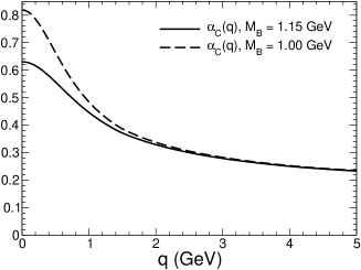
In Fig. 1 we give two curves for the compound $\alpha_{\rm B}(q^{2})$, with almost the same parameters $\Lambda_{\rm V}$ from Eqs. (18) and (19), but significantly different frozen couplings owing to the change of the IR regulator by $15\%$. Later, for a comparison we shall also use the set with a smaller $\Lambda(n_{f}=3)=465$ MeV,

$$\Lambda_{V}(n_{f}=5)=292~{}{\rm MeV},~{}~{}\Lambda_{V}(n_{f}=4)=406~{}{\rm MeV},~{}~{}\Lambda(n_{f}=3)=465~{}{\rm MeV},$$ (20)

and a smaller $\alpha_{\rm crit}(q^{2}=0,n_{f}=3)=0.5712$.

Notice that the value of $\alpha_{\rm crit}=0.57$ is close to those which were used in phenomenology ref.2 ; ref.3 ; ref.4 ; ref.9 , with typical values $\alpha_{\rm crit}\sim 0.54-0.60$, but is significantly larger than the lattice $\alpha({\rm lat})\sim(0.22-0.30)$ in full QCD ref.14 ; ref.15 . The reason for that discrepancy possibly comes from lattice artifacts, present in the lattice GE potential ref.15 , and also from an additional normalization condition, usually put on the lattice static potential ref.27 ; ref.31 .

Also, in contrast to some lattice potentials, where saturation of the vector coupling takes place at very small distances, $r\sim 0.2$ fm ref.14 ; ref.15 , in our approach the vector coupling is approaching its critical value at the much larger distances $r\mathrel{\mathchoice{\lower 3.6pt\vbox{\halign{$\mathsurround=0pt\displaystyle\hfil#\hfil$\cr>\crcr\sim\crcr}}}{\lower 3.6pt\vbox{\halign{$\mathsurround=0pt\textstyle\hfil#\hfil$\cr>\crcr\sim\crcr}}}{\lower 3.6pt\vbox{\halign{$\mathsurround=0pt\scriptstyle\hfil#\hfil$\cr>\crcr\sim\crcr}}}{\lower 3.6pt\vbox{\halign{$\mathsurround=0pt\scriptscriptstyle\hfil#\hfil$\cr>\crcr\sim\crcr}}}}0.6$ fm (see Figs. 2,3).

From Eq. (17) it is evident that the asymptotic coupling $\alpha_{\rm crit}$ is fully determined by the ratio $\eta^{2}=\frac{M_{\rm B}}{\Lambda_{\rm V}^{2}}$ and in two-loop approximation is given by

$$\alpha_{\rm B}(q=0)=\frac{4\pi}{\beta_{0}t_{0}}\left(1-\frac{\beta_{1}}{\beta_{0}^{2}}\frac{\ln t_{0}}{t_{0}}\right),$$ (21)

with the logarithm

$$t_{0}=\ln\eta^{2}=\ln\left(\frac{M_{\rm B}^{2}}{\Lambda_{V}^{2}}\right).$$ (22)

It is clear that to determine the frozen coupling with great accuracy, one needs to exclude small uncertainties in the values of $\Lambda_{V}(n_{f}=3)$ and $M_{\rm B}$, which can change $\alpha_{\rm crit}(n_{f}=3)$ by $\sim 30\%$.

It is also important that the critical couplings in the momentum and the coordinate spaces coincide:

$$\alpha_{\rm B}({\rm crit})=\alpha_{\rm B}(r\to\infty)=\alpha_{\rm B}(q=0).$$ (23)

It is of interest to understand why in phenomenological models the smaller values $\Lambda_{V}(n_{f}=3)\sim 330-380$ MeV are often used (compared to those from Eq. (17)), giving, nevertheless, a good description of the low-lying meson states. Such values of $\Lambda_{V}$ correspond to a smaller $\Lambda_{\overline{\rm MS}}(n_{f}=3)\sim 250$ MeV, as compared to that from Eq. (4), and are close to those calculated in the quenched approximation on the lattice, $\Lambda(n_{f}=0)=(245\pm 20)$ MeV ref.32 . Nevertheless, in this case a reasonable agreement with experiment is also reached due to a smaller value taken for $M_{\rm B}$, so that the frozen constant is again large, $\alpha_{\rm B}(\rm crit)\sim 0.60$. Later we will show that the lattice results appear to be in a better agreement with ours, when the static force and the second derivative of the static potential are compared.

V The vector coupling in coordinate space

The vector coupling in the coordinate space is defined according to Eq. (3), where the integral can be rewritten in a different way, introducing the variable $y=\frac{q}{\Lambda_{V}}$,

$$\alpha_{\rm B}(r\Lambda_{V},\eta^{2})=\frac{2}{\pi}\int\limits_{0}^{\infty}dy\frac{\sin(r\Lambda_{V}y)}{y}\alpha_{\rm B}(y,\eta^{2}),$$ (24)

This expression explicitly shows that $\alpha_{\rm B}(r)$ depends on the combination $r\Lambda_{V}(n_{f})$, if $n_{f}$ is fixed, and also on the parameter $\eta^{2}=\frac{M_{\rm B}^{2}}{\Lambda_{V}(n_{f})^{2}}$.

Figure 2: Compound $\alpha_{\rm B}(r)$ with $\alpha_{\rm crit}=0.63015$ and the parameters from Eq. (18) (solid line), and $\alpha_{\rm B}(r)$ (dashed line) with $\alpha_{\rm crit}=0.819$ and the parameters from Eq. (19).

Figure 3: Comparison of the compound $\alpha_{\rm B}(r)$ with parameters from Eq. (18) and $\alpha_{\rm B}(r)$ with fixed $n_{f}=3$ and the same $\alpha_{\rm crit}$ and $\Lambda_{V}(n_{f}=3)=0.4974$ GeV.

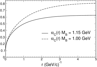
In Fig. 2 two couplings $\alpha_{\rm B}(r)$ are shown for two sets of $\Lambda(n_{f})$ from Eqs. (18), (19), where the critical values are equal to 0.630 ($M_{\rm B}=1.15$ GeV) and and 0.819 ($M_{\rm B}=1.0$ GeV).

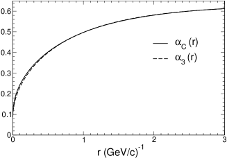
In Fig. 3 the calculated “compound” $\alpha_{\rm B}(r)$ with $M_{\rm B}=1.15$ GeV is compared to the coupling $\alpha_{\rm B}(r)$, in which $n_{f}=3$ is fixed (no matching), while for both couplings their critical values coincide and are equal to 0.630. As seen from Fig. 3, both curves are very close to each other and, perhaps just owing to this fact, the vector coupling with fixed $n_{f}=3$ may be used in phenomenological models. It also indicates that the frozen value of the coupling is of primary importance.

Notice that the situation is different for light and strange mesons, which have large sizes, and for them a screening of the GE interaction is possible, which can occur owing to open channels, decreasing the vector coupling.

VI The static force and the function $c(r)$

To have an additional test of the calculated vector coupling $\alpha_{\rm B}(r)$ we consider here the static force,

$$F_{\rm B}(r)=V_{\rm st}^{\prime}(r)=\sigma+V^{\prime}_{\rm GE}(r)\equiv\sigma+\frac{4}{3}\frac{\alpha_{\rm F}(r)}{r^{2}},$$ (25)

where the coupling

$$\alpha_{\rm F}(r)=\alpha_{\rm B}(r)-r\alpha^{\prime}_{\rm B}(r)$$ (26)

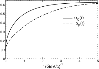
is introduced. The coupling $\alpha_{\rm F}(r)$ is smaller than $\alpha_{\rm B}(r)$, since the derivative $\alpha_{\rm B}^{\prime}(r)$ is positive. In Fig. 4 the coupling $\alpha_{\rm F}(r)$ together with $\alpha_{\rm B}(r)$ with parameters from Eq. (18) are plotted, which shows that $\alpha_{\rm F}(r)$ is smaller by $\sim 20\%$ in the region $0.5-0.6$ fm.

To compare our results with the existing lattice data we introduce the dimensionless function $r^{2}F_{\rm B}(r)$ and calculate two characteristic scales: $r_{1}$ and $r_{0}$ ref.33 :

$$r_{1}^{2}F_{\rm B}(r_{1})=1.0,\quad r_{0}^{2}F_{\rm B}(r_{0})=1.65,$$ (27)

where the function

$$r^{2}F_{\rm B}(r)=r^{2}\sigma+\frac{4}{3}\alpha_{\rm F}(r),$$ (28)

depends on both $\sigma$ and $\alpha_{\rm F}(r)$. For the static potential, like the Cornell and some lattice potentials, with the coupling equal to a constant, one has $\tilde{V}_{\rm st}(r)=\sigma r-\frac{e}{r}$ (where $e=\frac{4}{3}\alpha_{\rm lat}=constant$) and therefore in the static force,

$$\tilde{F}(r)=\sigma+\frac{e}{r^{2}},$$ (29)

the coupling $\alpha_{\rm F}=\frac{3}{4}e$ is also constant.

On the contrary, in our calculations the coupling $\alpha_{\rm F}(r)$ changes rapidly in the region $0\leq r\leq 0.4$ fm, approaching $\alpha_{\rm B}(r)$ only at large distances $r\geq 0.8$ fm (see Fig. 4, where $\Lambda_{V}(n_{f})$ is taken from Eq. (18) with $M_{\rm B}=1.15$ GeV).

Figure 4: The compound $\alpha_{\rm F}(r)$ and $\alpha_{\rm B}(r)$, taking $\Lambda_{\rm V}(n_{f})$ from Eq. (18) with $M_{\rm B}=1.15$ GeV, $\Lambda_{\rm V}(n_{f}=3)=0.4974$ GeV, and $\alpha_{{\rm B}~{}{\rm crit}}=0.63015$.

With the use of Eq. (27) one easily calculates the characteristic sizes:

$$r_{1}=1.530~{}{\rm GeV}^{-1}=0.303~{}{\rm fm},\quad r_{0}=2.321~{}{\rm GeV}^{-1}=0.460~{}{\rm fm},$$ (30)

taking $\Lambda_{\rm V}(n_{f}=3)=497.4$ MeV, which corresponds to the central value of the perturbative $\Lambda_{\overline{\rm MS}}(n_{f}=3)=337$ MeV. These numbers appear to be very close to those calculated on the lattice: $r_{1}({\rm lat})=1.621~{}$GeV${}^{-1}=0.321$ fm ref.34 and $r_{0}=1.3656(20)$ GeV${}^{-1}=(0.468\pm 0.004)$ fm ref.27 , being only several percent smaller. However, to reach precise agreement with the lattice scales one needs to take a bit smaller $\Lambda_{\overline{\rm MS}}(n_{f})$, namely, those values which correspond to the lower bounds in pQCD (4): $\Lambda_{\overline{\rm MS}}(n_{f}=5,2-{\rm loop})=208$ MeV, $\Lambda_{\overline{\rm MS}}(n_{f}=4)=279.2$ MeV, $\Lambda_{\overline{\rm MS}}(n_{f}=3)=322$ MeV. For this choice we have obtained $\alpha_{\rm crit}=0.5712$, $r_{1}=0.312$ fm, and $r_{0}=0.470$ fm, which coincide with the lattice scales from Refs. ref.34 ; ref.35 with an accuracy better than $3\%$.

In the cases considered, we have found the following values for the product $r_{0}~{}\Lambda_{\overline{\rm MS}}(n_{f}=3)$:

$$r_{0}~{}\Lambda_{\overline{\rm MS}}(n_{f}=3) = 0.764,~{}~{}{\rm for}~{}~{}r_{0}=0.470~{}{\rm fm},~{}~{}\alpha_{\rm crit}=0.5712,$$

$$r_{0}~{}\Lambda_{\overline{\rm MS}}(n_{f}=3) = 0.782,~{}~{}{\rm for}~{}~{}r_{0}=0.460~{}{\rm fm},~{}~{}\alpha_{\rm crit}=0.630,$$ (31)

in good agreement with the lattice results from Refs. ref.27 ; ref.34 . Thus we conclude that for large $\Lambda_{\rm V}(n_{f}=3)\sim 500$ MeV, with the corresponding $\Lambda_{\overline{\rm MS}}=0.339$ MeV, one needs to take a relatively large IR regulator $M_{\rm B}=1.15$ GeV to obtain the scales $r_{1},~{}r_{0}$ in agreement with the lattice results. For a smaller regulator, e.g. $M_{\rm B}=1.0$ GeV, the scales $r_{1},~{}r_{0}$ turn out to be smaller: $r_{1}=0.292$ fm, $r_{0}=0.442$ fm, giving $r_{0}~{}\Lambda_{\overline{\rm MS}}(n_{f}=3)=0.757$. On the contrary, the large value $r_{0}=0.50$ fm may be obtained in two ways: either with the larger regulator $M_{\rm B}\mathrel{\mathchoice{\lower 3.6pt\vbox{\halign{$\mathsurround=0pt\displaystyle\hfil#\hfil$\cr>\crcr\sim\crcr}}}{\lower 3.6pt\vbox{\halign{$\mathsurround=0pt\textstyle\hfil#\hfil$\cr>\crcr\sim\crcr}}}{\lower 3.6pt\vbox{\halign{$\mathsurround=0pt\scriptstyle\hfil#\hfil$\cr>\crcr\sim\crcr}}}{\lower 3.6pt\vbox{\halign{$\mathsurround=0pt\scriptscriptstyle\hfil#\hfil$\cr>\crcr\sim\crcr}}}}1.30$ GeV, if the “perturbative” $\Lambda_{\overline{\rm MS}}(n_{f}=3)$ from Eq. (4) is used, or taking the significantly smaller value of $\Lambda_{\overline{\rm MS}}(n_{f}=3)\sim 245$ MeV, as in the quenched calculations ref.32 . Thus we can conclude that the scale $r_{0}$ cannot be considered as a universal parameter but depends on which values of $\Lambda$ and $M_{\rm B}$ are used. Notice, that the force $F_{\rm B}(r)$ depends also on the string tension and our calculations with $\sigma=0.18$ GeV² give the scales $r_{1}$ and $r_{0}$ in good agreement with the lattice results.

An additional and very important test of the vector coupling comes from the study of the function $c(r)$, which is defined via the second derivative of the static potential and therefore does not depend on the string tension. It is determined by $\alpha_{\rm B}(r)$ and its first and second derivatives:

$$c(r)=\frac{1}{2}r^{3}~{}V_{\rm st}^{\prime\prime}(r)=-\frac{4}{3}\alpha_{\rm F}(r)-\frac{4}{3}\alpha_{\rm{\rm B}}^{\prime\prime}(r)\frac{r^{2}}{2}.$$ (32)

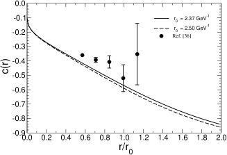
The second derivative $\alpha_{\rm B}^{\prime\prime}(r)$ is negative and therefore the magnitude of $c(r)$ appears to be smaller than that of $\frac{4}{3}\alpha_{\rm F}(r)$. Moreover, the slope of $c(r)$ depends on the IR regulator used. The behavior of $c(r)$ in our case, with $n_{f}=3$, is shown in Fig. 5 together with the points taken from the lattice calculations of the ALPHA group, with $n_{f}=2$ ref.36 (unfortunately, we could not find any lattice data in full QCD). From Fig. 5 one can see a qualitative agreement with both results.

Figure 5: The function $c(r)$ for $M_{\rm B}=1.15$ GeV and $\Lambda_{V}(n_{f})$ from Eq. (18); the points with the errors are taken from Ref. ref.36 , where the function $c(r)$ was calculated on the lattice with $n_{f}=2$.

VII The bottomonium spectrum as a test of $\alpha_{\rm crit}$

In bottomonium the centroid mass $\bar{M}(nl)$ for a given multiplet $nl$ just coincides with the eigenvalue $\bar{M}(nl)$ of the Hamiltonian given in Eq. (8):

$$\left[2\sqrt{\bm{p}^{2}+m_{b}^{2}}+V_{\rm st}(r)\right]\varphi_{nl}=\bar{M}(nl)\varphi_{nl}.$$ (33)

Our present calculations using the SSE (the relativistic case) have better accuracy than in the nonrelativistic and so-called einbein approximations, although the differences between them are only $\sim 10$ MeV for low-lying masses $\bar{M}(nl)$ and their mass splittings.

The bottomonium spectrum was calculated taking the compound $\alpha_{\rm B}(r)$ with the values of $\Lambda_{\rm V}(n_{f})$ from (18) and also in the case with fixed $n_{f}=3$ and the same $\Lambda_{\rm V}(n_{f}=3)=497.4$ MeV, but without matching. It appears that in these two cases the differences between the masses calculated are very small, $\sim 2-6$  MeV. Therefore it is of special importance to calculate the spectrum, considering a different $\Lambda_{\rm V}$ for $n_{f}=3$, or a different $\Lambda_{\overline{\rm MS}}(n_{f}=3)$. Our calculations show that there are several mass splittings, which are most sensitive to the choice of the ratio $\eta^{2}=\frac{M_{\rm B}^{2}}{\Lambda_{\rm V}^{2}}$, determining the frozen value of $\alpha_{\rm B}(r)$. Their experimental values are taken from Refs. ref.18 ; ref.37 ; ref.38 :

$$\bar{M}(2P)-\bar{M}(1P) = (360.0\pm 1.7)~{}{\rm MeV},$$

$$\bar{M}(3P)-\bar{M}(2P) = (280\pm 14)~{}{\rm MeV},$$

$$\bar{M}(1D)-\bar{M}(1P) = (264\pm 2)~{}{\rm MeV}.$$ (34)

Here the centroid mass $\bar{M}(\chi_{b}(3P))\simeq(10540\pm 5)$ MeV is estimated from two experimental masses measured by the ATLAS ref.37 and the D0 ref.38 collaborations.

In Ref. ref.13 it was already demonstrated that the fit to the bottomonium splittings appears to be sensitive to the choice of the critical coupling constant. However, in the vector coupling the parameters were often taken in a rather arbitrary way. In particular, for the lattice static potential with small $\alpha_{\rm lat}(r)=const=0.306$ ($n_{f}=3$) the $1D-1P$ and $1P-1S$ splittings are by $40-30$ MeV smaller than their experimental values.

Here, we first determine the masses of the $1D$ multiplet. The fine-structure splittings of this multiplet were calculated taking the strong coupling in the spin-orbit and tensor interactions close to the value for the $1P$-states ref.30 , namely, $\alpha_{\rm FS}(\mu_{\rm FS})=0.40$ at the scale $\mu_{\rm FS}\sim 1$ GeV. We take the spin-orbit splitting $a(1D)$ and tensor splitting $t(1D)$ in one-loop approximation ref.39 :

$$a(nl)=\frac{2\alpha_{\rm FS}}{\omega(nl)^{2}}\langle r^{-3}\rangle_{nl}-\frac{\sigma}{2\omega(nl)^{2}}\langle r^{-1}\rangle_{nl},\quad c(nl)=\frac{4\alpha_{\rm FS}}{3\omega(nl)^{2}}\langle r^{-3}\rangle_{nl},$$ (35)

where in the denominator, instead of the quark mass usually used ref.40 , one has to put the quark kinetic energy. This result follows from the analysis of the spin-dependent part of the RSH $H_{\rm R}$ in Ref. ref.39 . For the $1D$ states the calculated kinetic energy is $\omega(1D)=5.0$ GeV. For the $1D$ states and the set of the parameters from Table 1 with $M_{\rm B}=1.15$ GeV, the following values of the matrix elements were calculated: $\langle r^{-3}\rangle_{\rm 1D}=0.132(2)$ GeV³ and $\langle r^{-1}\rangle_{\rm 1D}=0.444(4)$ GeV. Then the fine-structure splittings $a(1D)=2.6$ MeV and $c(1D)=2.8$ MeV were calculated. Then the masses of the $n\,^{3}D_{J}$ states are defined as in Ref. ref.40 ,

$$M(1\,^{3}D_{3}) = \bar{M}(1D)+2a-\frac{c}{7},$$

$$M(1\,^{3}D_{2}) = \bar{M}(1D)-~{}a+\frac{c}{2},$$

$$M(1\,^{3}D_{1}) = \bar{M}(1D)-3a-\frac{c}{2}.$$ (36)

Then taking from the experiments the centroid mass $\bar{M}(1D)=10164$ MeV (see below) and the values of $a$ and $c$, using Eq. (35), the following masses $M(n\,^{3}D_{J})$ are obtained:

$$M(1\,^{3}D_{3})=(10169\pm 2)~{}{\rm MeV},$$

$$M(1\,^{3}D_{2})=(10163\pm 2)~{}{\rm MeV},$$

$$M(1\,3D_{1})=(10155\pm 2)~{}{\rm MeV}.$$ (37)

The centroid mass used, according to (36), is by $\sim 1$ MeV larger than $M(1\,^{3}D_{2})=(10163\pm 2)$ MeV, known from experiments, i.e., $\bar{M}(1D)=(10164\pm 2)$ MeV. From Eq. (37) our calculations give the splittings of the $1D$ multiplet: $M(1\,^{3}D_{3})-M(1\,^{3}D_{1})=14(4)$ MeV and $M(1\,^{3}D_{2})-M(1\,^{3}D_{1})=8(4)$ MeV, which appear to be two times smaller than those obtained in lattice calculations ref.41 .

For the $nP$ bottomonium multiplets their spin-averaged masses are known very accurately ref.18 ; ref.42 ; ref.43 :

$$\bar{M}(1P)=(9900.0\pm 0.6)~{}{\rm MeV},\quad\bar{M}(2P)=(10260\pm 0.7)~{}{\rm MeV},$$ (38)

and therefore their mass splitting $\bar{M}(2P)-\bar{M}(1P)=260(2)$ MeV is also known with great accuracy and may be used as a test of different sets of the parameters.

Table 1: The mass splittings in bottomonium in MeV ($\Lambda_{\overline{\rm MS}}(n=3)=325$ MeV)

	$M_{\rm B}=1.15$ GeV	$M_{\rm B}=1.10$ GeV	exp. ref.18
State	$m_{b}=4.832$ GeV	$m_{b}=4.840$ GeV
$1D-1P$	259	261	$264\pm 2$
$2P-1P$	371	376	$360\pm 2$
$3P-2P$	288	294	$280\pm 14$

As seen from Table 1, the $1D-1P$ splitting is in good agreement with experiment for $M_{\rm B}=1.10$ GeV, however, at the same time the $2P-1P$ splitting increases with decreasing $M_{\rm B}$ and one needs to reach the best agreement for both splittings. Choosing different sets of the parameters $M_{\rm B}$ and $\Lambda_{V}(n=3)$, we have observed that a good agreement with the experimental splittings takes place for the frozen constant $\alpha_{\rm crit}=0.57\pm 0.02$ and the IR regulator $M_{\rm B}=(1.15\pm 0.02)$ GeV, while the calculated spin-averaged masses coincide with experiment within $\pm(5-10)$ MeV. Notice, that the lattice calculations give larger $D$-wave masses ref.41 , as compared to ours, while smaller masses $M(1D)$ were predicted in Ref. ref.40 .

For the $2P-1P$ splitting a small deviation $\sim 5$ MeV from the experimental value can be obtained, if a smaller QCD constant $\Lambda_{\overline{\rm MS}}(n=3)=(317\pm 5)$ MeV is used, while $M_{\rm B}=(1.15\pm 0.02)$ GeV is relatively large.

We do not give here the centroid masses of the $S$-states, because for calculations of $\bar{M}(1S),~{}\bar{M}(2S)$ one needs to take into account the nonlinear behavior of the confining potential at short distances, $r\lower 3.01385pt\hbox{$\;\stackrel{{\scriptstyle\textstyle<}}{{\sim}}\;$}0.20$ fm, and this fact gives rise to an additional uncertainty – small negative corrections to the $S$-wave masses. Such corrections are very small for the states with $l\neq 0$, since their w.f.s are equal to zero near the origin, while the $S$-wave w.f.s have their maximum values there.

VIII Conclusions

We have studied the vector coupling in the momentum and coordinate spaces, introducing the IR regulator, $M_{\rm B}=\sqrt{2\pi\sigma}=(1.06\pm 0.11)$ GeV, as it is prescribed in BPT.

For the vector coupling in momentum space we have performed the matching procedure at the quark mass thresholds and calculated the “vector” constants $\Lambda_{\rm V}(n_{f})$. It appears that these constants correspond to $\Lambda_{\overline{\rm MS}}(n_{f})$, which coincide with the perturbative $\Lambda_{\overline{\rm MS}}(n_{f})$ within $\pm 5$ MeV. Moreover, their values weakly depend on the regulator $M_{\rm B}$, if it is taken from the range $(1.0-1.20)$ GeV. We have shown that in the static force the scales $r_{0}$ and $r_{1}$ are not universal numbers and depend on the IR regulator used. Thus $r_{0}$ decreases by $6\%$ when $M_{\rm B}$ decreases from the value $M_{\rm B}=1.15$ GeV to $M_{\rm B}=1.00$ GeV.

The ratio $\frac{r_{0}}{r_{1}}=1.505\pm 0.02$ and the product $r_{0}\Lambda_{\overline{\rm MS}}(n_{f}=3)=0.77\pm 0.02$ were calculated. The choice with $M_{\rm B}=1.15$ GeV and $\Lambda_{\overline{\rm MS}}(n_{f}=3)=322$ MeV gives the best (precise) agreement with the lattice scales $r_{0}$ and $r_{1}$. The function $c(r)$, which is proportional to the second derivative of the static potential and does not depend on the string tension, is calculated. This function illustrates that the saturation of the vector coupling takes place at the distances $r\mathrel{\mathchoice{\lower 3.6pt\vbox{\halign{$\mathsurround=0pt\displaystyle\hfil#\hfil$\cr>\crcr\sim\crcr}}}{\lower 3.6pt\vbox{\halign{$\mathsurround=0pt\textstyle\hfil#\hfil$\cr>\crcr\sim\crcr}}}{\lower 3.6pt\vbox{\halign{$\mathsurround=0pt\scriptstyle\hfil#\hfil$\cr>\crcr\sim\crcr}}}{\lower 3.6pt\vbox{\halign{$\mathsurround=0pt\scriptscriptstyle\hfil#\hfil$\cr>\crcr\sim\crcr}}}}0.6$ fm.

Our analysis of the bottomonium spectrum shows that the splittings $\bar{M}(1D)-\bar{M}(1P)$ and $\bar{M}(2P)-\bar{M}(1P)$ are very sensitive to the factor $\eta^{2}=\frac{M_{\rm B}^{2}}{\Lambda_{\rm V}(n_{f}=3)^{2}}$ and the best agreement with experiment is reached taking $\eta=2.46\pm 0.04$. We have derived the value of the frozen coupling: $\alpha_{\rm crit}=0.57\pm 0.02$. The following splittings for the members of the bottomonium $1D$ multiplet are predicted: $M(1\,^{3}D_{3})-M(1\,^{3}D_{1})=14(2)$ MeV,  $M(1\,^{3}D_{2})-M(1\,^{3}D_{1})=8(2)$ MeV.