Convergence rate of Markov chain methods for genomic motif discovery

Abstract

We analyze the convergence rate of a simplified version of a popular Gibbs sampling method used for statistical discovery of gene regulatory binding motifs in DNA sequences. This sampler satisfies a very strong form of ergodicity (uniform). However, we show that, due to multimodality of the posterior distribution, the rate of convergence often decreases exponentially as a function of the length of the DNA sequence. Specifically, we show that this occurs whenever there is more than one true repeating pattern in the data. In practice there are typically multiple such patterns in biological data, the goal being to detect the most well-conserved and frequently-occurring of these. Our findings match empirical results, in which the motif-discovery Gibbs sampler has exhibited such poor convergence that it is used only for finding modes of the posterior distribution (candidate motifs) rather than for obtaining samples from that distribution. Ours are some of the first meaningful bounds on the convergence rate of a Markov chain method for sampling from a multimodal posterior distribution, as a function of statistical quantities like the number of observations.

T1Supported in part by U.S. NSF awards CMMI-0926814 and DMS-12-09103 and by NSERC of Canada.

and

1 Introduction

Gene regulatory binding motifs are short DNA sequences that control gene expression. The identification of these regulatory motifs poses several challenges: they are only 6–15 base pairs in length, and do not contain clear start and stop codons; a regulatory motif is indistinguishable from random sequences of the same length except that it is a particular sequence that occurs more frequently than expected under the background model. Discovery of previously undescribed regulatory motifs in DNA sequences thus involves both finding such a repeating pattern (“motif”) and determining where that pattern occurs in the sequences [Kellis et al. (2004)]; this is illustrated in Figure 1.

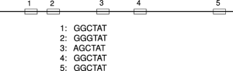
Figure 1: Illustration of motif discovery: finding an unknown repeating pattern in a long DNA sequence. The pattern can vary slightly between instances.

One of the most effective methods for identifying new regulatory motifs is based on a statistical model and associated Gibbs sampling computational method [Liu, Neuwald and Lawrence (1995)]. This approach has been popularized with the availability of software programs for its use, such as BioProspector [Liu, Brutlag and Liu (2001)] and AlignAce [Roth et al. (1998)].

Like most other methods for identifying regulatory motifs, the Gibbs sampling method often yields different answers when starting from different initial configurations. The method is applied by rerunning the Gibbs sampler many times, using randomly generated initial positions. The resulting candidate motifs are sorted according to some goodness-of-fit measure, and then the highest-scoring motifs are reported [Lawrence et al. (1993), Liu, Brutlag and Liu (2001), Jensen et al. (2004)]. This fact contrasts with the theoretical properties and traditional use of a Gibbs sampler, namely to be simulated until it has some claim of having converged to the posterior distribution, at which point the answer should be the same regardless of initialization.

We address a particular model and Gibbs sampler that are representative of this family of methods. We analyze the convergence rate of a simplified version of the Gibbs sampler and show that, due to multimodality of the posterior distribution, the convergence rate typically decreases exponentially as a function of the DNA sequence length (Theorem 3.2). Specifically this occurs when there is more than one true repeating pattern in the data, meaning that the DNA is made up of short subsequences, each of which is either equal to one of several motifs or is generated from the background model. In practice there are typically multiple distinct repeating patterns in biological data, corresponding to multiple gene regulatory binding motifs or to repeating patterns that have other biological significance, such as “determinants of mRNA stability or even sites for regulation by antisense transcripts” [Roth et al. (1998)]. The goal is to detect the most frequently-occurring and well-conserved motif or motifs [Neuwald, Liu and Lawrence (1995)]. So in practice we can expect the sampler convergence rate to decay exponentially; this is equivalent to the run time of the algorithm growing exponentially in the sequence length, for a fixed accuracy. The multimodality of the posterior and resulting poor convergence are illustrated in Figure 2, which shows posterior density estimates of a particular function of the parameter vector, from two different Gibbs sampling chains. Initialized with distinct parameter values, the two chains have become trapped in different modes of the posterior density and thus have not yet individually converged to the posterior distribution.

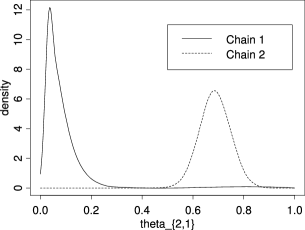
Figure 2: The posterior density estimates of $\hat{\theta}_{2,1}(\mathbf{A})$ from two different Gibbs sampling chains, in the case of two true motifs.

The multimodality of the posterior distribution arises due to a contradiction between the data, which typically have multiple true repeating patterns, and the model assumption of a single such pattern. Practitioners use the model not because it is believed to precisely capture the true process that generated the data (which is extremely complex) but because it captures several important features of that process [Neuwald, Liu and Lawrence (1995), Roth et al. (1998)]. Our results show that the presence of multiple motifs, even if some occur very infrequently, causes slow convergence. Recognizing that there can be multiple true motifs, a variant on the Gibbs sampler has been proposed that allows for a fixed number of motifs greater than one [Neuwald, Liu and Lawrence (1995)]. This approach is only likely to fix the slow convergence if the number of motifs in the model is at least as large as the number of true motifs in the data. This is only a practical solution if the number of true motifs is small.

Our simplification of the model and associated Gibbs sampler assumes that motifs can only end at locations in the sequence that are divisible by the motif length, instead of at arbitrary locations (Section 2.2). This is done to facilitate analysis, by avoiding the “phase shift” issue that occurs in the original sampler [Lawrence et al. (1993), Liu (1994)]. Since phase shift slows convergence of the chain, it is likely (but unproven) that our results on slow convergence of the simplified chain also hold for the original chain.

We also give evidence supporting the conjecture that the convergence rate decreases polynomially if there is no more than one true (and identifiable) motif in the data. We give empirical evidence, and prove polynomial decay of the convergence rate for the case of length-one motifs. In this case any true motifs are nonidentifiable; see Theorem 3.3.

Ours are some of the few meaningful bounds on the convergence rate of a Markov chain method used in Bayesian statistics, as a function of statistical quantities such as the number of observations or number of groups. Such results are particularly rare for multimodal posterior densities. Roberts and Sahu (2001) show that the convergence rate of a Gibbs sampler for a unimodal posterior density in $\mathbb{R}^{d}$ approaches a constant as the number of observations increases. Belloni and Chernozhukov (2009) show that if the posterior density converges uniformly to a normal density, then a Metropolis–Hastings chain restricted to a neighborhood of the true parameter value has polynomially decaying convergence rate. Jones and Hobert (2001, 2004) and other authors [e.g., Rosenthal (1995, 1996)] obtain bounds on the time to be within distance $\varepsilon>0$ of convergence for various hierarchical random effect models having unimodal posterior densities, as a function of the initial values, data and hyperparameters. Mossel and Vigoda (2006) show that the convergence rate of a Markov chain method used in Bayesian phylogenetics can decrease exponentially in the number of samples in the dataset. We also learned after completing this article that Dr. Scott Schmidler at Duke University has independently obtained some convergence results in the motif-discovery context (personal communication).

Showing that a Markov chain method used in statistical practice is “well-behaved” usually consists of proving geometric ergodicity [Liu, Wong and Kong (1995), Jarner and Hansen (2000), Fort et al. (2003), Johnson and Jones (2010)], meaning that the chain converges to the posterior distribution at a geometric rate. The Gibbs sampler we analyze satisfies the even stronger property of uniform ergodicity; despite this, it is so poorly-behaved as to be unusable for obtaining samples from the posterior distribution for long DNA sequences.

Characterizing the dependence of the convergence rate on statistical quantities like the number of observations or the number of parameters is critical in justifying the use of a Markov chain method. However, there are several difficulties in doing so. First, the posterior distribution of a statistical model has a much more complex form than the stylized distributions for which Markov chain convergence rates are typically obtained [Borgs et al. (1999), Bhatnagar and Randall (2004), Woodard, Schmidler and Huber (2009b)]. Second, the data, and thus the convergence rate of the Markov chain, are stochastic and depend on the data-generating mechanism.

We address these challenges by utilizing Bayesian asymptotic theory, which characterizes the behavior of the posterior distribution as the number of observations grows. This is complicated by the fact that Bayesian asymptotic theory is most well developed in the case of a continuous parameter space, but the motif Gibbs sampler is defined on a discrete parameter space. We handle this by applying the asymptotic results on an alternative continuous parameterization of the motif model and then mapping those results to the discrete parameterization. Due to these technical challenges our main theorem requires sufficiently long motifs, and is restricted to the case where each true motif corresponds to a fixed sequence of nucleotides (disallowing the small variations seen in Figure 1). We give an additional argument and simulation results suggesting that slow mixing holds even for very short motifs, and when the true motifs are allowed to vary between instances.

The motif discovery example provides insights into the dynamics of standard Markov chain methods applied to statistical models with highly multimodal posterior distributions. Other examples that may have the same exponential-time property include Markov chains for model search in the context of regression with a large number of predictors [Liang and Wong (2000), Hans, Dobra and West (2007)] and Markov chains for spatial mixture models based on random fields [Geman and Geman (1984), Green and Richardson (2002)]. Our example also provides a test case for the use of more sophisticated Markov chain methods that are designed to handle multimodality [Del Moral, Doucet and Jasra (2006), Andrieu, Doucet and Holenstein (2010)]: if a method can be shown to sample from the posterior distribution of the motif-discovery model in polynomial time, then it would be dramatically more efficient than the Gibbs sampling approach.

Background on the Gibbs sampling method for motif discovery and on Markov chain convergence rates is in Section 2. Our convergence results are in Section 3, and a simulation study is given in Section 4. The proof of our main result is in Section 5, and we draw conclusions in Section 6.

2 Background

2.1 Statistical motif discovery

The goal of motif discovery is to find short sub-sequences of nucleotides (length 6–15 base pairs) that occur multiple times (more often than could be explained under the background model) in one or more long DNA sequences. Neither the nucleotide pattern nor the sub-sequence locations are known. This goal is illustrated in Figure 1.

We address one of the two main variants of Gibbs sampler used in motif discovery. The variant we analyze takes the number of motif instances per sequence to be unknown, while the other variant fixes the number of instances per sequence [Jensen et al. (2004)]; the two approaches are closely related and should have similar properties. Programs such as BioProspector are based on the method we analyze, and build in a number of additional features, such as a prior distribution on the motif frequency and handling of gapped motifs; however, by adding parameters and complexity to the model these enhancements probably make the Gibbs sampler slower to converge, and so are unlikely to affect our slow-mixing results.

We focus further on the case of a single DNA sequence (having an unknown number of motif instances). The case of multiple sequences can be addressed by concatenating to obtain a single sequence.

The motif instances are not necessarily identical. Taking the length $w$ of the motif to be known, one can describe the nucleotide pattern by a position-specific frequency matrix, which contains the probability of occurrence of each nucleotide at each position in the motif. Call this matrix $\bolds{\theta}_{1:w}=(\bolds{\theta}_{1},\ldots,\bolds{\theta}_{w})$, where $\bolds{\theta}_{k}$ is the unknown probability vector for the $k$th position. Let the nucleotides be labeled $1,\ldots,M$, so that $\bolds{\theta}_{k}$ has length $M$; for DNA data $M=4$. For each instance of the motif, the nucleotide in position $k$ is assumed to be drawn independently from a discrete distribution with parameters $\bolds{\theta}_{k}$. The positions in the full sequence that are not part of a motif instance are assumed to have nucleotide drawn independently from a discrete distribution with unknown probability vector $\bolds{\theta}_{0}$.

Let $\mathbf{S}=(S_{1},\ldots,S_{L})\in\{1,\ldots,M\}^{L}$ be the observed sequence, havinglength $L$. In the original model of, for example, Liu, Neuwald and Lawrence (1995), a motif is allowed to start at any index $i\in\{1,\ldots,L-w+1\}$, but we will analyze a simplified version that only allows a motif to start at indices $wi-w+1$ for $i\in\{1,\ldots,L/w\}$ where $L$ is divisible by $w$. This choice is explained in Section 2.2. Let $A_{i}\in\{0,1\}$ be the (unknown) indicator of whether a motif begins at index $wi-w+1$, for $i\in\{1,\ldots,L/w\}$, and define $\mathbf{A}=(A_{1},\ldots,A_{L/w})$. Let $\mathbf{N}(\mathbf{A}^{(k)})$ be the length-$M$ vector of counts of the occurrence of each nucleotide at position $k\in\{1,\ldots,w\}$ of all motif instances, conditional on $\mathbf{A}$. Similarly, $\mathbf{N}(\mathbf{A}^{c})$ is defined to be the length-$M$ vector of counts for each nucleotide in the background locations, that is, the locations that are not part of any motif instance,

$$\qquad N\bigl{(}\mathbf{A}^{(k)}\bigr{)}_{m} \triangleq \sum_{i=1}^{L/w}\mathbf{1}_{\{A_{i}=1,S_{wi-w+k}=m\}},\qquad k\in\{1,\ldots,w\},m\in\{1,\ldots,M\},$$

$$N\bigl{(}\mathbf{A}^{c}\bigr{)}_{m} \triangleq N(\mathbf{S})_{m}-\sum_{k=1}^{w}N\bigl{(}\mathbf{A}^{(k)}\bigr{)}_{m},$$ (1)

$$N(\mathbf{S})_{m} \triangleq \sum_{i=1}^{L}\mathbf{1}_{\{S_{i}=m\}}.$$

For any two equal-length vectors $\bolds{\beta}=(\beta_{1},\ldots,\beta_{K})$ and $\mathbf{n}=(n_{1},\ldots,n_{K})$ define the notation

$$\bolds{\beta}^{\mathbf{n}}=\prod_{k=1}^{K}\beta_{k}^{n_{k}},\qquad\Gamma(\mathbf{n})=\prod_{k=1}^{K}\Gamma(n_{k}),\qquad|\mathbf{n}|=\sum_{k=1}^{K}n_{k},$$ (2)

where $\Gamma$ is the gamma function. Using this notation, the likelihood conditional on $\mathbf{A}$ can be written as

$$\pi(\mathbf{S}|\mathbf{A},\bolds{\theta}_{0:w}) = \prod_{i=1}^{L/w}\Biggl{[}\prod_{k=1}^{w}\theta_{k,S_{wi-w+k}}\Biggr{]}^{\mathbf{1}_{\{A_{i}=1\}}}\Biggl{[}\prod_{k=1}^{w}\theta_{0,S_{wi-w+k}}\Biggr{]}^{\mathbf{1}_{\{A_{i}=0\}}}$$

$$= \bolds{\theta}_{0}^{\mathbf{N}(\mathbf{A}^{c})}\times\prod_{k=1}^{w}\bolds{\theta}_{k}^{\mathbf{N}(\mathbf{A}^{(k)})},$$

where $\bolds{\theta}_{0:w}=(\bolds{\theta}_{0},\bolds{\theta}_{1},\ldots,\bolds{\theta}_{w})$ denotes all model parameters. We will use $\pi$ to indicate the likelihood, prior or the full, marginal or conditional posterior distributions as distinguished by its arguments.

The prior distributions for the unknown quantities are $\pi(\bolds{\theta}_{k})=\operatorname{Dirichlet}(\bolds{\beta}_{k})$ for $k\in\{0,\ldots,w\}$ and $\pi(A_{i}=1)=p_{0}$ independently. Here $p_{0}\in(0,1)$ is a known constant and $\bolds{\beta}_{0},\ldots,\bolds{\beta}_{w}$ are fixed length-$M$ vectors with $\beta_{k,m}>0$. The corresponding posterior distribution is [Jensen et al. (2004)]

$$\pi(\mathbf{A},\bolds{\theta}_{0:w}|\mathbf{S})\propto\pi(\mathbf{A},\bolds{\theta}_{0:w},\mathbf{S})$$

(4)

$$\qquad=p_{0}^{|\mathbf{A}|}(1-p_{0})^{L/w-|\mathbf{A}|}\times\bolds{\theta}_{0}^{\mathbf{N}(\mathbf{A}^{c})+\bolds{\beta}_{0}-1}\times\prod_{k=1}^{w}\bolds{\theta}_{k}^{\mathbf{N}(\mathbf{A}^{(k)})+\bolds{\beta}_{k}-1}.$$

Liu, Neuwald and Lawrence (1995) integrate out the parameters $\bolds{\theta}_{0:w}$ in the above formula to yield a posterior distribution on $\mathbf{A}$. Using the notation from (2),

$$\pi(\mathbf{A}|\mathbf{S})$$

$$\qquad\propto p_{0}^{|\mathbf{A}|}(1-p_{0})^{L/w-|\mathbf{A}|}\frac{\Gamma(\mathbf{N}(\mathbf{A}^{c})+\bolds{\beta}_{0})}{\Gamma(|\mathbf{N}(\mathbf{A}^{c})|+|\bolds{\beta}_{0}|)}\prod_{k=1}^{w}\frac{\Gamma(\mathbf{N}(\mathbf{A}^{(k)})+\bolds{\beta}_{k})}{\Gamma(|\mathbf{N}(\mathbf{A}^{(k)})|+|\bolds{\beta}_{k}|)}.$$

Liu (1994) gives theoretical results supporting faster convergence of a Gibbs sampler for the reduced posterior $\pi(\mathbf{A}|\mathbf{S})$ relative to a Gibbs sampler for $\pi(\mathbf{A},\bolds{\theta}_{0:w}|\mathbf{S})$. So Liu, Neuwald and Lawrence (1995) propose to use a Gibbs sampler to draw from $\pi(\mathbf{A}|\mathbf{S})$, having state vector $\mathbf{A}\in\mathcal{X}\triangleq\{0,1\}^{L/w}$. This sampler iteratively updates each $A_{i}$ according to its conditional posterior distribution; details are given in Section 5.1.

Although this Gibbs sampler has both systematic-scan and random-scan versions, we expect that the mixing properties (defined in Section 2.3) of the two versions are identical. For this reason we focus attention on the random-scan Gibbs sampler, which is easier to analyze. We also make the transition matrix of the Markov chain nonnegative definite by including a holding probability of $1/2$ at every state; this is a common technique when analyzing the mixing properties of Markov chains [Madras and Zheng (2003), Woodard, Schmidler and Huber (2009a)]. It only increases the mixing time (Section 2.3) by a factor of two, so it does not affect results on the order of the run time as a function of $L$. Let $\mathbf{A}_{[-i]}$ indicate the vector $\mathbf{A}$ excluding the $i$th element, and $\pi(A_{i}|\mathbf{A}_{[-i]},\mathbf{S})\propto\pi(\mathbf{A}|\mathbf{S})$ indicate the conditional posterior distribution of $A_{i}$ given $\mathbf{A}_{[-i]}$. With these definitions we can write the transition matrix $T$ of the Gibbs sampler as follows for any $\mathbf{A},\mathbf{A}^{\prime}\in\mathcal{X}$:

$$T\bigl{(}\mathbf{A},\mathbf{A}^{\prime}\bigr{)} \triangleq \frac{1}{L/w}\sum_{i=1}^{L/w}\mathbf{1}_{\{\mathbf{A}^{\prime}_{[-i]}=\mathbf{A}_{[-i]}\}}$$

$$\hskip 41.0pt{}\times\frac{1}{2}\bigl{[}\mathbf{1}_{\{A_{i}^{\prime}=A_{i}\}}+\pi(A_{i}=0|\mathbf{A}_{[-i]},\mathbf{S})\mathbf{1}_{\{A_{i}^{\prime}=0\}}$$

$$\hskip 102.0pt{}+\pi(A_{i}=1|\mathbf{A}_{[-i]},\mathbf{S})\mathbf{1}_{\{A_{i}^{\prime}=1\}}\bigr{]}.$$

Expressions for $\pi(A_{i}|\mathbf{A}_{[-i]},\mathbf{S})$ are given in Section 5.1.

We also need an expression for the likelihood marginalized over $\mathbf{A}$. Using the vector notation $\mathbf{S}_{n:m}=(S_{n},\ldots,S_{m})$ for $n\leq m$,

$$\quad\pi(\mathbf{S}|\bolds{\theta}_{0:w}) = \prod_{i=1}^{L/w}f(\mathbf{S}_{wi-w+1:wi}|\bolds{\theta}_{0:w})\qquad\mbox{where}$$ (7)

$$f(\mathbf{s}|\bolds{\theta}_{0:w}) \triangleq p_{0}\prod_{k=1}^{w}\theta_{k,s_{k}}+(1-p_{0})\prod_{k=1}^{w}\theta_{0,s_{k}},\qquad\mathbf{s}\in\{1,\ldots,M\}^{w}.$$ (8)

Under model (7) and (8) each subsequence $\mathbf{S}_{wi-w+1:wi}$ is either generated from the motif $\bolds{\theta}_{1:w}$ with probability $p_{0}$, or generated from the background $\bolds{\theta}_{0}$ with probability $(1-p_{0})$. So we have i.i.d. observations $\mathbf{S}_{wi-w+1:wi}$ for $i\in\{1,\ldots,L/w\}$, which will allow us to use Bayesian asymptotic theory for i.i.d. parametric models.

2.2 Reason for the simplification

As stated in Section 2.1, while the original model allows a motif to start at any index $i\in\{1,\ldots,L-w+1\}$, we analyze a simplification of the model that assumes that motifs can only start at indices $wi-w+1$ for $i\in\{1,\ldots,L/w\}$. This simplification is done to facilitate analysis; however, we believe that our results are likely to hold for the original model as well.

First, our rapid mixing result (Theorem 3.3) immediately holds for the original model and associated Gibbs sampler. This is because it is for the case of $w=1$, where the original and simplified models are identical.

Second, the proof of our slow mixing result (Theorem 3.2) can be extended to the case where the model allows motifs to start at indices that are fixed distance $\geq w$ apart. However, Theorem 3.2 does not easily extend to the case where motifs can start in locations that are less than $w$ distance apart (including the original model). This is due to the following “phase shift” issue, which complicates analysis. For illustration consider the case where $M=4$ (there are four possible nucleotides) and $w=5$ (motifs are five nucleotides long), and the true motif is (deterministically) the sequence $(1,4,2,2,3)$. Phase shift means that it is possible to estimate that a motif begins or ends in the middle of one of the $(1,4,2,2,3)$ subsequences that exist in the data. For example, if the DNA sequence $\mathbf{S}$ satisfies $\mathbf{S}_{22:26}=(1,4,2,2,3)$, corresponding to a true motif beginning at position $22$, then the original model also allows for the possibility that $A_{23}=1$, meaning that a motif could be estimated to instead start at position $23$ with the sequence $4,2,2,3$.

While phase shift complicates analysis of the original Gibbs sampler, it should also make the original Gibbs sampler converge more slowly than the simplified Gibbs sampler. The effect of phase shift on convergence of the original Gibbs sampler is that it can become trapped in a local mode of the posterior distribution that corresponds to a shifted version of the true motif. This effect is described in Lawrence et al. (1993) and Liu (1994). To illustrate, take the above example where the true motif is $(1,4,2,2,3)$. There is a local mode of the posterior distribution for which the inferred motif starts with the sequence $4,2,2,3$, another for which the inferred motif ends with the sequence $1,4,2,2$, and so on. This posterior multimodality slows convergence of the original Gibbs sampler. It also suggests that our slow mixing result (Theorem 3.2) for the simplified Gibbs sampler holds for the original sampler.

Analysis of the original sampler should be possible using the same general approach taken here, but a number of the technical details would need to change. We leave this to future work.

2.3 Markov chain convergence rates

Consider a Markov chain with transition matrix $T$ and stationary distribution $\pi$ on a discrete state space $\mathcal{X}$. For $x\in\mathcal{X}$ and $D\subset\mathcal{X}$, let $T(x,D)=\sum_{y\in D}T(x,y)$. If the chain is initialized at $x\in\mathcal{X}$, then the total variation distance to stationarity after $n$ iterations is

$$\bigl{\|}T^{n}(x,\cdot)-\pi(\cdot)\bigr{\|}_{\mathrm{TV}}\triangleq\max_{D\subset\mathcal{X}}\bigl{|}T^{n}(x,D)-\pi(D)\bigr{|}.$$

The mixing time of the chain is the number of iterations required to be within distance $\varepsilon\in(0,1)$ of stationarity,

$$\tau_{\varepsilon}\triangleq\max_{x\in\mathcal{X}}\min\bigl{\{}n\dvtx\bigl{\|}T^{m}(x,\cdot)-\pi(\cdot)\bigr{\|}_{\mathrm{TV}}\leq\varepsilon\mbox{ for all }m\geq n\bigr{\}};$$

cf. Sinclair (1992).

Consider $T$ irreducible, aperiodic, reversible and nonnegative definite, which holds for the random-scan Gibbs sampler in Section 2.1. Then $\tau_{\varepsilon}$ is finite and closely related to the spectral gap $\operatorname{Gap}(T)\triangleq 1-\lambda_{2},$ where $\lambda_{2}\in[0,1)$ is the second-largest eigenvalue of $T$. Since the state space $\mathcal{X}$ is finite, $\operatorname{Gap}(T)>0$ and the chain is called uniformly ergodic [Roberts and Rosenthal (2004)]. The quantities $\tau_{\varepsilon}$ and $\operatorname{Gap}(T)$ are related via [Sinclair (1992)]

$$\tau_{\varepsilon} \leq \operatorname{Gap}(T)^{-1}\Bigl{(}-\ln\Bigl{[}\min_{x\in\mathcal{X}}\pi(x)\Bigr{]}-\ln\varepsilon\Bigr{)},$$

$$\tau_{\varepsilon} \geq \frac{1}{2}\bigl{(}1-\operatorname{Gap}(T)\bigr{)}\operatorname{Gap}(T)^{-1}\bigl{(}-\ln(2\varepsilon)\bigr{)}.$$

The efficiency of the Markov chain can be measured by how quickly $\tau_{\varepsilon}$ increases as a function of the problem difficulty, for instance the dimension of the parameter space. In our case we are interested in the dependence of $\tau_{\varepsilon}$ on the length $L$ of the DNA sequence, since in practice one analyzes very long sequences. We would certainly hope that $\tau_{\varepsilon}$ grows at most polynomially in $L$ for any fixed $\varepsilon$; this property is called rapid mixing. Slow mixing means that $\tau_{\varepsilon}$ increases exponentially for some $\varepsilon$. By (2.3) rapid mixing is equivalent to $\operatorname{Gap}(T)$ decreasing at most polynomially toward zero, and slow mixing is equivalent to $\operatorname{Gap}(T)$ decreasing exponentially toward zero, if $-\log[\min_{x\in\mathcal{X}}\pi(x)]$ increases polynomially in $L$. The latter property holds for the random-scan Gibbs sampler in Section 2.1. The rapid/slow mixing distinction is a measure of the computational tractability of an algorithm; polynomial factors are expected to be eventually dominated by increases in computing power due to Moore’s Law, while exponential factors cause a persistent computational problem.

3 Convergence results

We consider the mixing time (equivalently, spectral gap) of the Gibbs sampler when the data are drawn from a generalization of the model given in Section 2.1 that allows multiple true motifs. First we give negative results for the case of multiple true motifs, and then we give a positive result for a case with no true motifs.

3.1 Slow mixing for multiple true motifs

In this section, we show that if the data actually contain multiple true motifs, then the Gibbs sampler is slowly mixing: that $\operatorname{Gap}(T)$ is $\mathcal{O}(\alpha^{-L})$ for $\alpha>1$ where $-\log[\min_{x\in\mathcal{X}}\pi(x)]$ is $\mathcal{O}(L^{q})$ for some $q>0$. To make this statement precise in the presence of random data, we need to make assumptions about the model by which the data are generated. Our convergence results are obtained using Bayesian asymptotics based on this generative model; for other connections between Markov chain convergence and Bayesian asymptotics, see Kamatani (2011) and Belloni and Chernozhukov (2009).

For a concrete example to keep in mind, consider the case where $M=4$ (there are four possible nucleotides) and $w=5$ (motifs are five nucleotides long). Then let the DNA sequence $\mathbf{S}$ be generated as the concatenation of many length-five subsequences, each of which is either (motif one) equal to $(1,4,2,2,3)$ with probability 0.005, or (motif two) equal to $(4,2,4,1,3)$ with probability 0.001, or generated as i.i.d. noise where each nucleotide has equal probability. Theorem 3.2 below says that the Gibbs sampler $T$ is slowly mixing for data generated in this way.

When analyzing the Gibbs sampler we do not assume that the data $\mathbf{S}$ are generated according to the inference model (7) and (8). Our most general result only assumes that the subsequences $\mathbf{S}_{wi-w+1:wi}$ are i.i.d.

Assumption 3.1.

The data subsequences $\mathbf{S}_{wi-w+1:wi}$ indexed by $i\in\{1,\ldots,L/w\}$ are independent and identically distributed according to some probability mass function $g(\mathbf{s})>0\dvtx\mathbf{s}\in\{1,\ldots,M\}^{w}$, that is,

$$\mathbf{S}\sim\prod_{i=1}^{L/w}g(\mathbf{S}_{wi-w+1:wi}).$$

Under Assumption 3.1, we give a simple sufficient condition for slow mixing that relates the generative model $g(\mathbf{s})$ to the inference model $f(\mathbf{s}|\bolds{\theta}_{0:w})$ via the quantity $E\log f(\mathbf{s}|\bolds{\theta}_{0:w})=\sum_{\mathbf{s}}g(\mathbf{s})\log f(\mathbf{s}|\bolds{\theta}_{0:w})$. Since $\bolds{\theta}_{k}$ for $k\in\{0,\ldots,w\}$ is defined on the simplex $\Psi\triangleq\{\bolds{\theta}_{k}\dvtx\sum_{m=1}^{M}\theta_{k,m}=1,\theta_{k,m}\geq 0\}$, the quantity $E\log f(\mathbf{s}|\bolds{\theta}_{0:w})\in[-\infty,0)$ is a function of $\bolds{\theta}_{0:w}\in\Psi^{w+1}$. It is continuous in $\bolds{\theta}_{0:w}$, because it is a linear combination of a finite number of the continuous functions $\log f(\mathbf{s}|\bolds{\theta}_{0:w})$. We call $\eta(\bolds{\theta}_{0:w})\triangleq E\log f(\mathbf{s}|\bolds{\theta}_{0:w})$ multimodal if there exist $\bolds{\theta}^{(1)}_{0:w},\bolds{\theta}^{(2)}_{0:w}\in\Psi^{w+1}$ and bounded sets $F_{1}\ni\bolds{\theta}^{(1)}_{0:w}$ and $F_{2}\ni\bolds{\theta}^{(2)}_{0:w}$ such that

$$F_{1}\cap F_{2}=\varnothing\quad\mbox{and}\quad\sup_{\bolds{\theta}_{0:w}\in\partial F_{j}}\eta(\bolds{\theta}_{0:w})<\eta\bigl{(}\bolds{\theta}_{0:w}^{(j)}\bigr{)},\qquad j\in\{1,2\},$$ (10)

where $\partial F_{j}\triangleq\operatorname{cl}(F_{j})\cap\operatorname{cl}(F_{j}^{c})$ is the boundary of $F_{j}$. Equation (10) implies that $\bolds{\theta}^{(j)}_{0:w}$ is in the interior of $F_{j}$. For a continuous function on a closed, connected subset of $\mathbb{R}^{d}$ (like $\Psi^{w+1}$) this definition of multimodality is weaker than the existence of multiple strict local maxima and stronger than the existence of multiple local maxima. We call a function $h$ of $\bolds{\theta}_{0:w}$ a multiminimum function if $-h(\bolds{\theta}_{0:w})$ is multimodal.

Theorem 3.1

Under Assumption 3.1, if the function $E\log f(\mathbf{s}|\bolds{\theta}_{0:w})$ of $\bolds{\theta}_{0:w}$ is multimodal then the spectral gap of the Gibbs sampler $T$ decreases exponentially in $L$, almost surely.

Theorem 3.1 will be proven in Section 5. It uses asymptotic results on the behavior of the posterior when the data are not distributed according to the inference model [Berk (1966)]. We will see that when $E\log f(\mathbf{s}|\bolds{\theta}_{0:w})$ is multimodal the posterior distribution is also multimodal for large $L$, and that the heights of the modes relative to the heights of the valleys in between grow exponentially in $L$, causing the slow mixing. This is due to the fact that, using (7), the log-likelihood is

$$\log\pi(\mathbf{S}|\bolds{\theta}_{0:w})=\sum_{i=1}^{L/w}\log f(\mathbf{S}_{wi-w+1:wi}|\bolds{\theta}_{0:w}),$$

which satisfies the following for any $\bolds{\theta}_{0:w}$:

$$\frac{1}{L/w}\sum_{i=1}^{L/w}\log f(\mathbf{S}_{wi-w+1:wi}|\bolds{\theta}_{0:w})\stackrel{{\scriptstyle L\rightarrow\infty}}{{\longrightarrow}}E\log f(\mathbf{s}|\bolds{\theta}_{0:w})\qquad\mbox{a.s.}$$

by the strong law of large numbers. This effect leads to the likelihood function being multimodal for large $L$. Statistically, these correspond to multiple values of $\bolds{\theta}_{0:w}$ that explain the data well.

Another way of stating Theorem 3.1 is via the Kullback–Leibler divergence between $f(\mathbf{s}|\bolds{\theta}_{0:w})$ and $g(\mathbf{s})$. The divergence measures the degree of difference between $f(\mathbf{s}|\bolds{\theta}_{0:w})$ and $g(\mathbf{s})$ and is defined as

$$\sum_{\mathbf{s}}g(\mathbf{s})\log\frac{g(\mathbf{s})}{f(\mathbf{s}|\bolds{\theta}_{0:w})}$$

(11)

$$\qquad=\sum_{\mathbf{s}}g(\mathbf{s})\log g(\mathbf{s})-\sum_{\mathbf{s}}g(\mathbf{s})\log f(\mathbf{s}|\bolds{\theta}_{0:w}).$$

Since $\sum_{\mathbf{s}}g(\mathbf{s})\log g(\mathbf{s})$ does not depend on $\bolds{\theta}_{0:w}$, the divergence is a multiminimum function iff $E\log f(\mathbf{s}|\bolds{\theta}_{0:w})$ is multimodal.

Corollary 3.1

Under Assumption 3.1, if the Kullback–Leibler divergence (3.1) is a multiminimum function of $\bolds{\theta}_{0:w}$ then the spectral gap of the Gibbs sampler $T$ decreases exponentially in $L$, almost surely.

Next we show that multimodality of $E\log f(\mathbf{s}|\bolds{\theta}_{0:w})$ occurs when the generative model $g(\mathbf{s})$ includes $J>1$ true motifs, described by position-specific frequency matrices $\bolds{\theta}_{1:w}^{j*}$ for $j\in\{1,\ldots,J\}$. Assumption 3.2 says that $g(\mathbf{s})$ is obtained by extending the inference model (8) to the case of $J>1$ motifs.

Assumption 3.2.

The p.m.f. $g(\mathbf{s})$ from Assumption 3.1 satisfies

$$g_{\bolds{\theta}^{*}}(\mathbf{s})=\sum_{j=1}^{J}p_{j}\prod_{k=1}^{w}\theta_{k,s_{k}}^{j*}+\Biggl{(}1-\sum_{j=1}^{J}p_{j}\Biggr{)}\prod_{k=1}^{w}\theta_{0,s_{k}}^{*},$$ (12)

where $J>1$ and:

[(1)]

$p_{j}>0$ for $j\in\{1,\ldots,J\}$ are the motif frequencies, where $\sum_{j=1}^{J}p_{j}<1$;

$\bolds{\theta}_{0}^{*}$ is a background probability vector with $\sum_{m=1}^{M}\theta_{0,m}^{*}=1$ and $\theta_{0,m}^{*}>0$;

$\bolds{\theta}_{1:w}^{j*}$ for $j\in\{1,\ldots,J\}$ are position-specific frequency matrices.

Due to the complex form of $E\log f(\mathbf{s}|\bolds{\theta}_{0:w})=\sum_{\mathbf{s}}g_{\bolds{\theta}^{*}}(\mathbf{s})\log f(\mathbf{s}|\bolds{\theta}_{0:w})$ under Assumptions 3.1 and 3.2 it is difficult to characterize the number of modes without making any additional assumption. We will restrict our analysis to the case where for each $j\in\{1,\ldots,J\}$ and $k\in\{1,\ldots,w\}$ there is some $m\in\{1,\ldots,M\}$ with $\theta_{k,m}^{j*}=1$. This means that each true motif is a fixed length-$w$ sequence of nucleotides, for example, where $w=5$ and $M=4$ and the first and second motifs correspond to the deterministic sequences $(1,4,2,2,3)$ and $(4,2,4,1,3)$, respectively. The case without this restriction is discussed below.

Assumption 3.3.

For each $j\in\{1,\ldots,J\}$ and each $k\in\{1,\ldots,w\}$, there is some $t^{j}_{k}\in\{1,\ldots,M\}$ for which $\theta_{k,t^{j}_{k}}^{j*}=1$. Also,

$$a\triangleq\min_{j\neq j^{\prime}}\liminf_{w\rightarrow\infty}\frac{1}{w}\sum_{k=1}^{w}\mathbf{1}_{\{t_{k}^{j}\neq t_{k}^{j^{\prime}}\}}>0.\vspace*{-2pt}$$ (13)

Assumption 3.3 says that the motifs are deterministic in the above sense, and that for any two motifs $j\neq j^{\prime}$ the proportion of differences between the motif sequences does not decay to zero as $w$ grows. This ensures that the motifs are different enough from one another for large $w$ to cause a mixing problem in the Markov chain. With these assumptions, we have multimodality of $E\log f(\mathbf{s}|\bolds{\theta}_{0:w})$ for large enough $w$.

Lemma 3.1

Under Assumptions 3.1–3.3 there exists $w^{*}<\infty$ that depends on $p_{0}$, $\bolds{\theta}_{0}^{*}$, $J$, $\{p_{j}\}_{j=1}^{J}$, and $a$ [as in equation (13)] such that the following holds. If $w\geq w^{*}$, then $E\log f(\mathbf{s}|\bolds{\theta}_{0:w})$ is multimodal with at least $J>1$ local maxima.

Lemma 3.1 is proven in the supplementary material [Woodard and Rosenthal (2013)]. Combining Theorem 3.1 and Lemma 3.1 immediately yields our main result: slow mixing for the case of multiple true motifs.

Theorem 3.2

Under Assumptions 3.1–3.3, there exists $w^{*}<\infty$ such that whenever $w\geq w^{*}$ the spectral gap of the Gibbs sampler $T$ decreases exponentially in $L$, almost surely.

While Theorem 3.2 is stated for $w$ large enough and assumes deterministic true motifs, the simulation results in Section 4 suggest that slow mixing occurs even for nondeterministic true motifs and for $w$ as low as six.

Theorem 3.2 says that the presence of multiple motifs in the generative model contradicts the inference model assumption of a single motif, causing slow mixing. In realistic biological situations there are frequently multiple motifs, corresponding to multiple gene regulatory binding motifs or to repeating patterns that have other biological significance [Neuwald, Liu and Lawrence (1995), Roth et al. (1998)]. Theorem 3.2 says that these patterns do not have to occur often in order to cause slow mixing (that slow mixing occurs even when some of the $p_{j}$ are very small). So when $L$ is large the Gibbs sampler should be used only as a tool for generating candidate motifs, and the results cannot be interpreted as obtaining samples from the posterior distribution, or used for Monte Carlo estimation.

Theorem 3.2 assumes that each true motif is a deterministic sequence; now consider the case of variable true motifs, that is, where Assumptions 3.1 and 3.2 hold but not Assumption 3.3. We give an informal argument suggesting that the function $E\log f(\mathbf{s}|\bolds{\theta}_{0:w})$ is still multimodal.

Consider the case where $\sum_{j=1}^{J}p_{j}=p_{0}$. Then, using (8) and (12),

$$g_{\bolds{\theta}^{*}}(\mathbf{s}) = \sum_{j=1}^{J}\frac{p_{j}}{p_{0}}\Biggl{[}p_{0}\prod_{k=1}^{w}\theta_{k,s_{k}}^{j*}+(1-p_{0})\prod_{k=1}^{w}\theta_{0,s_{k}}^{*}\Biggr{]}$$

$$= \sum_{j=1}^{J}\frac{p_{j}}{p_{0}}f\bigl{(}\mathbf{s}|\bigl{(}\bolds{\theta}_{0}^{*},\bolds{\theta}_{1:w}^{j*}\bigr{)}\bigr{)}.$$

So $E\log f(\mathbf{s}|\bolds{\theta}_{0:w})$ can be written as

$$\quad\sum_{\mathbf{s}}g_{\bolds{\theta}^{*}}(\mathbf{s})\log f(\mathbf{s}|\bolds{\theta}_{0:w})=\sum_{j=1}^{J}\frac{p_{j}}{p_{0}}\sum_{\mathbf{s}}f\bigl{(}\mathbf{s}|\bigl{(}\bolds{\theta}_{0}^{*},\bolds{\theta}_{1:w}^{j*}\bigr{)}\bigr{)}\log f(\mathbf{s}|\bolds{\theta}_{0:w}).$$ (14)

By standard information-theoretic results [Kullback (1959), Berk (1966)], for each $j$ the function $\sum_{\mathbf{s}}f(\mathbf{s}|(\bolds{\theta}_{0}^{*},\bolds{\theta}_{1:w}^{j*}))\log f(\mathbf{s}|\bolds{\theta}_{0:w})$ has a unique global maximum at $\bolds{\theta}_{0:w}=(\bolds{\theta}_{0}^{*},\bolds{\theta}_{1:w}^{j*})$. Since (14) is the weighted sum of continuous functions that have global maxima occurring at distinct locations $(\bolds{\theta}_{0}^{*},\bolds{\theta}_{1:w}^{j*})$, it seems likely that (14) is multimodal when $J>1$.

3.2 Rapid mixing for $\leq$1 true motif

Simulations suggest (Section 4) that when there is no more than one true motif the Gibbs sampler is rapidly mixing, that is, $\operatorname{Gap}(T)^{-1}=\mathcal{O}(L^{q})$ for some $q>0$. We have one theoretical result in this direction, showing rapid mixing for the case $w=1$. In this case any true motif is indistinguishable from the background signal, so there are effectively zero true motifs.

Theorem 3.3

If $w=1$, then the Gibbs sampler $T$ has spectral gap that decreases polynomially in $L$, uniformly over $\mathbf{S}\in\{1,\ldots,M\}^{L}$. Specifically, for $M=2$,

$$\sup_{\mathbf{S}\in\{1,\ldots,M\}^{L}}\operatorname{Gap}(T)^{-1}=\mathcal{O}\bigl{(}L^{14}\bigr{)}$$

and for fixed $M>2$ the same result holds for a larger-degree polynomial.

Theorem 3.3 (proven in the supplementary material [Woodard and Rosenthal (2013)]) shows rapid mixing in the worst case over possible datasets $\mathbf{S}$. Contrast with Theorems 3.1 and 3.2, which show slow mixing almost surely under a particular generative model $g(\mathbf{s})$.

It is likely that the spectral gap bound given in Theorem 3.3 is very loose as a function of $L$, since the tools that we use to obtain it (Theorem B.4 in particular) can be imprecise. However, obtaining a tighter bound would require substantially longer arguments, so we leave this to future work. Additionally, one could assume a particular distribution for $\mathbf{S}$ and use an average-case analysis to obtain a tighter bound, but also one that would have narrower interpretation.

4 Simulation study

We simulate data with either $J=1$ or $J=2$ true motifs, and measure the convergence of the Gibbs sampler. The data are simulated as follows; to emulate DNA data we take $M=4$. The true position-specific frequency matrix $\bolds{\theta}_{1:w}^{j*}$ for each motif $j$ is obtained by drawing its columns $\bolds{\theta}_{k}^{j*}$ independently for $k\in\{1,\ldots,w\}$ from a Dirichlet distribution with parameter vector $\bolds{\alpha}_{1}$ (chosen as described below). The background frequency vector $\bolds{\theta}_{0}^{*}$ is drawn from a Dirichlet distribution with parameter vector $\bolds{\alpha}_{0}$. We also define the motif frequency to be $p_{j}=0.005$ for each motif $j$ (a typical value in practice). With these definitions, the data vector $\mathbf{S}$ is obtained by drawing each subsequence $\mathbf{S}_{wi-w+1:wi}$ for $i\in\{1,\ldots,L/w\}$ from (12), using various combinations of $w$ and $L$. Unlike Assumption 3.3, here we use variable motifs, meaning that $\theta_{k,m}^{j*}\neq 1$ for all $k$ and $m$. We have also done experiments with other values of $p_{j}$ ($p_{j}=0.003$ and $p_{j}=0.02$), which gave qualitatively the same results.

We choose $\bolds{\alpha}_{0}$ and $\bolds{\alpha}_{1}$ so that the distribution of $\bolds{\theta}_{0}^{*}$ and that of $\bolds{\theta}_{k}^{j*}$ is symmetric in the four nucleotides; this means that we must have $\bolds{\alpha}_{0}=a_{0}\times(1,1,1,1)$ and $\bolds{\alpha}_{1}=a_{1}\times(1,1,1,1)$ for some $a_{0},a_{1}>0$. Since motifs are by definition fairly well conserved, we choose $a_{1}$ so that the median of $\max_{m\in\{1,\ldots,4\}}\theta_{k,m}^{j*}$ is 0.95 ($a_{1}$ is found numerically). Since background data are typically more balanced among the four nucleotides, we choose $a_{0}$ so that the median of $\max_{m\in\{1,\ldots,4\}}\theta_{0,m}^{*}$ is 0.3.

For each simulated data vector $\mathbf{S}$ we run a systematic-scan Gibbs sampler five times from different initial values and use the Gelman–Rubin scale factor [Gelman and Rubin (1992)] to detect whether the chains have converged to different parts of the parameter space, corresponding to different local modes of the posterior density. Since the slow mixing in Theorem 3.2 is caused by multimodality of the posterior distribution, this approach should detect the problem effectively. If different runs of the Markov chain explore different parts of the parameter space, the Gelman–Rubin scale factor should be large (typically much larger than $2$), while if they are drawing from the same distribution the scale factor should be close to $1$.

In order to detect the worst-case behavior, we take the initial vector $\mathbf{A}=(A_{1},\ldots,A_{L/w})$ for the first chain to be the vector of indicators of whether each subsequence $\mathbf{S}_{wi-w+1:wi}$ was generated from motif one. If applicable we initialize the second chain at the vector of indicators of whether each subsequence $\mathbf{S}_{wi-w+1:wi}$ was generated from motif two. The initial vector $\mathbf{A}$ in all other cases is generated randomly according to $A_{i}\stackrel{{\scriptstyle\mathrm{i.i.d.}}}{{\sim}}\operatorname{Bernoulli}(p_{0})$. Although in practice one would not know the true motif locations, we do this to ensure that we detect even very narrow and hard-to-find modes corresponding to the true motifs. We run each Gibbs sampler for a burn-in period of $1000$ updates of the entire vector $\mathbf{A}$, and then a sampling period of $10,000$ updates of $\mathbf{A}$. With these choices standard convergence diagnostics [cf. Geweke (1992)] that evaluate the convergence of the chains individually do not detect a convergence problem.

When we run the Gibbs sampler we specify the inference model motif frequency $p_{0}$ as $p_{0}=\sum_{j=1}^{J}p_{j}$ (other choices are investigated below). We specify the prior hyperparameters as $\beta_{k,m}=1$ for $k\in\{0,\ldots,w\}$ and $m\in\{1,\ldots,4\}$; this is the standard choice.

Having simulated the chains, we calculate the Gelman–Rubin scale factor for the following parameter summaries:

$$\hat{\theta}_{k,m}(\mathbf{A}) \triangleq \frac{N(\mathbf{A}^{(k)})_{m}+\beta_{k,m}}{|\mathbf{N}(\mathbf{A}^{(k)})|+|\bolds{\beta}_{k}|},\qquad k\in\{1,\ldots,w\},m\in\{1,\ldots,4\},$$

$$\hat{\theta}_{0,m}(\mathbf{A}) \triangleq \frac{N(\mathbf{A}^{c})_{m}+\beta_{0,m}}{|\mathbf{N}(\mathbf{A}^{c})|+|\bolds{\beta}_{0}|}$$

as well as for $|\mathbf{A}|$, recalling the notation (2.1) and (2). The values $\hat{\theta}_{k,m}(\mathbf{A})$ and $\hat{\theta}_{0,m}(\mathbf{A})$ are relevant because they are the posterior means of $\theta_{k,m}$ and $\theta_{0,m}$ given $\mathbf{A}$. The posterior density estimates of $\hat{\theta}_{2,1}(\mathbf{A})$ from two different Markov chains in the case $J=2$ are shown in Figure 2. The Gelman–Rubin scale factor for these chains is $10.9$, accurately reflecting the fact that the two chains have converged to different parts of the parameter space.

The top display in Table 1 addresses the case of one true motif ($J=1$) and various combinations of $w$ and $L$. For each combination it reports the percentage out of 20 simulated datasets for which the maximum Gelman–Rubin scale factor (over the different parameter summaries) is greater than 1.5. The bottom display in Table 1 reports the same quantities for the case of two true motifs ($J=2$). For one motif no convergence problem is detected for any of the simulated datasets. For two motifs, regardless of the value of $w$, there is a severe convergence problem for large values of $L$.

Finally, we investigate the effect of other choices for $p_{0}$. Specifying $p_{0}=0.005$, $p_{0}=0.002$ or $p_{0}=0.02$ yields results that are qualitatively the same as those in Table 1.

=280pt $\bolds{w=6}$ $\bolds{w=10}$ $\bolds{w=15}$ $J=1$ $L/w=2000$ 00 00 000 $L/w=3000$ 00 00 000 $L/w=4000$ 00 00 000 $L/w=8000$ 00 00 000 $J=2$ $L/w=2000$ 00 20 070 $L/w=3000$ 10 70 100 $L/w=4000$ 20 80 100 $L/w=8000$ 80 90 100

Table 1: For the cases of one true motif (top) and two true motifs (bottom), the percentage of simulated datasets for which the Gelman–Rubin scale factor from five Gibbs sampling chains is $>1.5$

5 Proof of Theorem 3.1

5.1 Specification of the Gibbs sampler

Here we give the details of the Gibbs sampler $T$. Recalling the notation of Section 2.1, the sampler iteratively updates each $A_{i}$ according to its conditional posterior distribution, given as follows where $\mathbf{A}_{[-i]}$ refers to the vector $\mathbf{A}$ excluding the $i$th element, where $\mathbf{A}_{[i,0]}$ is the vector $\mathbf{A}$ with the $i$th element replaced by 0, and where $\mathbf{A}_{[i,1]}$ is $\mathbf{A}$ with the $i$th element replaced by 1. Using (2.1),

$$\frac{\pi(A_{i}=1|\mathbf{A}_{[-i]},\mathbf{S})}{\pi(A_{i}=0|\mathbf{A}_{[-i]},\mathbf{S})}$$

$$\qquad=\frac{p_{0}}{1-p_{0}}\biggl{(}\frac{\Gamma(\mathbf{N}(\mathbf{A}^{c}_{[i,1]})+\bolds{\beta}_{0})}{\Gamma(\mathbf{N}(\mathbf{A}^{c}_{[i,0]})+\bolds{\beta}_{0})}\biggr{)}\frac{\Gamma(|\mathbf{N}(\mathbf{A}^{c}_{[i,0]})|+|\bolds{\beta}_{0}|)}{\Gamma(|\mathbf{N}(\mathbf{A}^{c}_{[i,1]})|+|\bolds{\beta}_{0}|)}$$

$$\qquad\quad{}\times\prod_{k=1}^{w}\frac{N(\mathbf{A}^{(k)}_{[i,0]})_{S_{wi-w+k}}+\beta_{k,S_{wi-w+k}}}{|\mathbf{N}(\mathbf{A}^{(k)}_{[i,0]})|+|\bolds{\beta}_{k}|}$$

$$\qquad=\frac{p_{0}}{1-p_{0}}\biggl{(}\frac{\Gamma(\mathbf{N}(\mathbf{A}^{c}_{[i,1]})+\bolds{\beta}_{0})}{\Gamma(\mathbf{N}(\mathbf{A}^{c}_{[i,0]})+\bolds{\beta}_{0})}\biggr{)}\frac{\Gamma(|\mathbf{N}(\mathbf{A}^{c}_{[i,0]})|+|\bolds{\beta}_{0}|)}{\Gamma(|\mathbf{N}(\mathbf{A}^{c}_{[i,1]})|+|\bolds{\beta}_{0}|)}\prod_{k=1}^{w}\check{\theta}_{k,S_{wi-w+k}},$$

$$\eqntext{i\in\{1,\ldots L/w\},}$$ (16)

where the elements of the vector $\check{\bolds{\theta}}_{k}$ are the current estimates of the frequency of each nucleotide in position $k$ of the motif, that is,

$$\check{\theta}_{k,m}\triangleq\frac{N(\mathbf{A}^{(k)}_{[i,0]})_{m}+\beta_{k,m}}{|\mathbf{N}(\mathbf{A}^{(k)}_{[i,0]})|+|\bolds{\beta}_{k}|},\qquad k\in\{1,\ldots,w\},m\in\{1,\ldots,M\}.$$ (17)

For details see Liu, Neuwald and Lawrence (1995) and Jensen et al. (2004).

5.2 Outline of proof of Theorem 3.1

Informally, the proof of Theorem 3.1 proceeds by showing the following results. [Step 1.]

The order of the spectral gap of the Gibbs sampler is determined by the unimodality or multimodality of the marginal posterior distribution of a particular summary vector $\mathbf{C}(\mathbf{A})$ of $\mathbf{A}$, denoted by $\bar{\pi}(\mathbf{C}(\mathbf{A})|\mathbf{S})$. If $\bar{\pi}(\mathbf{C}(\mathbf{A})|\mathbf{S})$ is multimodal the order of the spectral gap is determined by the heights of the modes relative to the heights of the valleys between the modes.

When $E\log f(\mathbf{s}|\bolds{\theta}_{0:w})$ is multimodal, the marginal posterior distribution $\pi(\bolds{\theta}_{0:w}|\mathbf{S})$ of the continuous parameters $\bolds{\theta}_{0:w}$ is also multimodal, with height of the modes increasing exponentially in $L$, relative to the height of the valleys between the modes.

The result of step 2 can be mapped to $\bar{\pi}(\mathbf{C}(\mathbf{A})|\mathbf{S})$, showing that the posterior distribution of $\mathbf{C}(\mathbf{A})$ has multiple modes with height that grows exponentially in $L$ (relative to the valleys in between). For simplicity of notation we consider the case $M=2$ (two nucleotides), although the proof is analogous for any fixed $M$.

Formally, for $\mathbf{s}\in\{1,2\}^{w}$ any length-$w$ vector of nucleotides define

$$C(\mathbf{A})_{\mathbf{s}}\triangleq\bigl{|}\{i:A_{i}=1,\mathbf{S}_{wi-w+1:wi}=\mathbf{s}\}\bigr{|}$$ (18)

to be the number of instances of motif $\mathbf{s}$ (where $|\{\ldots\}|$ indicates the cardinality of a set). Similarly, let

$$C(\mathbf{S})_{\mathbf{s}}\triangleq\bigl{|}\{i\dvtx\mathbf{S}_{wi-w+1:wi}=\mathbf{s}\}\bigr{|}$$ (19)

be the number of times that the sequence of nucleotides $\mathbf{s}$ occurs in the data. Then we must have $C(\mathbf{A})_{\mathbf{s}}\leq C(\mathbf{S})_{\mathbf{s}}$ for each $\mathbf{s}$, that is, $\mathbf{C}(\mathbf{A})$ lies in the space

$$\bar{\mathcal{X}}\triangleq\prod_{\mathbf{s}\in\{1,2\}^{w}}\bigl{\{}0,\ldots,C(\mathbf{S})_{\mathbf{s}}\bigr{\}}.$$ (20)

The posterior distribution $\pi(\mathbf{A}|\mathbf{S})$ only depends on $\mathbf{A}$ through $\mathbf{C}(\mathbf{A})$, which can be seen as follows. Using (2.1), $\pi(\mathbf{A}|\mathbf{S})$ depends on $\mathbf{A}$ via the quantities $|\mathbf{A}|$, $\mathbf{N}(\mathbf{A}^{(k)})$ and $\mathbf{N}(\mathbf{A}^{c})$. These in turn only depend on $\mathbf{C}(\mathbf{A})$, since [using (2.1)–(2) and (18)]

$$|\mathbf{A}| = \bigl{|}\mathbf{C}(\mathbf{A})\bigr{|},$$

$$N\bigl{(}\mathbf{A}^{(k)}\bigr{)}_{m} = \sum_{\mathbf{s}}C(\mathbf{A})_{\mathbf{s}}\mathbf{1}_{\{s_{k}=m\}},\qquad k\in\{1,\ldots,w\},m\in\{1,2\},$$ (21)

$$N\bigl{(}\mathbf{A}^{c}\bigr{)}_{m} = N(\mathbf{S})_{m}-\sum_{k=1}^{w}N\bigl{(}\mathbf{A}^{(k)}\bigr{)}_{m}.$$

The marginal posterior distribution of $\mathbf{C}(\mathbf{A})$ is denoted by

$$\bar{\pi}(\mathbf{c}|\mathbf{S})\triangleq\sum_{\mathbf{A}:\mathbf{C}(\mathbf{A})=\mathbf{c}}\pi(\mathbf{A}|\mathbf{S}),\qquad\mathbf{c}\in\bar{\mathcal{X}}.$$ (22)

Figure 3 illustrates multimodality of $\bar{\pi}(\mathbf{c}|\mathbf{S})$ for the case $w=2$. For $w=2$ the arguments to the function $\bar{\pi}$ are the quantities $c_{(1,1)}$, $c_{(1,2)}$, $c_{(2,1)}$ and $c_{(2,2)}$. The data $\mathbf{S}$ used to create Figure 3 were generated with two true motifs, yielding the two visible modes of $\bar{\pi}$.

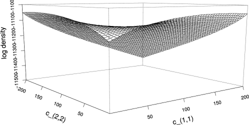
Figure 3: The log-density $\log\bar{\pi}$ as a function of $c_{(1,1)}$ and $c_{(2,2)}$, fixing $c_{(1,2)}=c_{(2,1)}=0$ and for the case $w=2$.

We will use Theorem B.1 to bound $\operatorname{Gap}(T)$. Partition the state space $\mathcal{X}$ of $T$ according to the value of $\mathbf{C}(\mathbf{A})$,

$$D_{\mathbf{c}}\triangleq\bigl{\{}\mathbf{A}\in\mathcal{X}:\mathbf{C}(\mathbf{A})=\mathbf{c}\bigr{\}},\qquad\mathbf{c}\in\bar{\mathcal{X}}.$$ (23)

Define the projection matrix (Appendix B) for $T$ with respect to this partition:

$$\bar{T}(\mathbf{c}_{1},\mathbf{c}_{2}) \triangleq \frac{\sum_{\mathbf{A}:\mathbf{C}(\mathbf{A})=\mathbf{c}_{1}}\pi(\mathbf{A}|\mathbf{S})T(\mathbf{A},D_{\mathbf{c}_{2}})}{\sum_{\mathbf{A}:\mathbf{C}(\mathbf{A})=\mathbf{c}_{1}}\pi(\mathbf{A}|\mathbf{S})}$$

$$= \sum_{\mathbf{A}:\mathbf{C}(\mathbf{A})=\mathbf{c}_{1}}\frac{1}{|D_{\mathbf{c}_{1}}|}T(\mathbf{A},D_{\mathbf{c}_{2}}),\qquad\mathbf{c}_{1},\mathbf{c}_{2}\in\bar{\mathcal{X}}$$

since $\pi(\mathbf{A}|\mathbf{S})$ depends on $\mathbf{A}$ only via $\mathbf{C}(\mathbf{A})$, so that $\pi(\mathbf{A}|\mathbf{S})$ is equal for all $\mathbf{A}\in D_{\mathbf{c}_{1}}$. The matrix $\bar{T}$ is reversible with respect to $\bar{\pi}$ (Appendix B).

It is easier to obtain useful bounds on $\operatorname{Gap}(T)$ indirectly by relating $T$ to $\bar{T}$ and bounding $\operatorname{Gap}(\bar{T})$ than it is to obtain useful bounds on $\operatorname{Gap}(T)$ directly. The same technique is utilized in Madras and Zheng (2003) and Woodard, Schmidler and Huber (2009a). The cardinality of the state space $\mathcal{X}=\{0,1\}^{L/w}$ of $T$ grows exponentially in $L$ for fixed $w$, while the cardinality of the state space $\bar{\mathcal{X}}$ of $\bar{T}$ grows only polynomially in $L$, since [using (20)]

$$|\bar{\mathcal{X}}|\leq(L/w+1)^{2^{w}}.$$ (25)

We obtain an upper bound on $\operatorname{Gap}(\bar{T})$ using conductance (Theorem B.2) and a lower bound on $\operatorname{Gap}(\bar{T})$ using path bounds (Theorem B.4). Bounds obtained using these tools can easily be inaccurate by a factor equal to the cardinality of the space. If we were to obtain these bounds directly for $\operatorname{Gap}(T)$ they would be loose by an exponential factor in $L$, and thus unusable for our purposes.

5.3 Step 1 of proof of Theorem 3.1

Consider the graph associated with the reversible matrix $\bar{T}$, with vertices corresponding to $\mathbf{c}\in\bar{\mathcal{X}}$ and edges corresponding to pairs $\mathbf{c}_{1},\mathbf{c}_{2}\in\bar{\mathcal{X}}$ having $\bar{T}(\mathbf{c}_{1},\mathbf{c}_{2})>0$. For any $\mathbf{c}_{1},\mathbf{c}_{2}\in\bar{\mathcal{X}}$ let $\Gamma_{\mathbf{c}_{1},\mathbf{c}_{2}}$ denote the set of paths between $\mathbf{c}_{1}$ and $\mathbf{c}_{2}$ in the graph that do not have repeated vertices. Also let $\mathbf{c}\in\gamma$ indicate that the state $\mathbf{c}\in\bar{\mathcal{X}}$ is a vertex in the path $\gamma$. Then Theorem 5.1 formalizes step 1 from Section 5.2.

Theorem 5.1

$\operatorname{Gap}(T)$ decreases exponentially in $L$ if and only if

$$d\triangleq\min_{\mathbf{c}_{1},\mathbf{c}_{2}\in\bar{\mathcal{X}}}\max_{\gamma\in\Gamma_{\mathbf{c}_{1},\mathbf{c}_{2}}}\min_{\mathbf{c}\in\gamma}\frac{\bar{\pi}(\mathbf{c}|\mathbf{S})}{\bar{\pi}(\mathbf{c}_{1}|\mathbf{S})\bar{\pi}(\mathbf{c}_{2}|\mathbf{S})}$$ (26)

decreases exponentially in $L$.

The quantity $d$ measures the multimodality of $\bar{\pi}$. Roughly, think of $\mathbf{c}_{1},\mathbf{c}_{2}$ as being local modes of $\bar{\pi}$; if all paths between $\mathbf{c}_{1}$ and $\mathbf{c}_{2}$ contain a state with low probability, then $d$ is small.

Proof of Theorem 5.1 The transition matrix $T$ is nonnegative definite and reversible with respect to $\pi(\mathbf{A}|\mathbf{S})$. Notice that $T^{2}$ is also reversible w.r.t. $\pi(\mathbf{A}|\mathbf{S})$. Using (23), let $T^{2}|_{D_{\mathbf{c}}}$ be the restriction of $T^{2}$ to $D_{\mathbf{c}}$ as defined in Appendix B. Then by Lemma B.1 and Theorem B.1,

$$\operatorname{Gap}(T) \geq \frac{1}{3}\operatorname{Gap}\bigl{(}T^{3}\bigr{)}=\frac{1}{3}\operatorname{Gap}\bigl{(}T^{1/2}T^{2}T^{1/2}\bigr{)}$$

$$\geq \frac{1}{3}\operatorname{Gap}(\bar{T})\min_{\mathbf{c}\in\bar{\mathcal{X}}}\operatorname{Gap}\bigl{(}T^{2}|_{D_{\mathbf{c}}}\bigr{)}.$$

Combining with Proposition 5.1 below, we have that

$$\operatorname{Gap}(T)^{-1}=\mathcal{O}\bigl{(}\operatorname{Gap}(\bar{T})^{-1}\times L^{2w+3}\bigr{)}.$$ (28)

Theorem B.1 also gives the bound $\operatorname{Gap}(T)\leq\operatorname{Gap}(\bar{T}).$ So $\operatorname{Gap}(T)$ is within a polynomial (in $L$) factor of $\operatorname{Gap}(\bar{T})$. Theorem 5.1 then follows from Proposition 5.2 below.

Finally we give several results used in the proof of Theorem 5.1.

Proposition 5.1

We have $[\min_{\mathbf{c}\in\bar{\mathcal{X}}}\operatorname{Gap}(T^{2}|_{D_{\mathbf{c}}})]^{-1}=\mathcal{O}(L^{2w+3})$.

Take any $\mathbf{c}\in\bar{\mathcal{X}}$. For $\mathbf{s}\in\{1,2\}^{w}$ such that $C(\mathbf{S})_{\mathbf{s}}>0$ let $\mathcal{X}_{\mathbf{s}}\triangleq\{\mathbf{z}\in\{0,1\}^{C(\mathbf{S})_{\mathbf{s}}}\dvtx\sum_{i}z_{i}=c_{\mathbf{s}}\}$. Using (19) and (23) the subvector of $\mathbf{A}\in D_{\mathbf{c}}$ defined by $(A_{i}\dvtx\mathbf{S}_{wi-w+1:wi}=\mathbf{s})$ takes values in the space $\mathcal{X}_{\mathbf{s}}$. So there is some bijective map $h$ such that

$$\bigl{\{}h(\mathbf{A})\dvtx\mathbf{A}\in D_{\mathbf{c}}\bigr{\}}=\prod_{\mathbf{s}\in\{1,2\}^{w}\dvtx C(\mathbf{S})_{\mathbf{s}}>0}\mathcal{X}_{\mathbf{s}}.$$ (29)

Define a transition matrix $\tilde{T}$ having state space $\prod_{\mathbf{s}\in\{1,2\}^{w}\dvtx C(\mathbf{S})_{\mathbf{s}}>0}\mathcal{X}_{\mathbf{s}}$ and elements $\tilde{T}(h(\mathbf{A}),h(\mathbf{A}^{\prime}))\triangleq T^{2}|_{D_{\mathbf{c}}}(\mathbf{A},\mathbf{A}^{\prime})$ for all $\mathbf{A},\mathbf{A}^{\prime}\in D_{\mathbf{c}}$. Then we have

$$\operatorname{Gap}(\tilde{T})=\operatorname{Gap}\bigl{(}T^{2}|_{D_{\mathbf{c}}}\bigr{)}.$$ (30)

Using (53) and the fact that $T^{2}$ is reversible w.r.t. $\pi(\mathbf{A}|\mathbf{S})$, $T^{2}|_{D_{\mathbf{c}}}$ is reversible w.r.t. $\pi|_{D_{\mathbf{c}}}(\mathbf{A}|\mathbf{S})$. Since $\pi(\mathbf{A}|\mathbf{S})$ is equal for all $\mathbf{A}\in D_{\mathbf{c}}$, $\pi|_{D_{\mathbf{c}}}(\mathbf{A}|\mathbf{S})$ is uniform on $D_{\mathbf{c}}$, and thus $\tilde{T}$ is also reversible w.r.t. the uniform distribution.

We will compare $\tilde{T}$ to a product chain as defined in Theorem B.3, denoted by $T^{*}$. Define $T^{*}$ to have component chains indexed by $\mathbf{s}\in\{1,2\}^{w}\dvtx C(\mathbf{S})_{\mathbf{s}}>0$. The component chains are denoted by $T_{\mathbf{s}}^{*}$, have state space $\mathcal{X}_{\mathbf{s}}$ and are combined using weights $b_{\mathbf{s}}=\frac{C(\mathbf{S})_{\mathbf{s}}}{L/w}$ to form $T^{*}$. Define $T^{*}_{\mathbf{s}}$ to be the exclusion process with $c_{\mathbf{s}}$ particles on the complete graph of $\{1,\ldots,C(\mathbf{S})_{\mathbf{s}}\}$ [Diaconis and Saloff-Coste (1993)]. This chain is defined informally as follows, where $\mathbf{z}\in\mathcal{X}_{\mathbf{s}}$ is the current state. If $c_{\mathbf{s}}=0$ or $c_{\mathbf{s}}=C(\mathbf{S})_{\mathbf{s}}$, then $\mathcal{X}_{\mathbf{s}}$ has a single state, and the transition matrix $T^{*}_{\mathbf{s}}$ is trivially defined. Otherwise, $T_{\mathbf{s}}^{*}$ chooses an index $j$ uniformly at random from $\{i\in\{1,\ldots,C(\mathbf{S})_{\mathbf{s}}\}\dvtx z_{i}=1\}$. Then it chooses an index $\ell\in\{1,\ldots,C(\mathbf{S})_{\mathbf{s}}\}$ uniformly at random. If $z_{\ell}=0$, then $z_{j}$ is changed to $0$, and $z_{\ell}$ is changed to $1$; otherwise, the state $\mathbf{z}$ does not change. The matrix $T^{*}_{\mathbf{s}}$ is reversible with respect to the distribution $\mu_{\mathbf{s}}$ that is uniform on $\mathcal{X}_{\mathbf{s}}$ [Diaconis and Saloff-Coste (1993)]. So by Theorem B.3, $T^{*}$ is reversible with respect to the uniform distribution on $\prod_{\mathbf{s}\in\{1,2\}^{w}\dvtx C(\mathbf{S})_{\mathbf{s}}>0}\mathcal{X}_{\mathbf{s}}$.

By Theorem 3.1 of Diaconis and Saloff-Coste (1993), for $c_{\mathbf{s}}>0$ we have $\operatorname{Gap}(T_{\mathbf{s}}^{*})\geq 1/{c_{\mathbf{s}}}$, while for $c_{\mathbf{s}}=0$, $\operatorname{Gap}(T_{\mathbf{s}}^{*})=1$. Then Theorem B.3 together with $c_{\mathbf{s}}\leq C(\mathbf{S})_{\mathbf{s}}$ yields

$$\operatorname{Gap}\bigl{(}T^{*}\bigr{)} = \min_{\mathbf{s}\in\{1,2\}^{w}\dvtx C(\mathbf{S})_{\mathbf{s}}>0}b_{\mathbf{s}}\operatorname{Gap}\bigl{(}T_{\mathbf{s}}^{*}\bigr{)}$$

$$\geq \min_{\mathbf{s}\in\{1,2\}^{w}\dvtx C(\mathbf{S})_{\mathbf{s}}>0}\biggl{\{}\frac{C(\mathbf{S})_{\mathbf{s}}}{L/w}\biggl{(}1\wedge\frac{1}{c_{\mathbf{s}}}\biggr{)}\biggr{\}}\geq\frac{w}{L}.$$

By (2.1) and the fact that $\mathbf{C}(\mathbf{A})=\mathbf{C}(\mathbf{A}^{\prime})=\mathbf{c}$ for $\mathbf{A},\mathbf{A}^{\prime}\in D_{\mathbf{c}}$, $T^{2}(\mathbf{A},\mathbf{A}^{\prime})>0$ if and only if $\exists\mathbf{s}\in\{1,2\}^{w}\dvtx C(\mathbf{S})_{\mathbf{s}}>0$ such that $\mathbf{A}^{\prime}$ differs from $\mathbf{A}$ only by swapping two elements of the subvector $(A_{i}\dvtx\mathbf{S}_{wi-w+1:wi}=\mathbf{s})$. Swapping two elements of a vector in $\mathcal{X}_{\mathbf{s}}$ is precisely the move made by the transition matrix $T^{*}_{\mathbf{s}}$. So

$$T^{*}\bigl{(}h(\mathbf{A}),h\bigl{(}\mathbf{A}^{\prime}\bigr{)}\bigr{)}>0\qquad\mbox{iff }T^{2}\bigl{(}\mathbf{A},\mathbf{A}^{\prime}\bigr{)}>0\mbox{ for }\mathbf{A},\mathbf{A}^{\prime}\in D_{\mathbf{c}}\dvtx\mathbf{A}\neq\mathbf{A}^{\prime}.$$ (32)

Using (52),

$$T^{2}|_{D_{\mathbf{c}}}\bigl{(}\mathbf{A},\mathbf{A}^{\prime}\bigr{)}=T^{2}\bigl{(}\mathbf{A},\mathbf{A}^{\prime}\bigr{)}\qquad\forall\mathbf{A},\mathbf{A}^{\prime}\in D_{\mathbf{c}}\dvtx\mathbf{A}\neq\mathbf{A}^{\prime}.$$ (33)

Also, by Lemma 5.1 below,

$$d_{1}\triangleq\Bigl{[}\min_{\mathbf{A},\mathbf{A}^{\prime}\in\mathcal{X}:T^{2}(\mathbf{A},\mathbf{A}^{\prime})>0}T^{2}\bigl{(}\mathbf{A},\mathbf{A}^{\prime}\bigr{)}\Bigr{]}^{-1}=\mathcal{O}\bigl{(}L^{2w+2}\bigr{)}.$$ (34)

Combining with (32) and (33), for any $\mathbf{A},\mathbf{A}^{\prime}\in D_{\mathbf{c}}$ such that $\mathbf{A}\neq\mathbf{A}^{\prime}$ and $T^{*}(h(\mathbf{A}),h(\mathbf{A}^{\prime}))>0$,

$$\tilde{T}\bigl{(}h(\mathbf{A}),h\bigl{(}\mathbf{A}^{\prime}\bigr{)}\bigr{)}=T^{2}\bigl{(}\mathbf{A},\mathbf{A}^{\prime}\bigr{)}\geq d_{1}^{-1}\geq d_{1}^{-1}T^{*}\bigl{(}h(\mathbf{A}),h\bigl{(}\mathbf{A}^{\prime}\bigr{)}\bigr{)}.$$

For $\mathbf{A},\mathbf{A}^{\prime}\in D_{\mathbf{c}}$ such that $\mathbf{A}\neq\mathbf{A}^{\prime}$ and $T^{*}(h(\mathbf{A}),h(\mathbf{A}^{\prime}))=0$ the same inequality holds trivially. So

$$\tilde{T}\bigl{(}h(\mathbf{A}),h\bigl{(}\mathbf{A}^{\prime}\bigr{)}\bigr{)}\geq d_{1}^{-1}T^{*}\bigl{(}h(\mathbf{A}),h\bigl{(}\mathbf{A}^{\prime}\bigr{)}\bigr{)}\qquad\!\!\!\forall h(\mathbf{A})\neq h\bigl{(}\mathbf{A}^{\prime}\bigr{)}\in\!\prod_{\mathbf{s}\in\{1,2\}^{w}\dvtx C(\mathbf{S})_{\mathbf{s}}>0}\!\mathcal{X}_{\mathbf{s}}.$$

By Lemma B.2 and the fact that both $\tilde{T}$ and $T^{*}$ are reversible with respect to the uniform distribution on $\prod_{\mathbf{s}\in\{1,2\}^{w}\dvtx C(\mathbf{S})_{\mathbf{s}}>0}\mathcal{X}_{\mathbf{s}}$, we then have $\operatorname{Gap}(\tilde{T})\geq d_{1}^{-1}\operatorname{Gap}(T^{*})$. Combining with (30) and (5.3),

$$\operatorname{Gap}\bigl{(}T^{2}|_{D_{\mathbf{c}}}\bigr{)}^{-1} = \operatorname{Gap}(\tilde{T})^{-1}\leq d_{1}\operatorname{Gap}\bigl{(}T^{*}\bigr{)}^{-1}$$

$$\leq \frac{d_{1}L}{w}$$

regardless of the value of $\mathbf{c}$. By (34) $d_{1}$ does not depend on $\mathbf{c}$, so$\max_{\mathbf{c}\in\bar{\mathcal{X}}}\operatorname{Gap}(T^{2}|_{D_{\mathbf{c}}})^{-1}=\mathcal{O}(L^{2w+3}).$

Lemma 5.1 was used in the proof of Proposition 5.1.

Lemma 5.1

We have

$$\Bigl{[}\min_{\mathbf{A},\mathbf{A}^{\prime}\in\mathcal{X}:T(\mathbf{A},\mathbf{A}^{\prime})>0}T\bigl{(}\mathbf{A},\mathbf{A}^{\prime}\bigr{)}\Bigr{]}^{-1}=\mathcal{O}\bigl{(}L^{w+1}\bigr{)}.$$

Recall the definition of $\check{\theta}_{k,m}$ from (17). Using (5.1),

$$\pi(A_{i}=1|\mathbf{A}_{[-i]},\mathbf{S})$$

$$\qquad=\Biggl{(}p_{0}\prod_{k=1}^{w}\check{\theta}_{k,S_{wi-w+k}}\Biggr{)}$$

$$\qquad\quad{}\bigg{/}\Biggl{(}p_{0}\prod_{k=1}^{w}\check{\theta}_{k,S_{wi-w+k}}+(1-p_{0})\bigl{(}\Gamma\bigl{(}\mathbf{N}\bigl{(}\mathbf{A}^{c}_{[i,0]}\bigr{)}+\bolds{\beta}_{0}\bigr{)}\Gamma\bigl{(}\bigl{|}\mathbf{N}\bigl{(}\mathbf{A}^{c}_{[i,1]}\bigr{)}\bigl{|}+|\bolds{\beta}_{0}|\bigr{)}\bigr{)}$$

$$\hskip 170.0pt{}/\bigl{(}\Gamma\bigl{(}\mathbf{N}\bigl{(}\mathbf{A}^{c}_{[i,1]}\bigr{)}+\bolds{\beta}_{0}\bigr{)}\Gamma\bigl{(}\bigl{|}\mathbf{N}\bigl{(}\mathbf{A}^{c}_{[i,0]}\bigr{)}\bigl{|}+|\bolds{\beta}_{0}|\bigr{)}\bigr{)}\Biggr{)}$$ (35)

$$\qquad\geq\min\biggl{\{}\frac{1}{2},\Biggl{(}p_{0}\prod_{k=1}^{w}\check{\theta}_{k,S_{wi-w+k}}\Biggr{)}$$

$$\hskip 71.0pt{}\bigg{/}\bigl{(}2(1-p_{0})\bigl{(}\Gamma\bigl{(}\mathbf{N}\bigl{(}\mathbf{A}^{c}_{[i,0]}\bigr{)}+\bolds{\beta}_{0}\bigr{)}\Gamma\bigl{(}\bigl{|}\mathbf{N}\bigl{(}\mathbf{A}^{c}_{[i,1]}\bigr{)}\bigr{|}+|\bolds{\beta}_{0}|\bigr{)}\bigr{)}$$

$$\hskip 124.0pt{}/\bigl{(}\Gamma\bigl{(}\mathbf{N}\bigl{(}\mathbf{A}^{c}_{[i,1]}\bigr{)}+\bolds{\beta}_{0}\bigr{)}\Gamma\bigl{(}\bigl{|}\mathbf{N}\bigl{(}\mathbf{A}^{c}_{[i,0]}\bigr{)}\bigr{|}+|\bolds{\beta}_{0}|\bigr{)}\bigr{)}\bigr{)}\biggr{\}}.$$

Also, by (2.1) and the definitions of $\mathbf{A}_{[i,0]}$ and $\mathbf{A}_{[i,1]}$,

$$N\bigl{(}\mathbf{A}^{c}_{[i,0]}\bigr{)}_{m} = N\bigl{(}\mathbf{A}^{c}_{[i,1]}\bigr{)}_{m}+\sum_{k=1}^{w}\mathbf{1}_{\{\mathbf{S}_{wi-w+k}=m\}},\qquad m\in\{1,2\},$$

$$\bigl{|}\mathbf{N}\bigl{(}\mathbf{A}^{c}_{[i,0]}\bigr{)}\bigr{|} = \bigl{|}\mathbf{N}\bigl{(}\mathbf{A}^{c}_{[i,1]}\bigr{)}\bigr{|}+w.$$

So

$$\frac{\Gamma(\mathbf{N}(\mathbf{A}^{c}_{[i,0]})+\bolds{\beta}_{0})\Gamma(|\mathbf{N}(\mathbf{A}^{c}_{[i,1]})|+|\bolds{\beta}_{0}|)}{\Gamma(\mathbf{N}(\mathbf{A}^{c}_{[i,1]})+\bolds{\beta}_{0})\Gamma(|\mathbf{N}(\mathbf{A}^{c}_{[i,0]})|+|\bolds{\beta}_{0}|)}$$

$$\qquad=\Biggl{(}\prod_{m=1}^{2}\bigl{(}N\bigl{(}\mathbf{A}^{c}_{[i,1]}\bigr{)}_{m}+\beta_{0,m}\bigr{)}\bigl{(}N\bigl{(}\mathbf{A}^{c}_{[i,1]}\bigr{)}_{m}+\beta_{0,m}+1\bigr{)}$$

$$\hskip 56.0pt{}\cdots\bigl{(}N\bigl{(}\mathbf{A}^{c}_{[i,1]}\bigr{)}_{m}+\beta_{0,m}+\sum_{k=1}^{w}\mathbf{1}_{\{S_{wi-w+k}=m\}}-1\bigr{)}\Biggr{)}$$

$$\qquad\quad{}/\bigl{(}\bigl{(}\bigl{|}\mathbf{N}\bigl{(}\mathbf{A}^{c}_{[i,1]}\bigr{)}\bigr{|}+|\bolds{\beta}_{0}|\bigr{)}\bigl{(}\bigl{|}\mathbf{N}\bigl{(}\mathbf{A}^{c}_{[i,1]}\bigr{)}\bigr{|}+|\bolds{\beta}_{0}|+1\bigr{)}$$

$$\hskip 90.0pt{}\cdots\bigl{(}\bigl{|}\mathbf{N}\bigl{(}\mathbf{A}^{c}_{[i,1]}\bigr{)}\bigr{|}+|\bolds{\beta}_{0}|+w-1\bigr{)}\bigr{)}$$

$$\qquad\leq\Biggl{(}\prod_{m=1}^{2}\bigl{(}\bigl{|}\mathbf{N}\bigl{(}\mathbf{A}^{c}_{[i,1]}\bigr{)}\bigr{|}+|\bolds{\beta}_{0}|\bigr{)}\bigl{(}\bigl{|}\mathbf{N}\bigl{(}\mathbf{A}^{c}_{[i,1]}\bigr{)}\bigr{|}+|\bolds{\beta}_{0}|+1\bigr{)}$$

$$\hskip 56.0pt{}\cdots\Biggl{(}\bigl{|}\mathbf{N}\bigl{(}\mathbf{A}^{c}_{[i,1]}\bigr{)}\bigr{|}+|\bolds{\beta}_{0}|+\sum_{k=1}^{w}\mathbf{1}_{\{S_{wi-w+k}=m\}}-1\Biggr{)}\Biggr{)}$$

$$\qquad\quad{}/\bigl{(}\bigl{(}\bigl{|}\mathbf{N}\bigl{(}\mathbf{A}^{c}_{[i,1]}\bigr{)}\bigr{|}+|\bolds{\beta}_{0}|\bigr{)}\bigl{(}\bigl{|}\mathbf{N}\bigl{(}\mathbf{A}^{c}_{[i,1]}\bigr{)}\bigr{|}+|\bolds{\beta}_{0}|+1\bigr{)}$$

$$\hskip 90.0pt{}\cdots\bigl{(}\bigl{|}\mathbf{N}\bigl{(}\mathbf{A}^{c}_{[i,1]}\bigr{)}\bigr{|}+|\bolds{\beta}_{0}|+w-1\bigr{)}\bigr{)}$$

$$\qquad\leq 1.$$

Combining with (17) and (5.3),

$$\pi(A_{i}=1|\mathbf{A}_{[-i]},\mathbf{S})\geq\frac{p_{0}\prod_{k=1}^{w}\check{\theta}_{k,S_{wi-w+k}}}{2}\geq\frac{p_{0}}{2}\prod_{k=1}^{w}\frac{\beta_{k,S_{wi-w+k}}}{L+|\bolds{\beta}_{k}|},$$

which does not depend on $\mathbf{A}$ or $i$. So $[\min_{\mathbf{A},i}\pi(A_{i}=1|\mathbf{A}_{[-i]},\mathbf{S})]^{-1}=\mathcal{O}(L^{w}).$ Analogously, $[\min_{\mathbf{A},i}\pi(A_{i}=0|\mathbf{A}_{[-i]},\mathbf{S})]^{-1}=\mathcal{O}(L^{w}).$ Using (2.1) then yields the desired result.

Proposition 5.2 was used in the proof of Theorem 5.1.

Proposition 5.2

$\operatorname{Gap}(\bar{T})$ is within a polynomial (in $L$) factor of $d$. Specifically, $\operatorname{Gap}(\bar{T})=\mathcal{O}(d\times L^{2^{w}})$ and $\operatorname{Gap}(\bar{T})^{-1}=\mathcal{O}(d^{-1}\times L^{w+1+2^{w+1}+2^{w}})$.

The bounds in Proposition 5.2 only rely on Lemma 5.1 and the fact (25) that $|\bar{\mathcal{X}}|$ grows polynomially in $L$, and could be improved by leveraging additional properties of $\bar{T}$ (at the cost of some technical complexity). However, Proposition 5.2 is sufficient for our purposes.

Proof of Proposition 5.2

Upper bound. Suppress the dependence of $\bar{\pi}(\mathbf{c}|\mathbf{S})$ on $\mathbf{S}$ for simplicity of notation. Let $\mathbf{c}_{1},\mathbf{c}_{2}\in\bar{\mathcal{X}}$ be a pair of states that achieve the minimum in definition (26) of $d$, so that $d=\max_{\gamma\in\Gamma_{\mathbf{c}_{1},\mathbf{c}_{2}}}\min_{\mathbf{c}\in\gamma}\frac{\bar{\pi}(\mathbf{c})}{\bar{\pi}(\mathbf{c}_{1})\bar{\pi}(\mathbf{c}_{2})}.$ For any $\gamma\in\Gamma_{\mathbf{c}_{1},\mathbf{c}_{2}}$, let $\mathbf{c}_{\gamma}\triangleq\operatorname{argmin}_{\mathbf{c}\in\gamma}\frac{\bar{\pi}(\mathbf{c})}{\bar{\pi}(\mathbf{c}_{1})\bar{\pi}(\mathbf{c}_{2})}$ (in the case of a tie choose the state earliest in the path). Defining the set $E=\{\mathbf{c}_{\gamma}:\gamma\in\Gamma_{\mathbf{c}_{1},\mathbf{c}_{2}}\}$, we have

$$d=\max_{\mathbf{c}_{\gamma}\in E}\frac{\bar{\pi}(\mathbf{c}_{\gamma})}{\bar{\pi}(\mathbf{c}_{1})\bar{\pi}(\mathbf{c}_{2})}.$$ (36)

The set $E$ separates $\mathbf{c}_{1}$ and $\mathbf{c}_{2}$ in the sense that there is no path $\gamma\in\Gamma_{\mathbf{c}_{1},\mathbf{c}_{2}}$ that does not include some state in $E$. If $\mathbf{c}_{1}\in E$, then there is some $\gamma\in\Gamma_{\mathbf{c}_{1},\mathbf{c}_{2}}$ for which $\mathbf{c}_{\gamma}=\mathbf{c}_{1}$, and so $d\geq\frac{1}{\bar{\pi}(\mathbf{c}_{2})}\geq 1$. In this case $\operatorname{Gap}(\bar{T})\leq 2d(L/w+1)^{2^{w}}$ holds since $\operatorname{Gap}(\bar{T})\leq 2$.

Now consider the case $\mathbf{c}_{1}\notin E$. Let $B$ be the set of states $\mathbf{c}\in\bar{\mathcal{X}}$ that are not reachable from $\mathbf{c}_{1}$ without going through $E$,

$$B\triangleq\bigl{\{}\mathbf{c}\in\bar{\mathcal{X}}\dvtx\forall\gamma\in\Gamma_{\mathbf{c}_{1},\mathbf{c}}\mbox{ there is some }\mathbf{c}^{\prime}\in\gamma\mbox{ s.t. }\mathbf{c}^{\prime}\in E\bigr{\}}.$$

We have that $\mathbf{c}_{2}\in B$, and $\mathbf{c}_{1}\in B^{c}$ since $\mathbf{c}_{1}\notin E$. Also, the only states $\mathbf{c}\in B$ for which $\bar{T}(\mathbf{c},B^{c})>0$ satisfy $\mathbf{c}\in E$, which can be seen as follows. Otherwise, $\exists\mathbf{c}\in B\setminus E$ and $\mathbf{c}_{3}\in B^{c}$ for which $\bar{T}(\mathbf{c},\mathbf{c}_{3})>0$. Since $\mathbf{c}_{3}\in B^{c}$, there is a path $\gamma\in\Gamma_{\mathbf{c}_{1},\mathbf{c}_{3}}$ that does not go through $E$. But since $\bar{T}(\mathbf{c}_{3},\mathbf{c})>0$ ($\bar{T}$ is reversible), there is also a path $\gamma\in\Gamma_{\mathbf{c}_{1},\mathbf{c}}$ that does not go through $E$, which is a contradiction.

Using these facts, (25) and (36), the conductance of $B$ (Theorem B.2) is

$$\Phi_{\bar{T}}(B) = \frac{\sum_{\mathbf{c}\in B}\bar{\pi}(\mathbf{c})\bar{T}(\mathbf{c},B^{c})}{\bar{\pi}(B)\bar{\pi}(B^{c})}\leq\frac{\sum_{\mathbf{c}\in E}\bar{\pi}(\mathbf{c})\bar{T}(\mathbf{c},B^{c})}{\bar{\pi}(B)\bar{\pi}(B^{c})}$$

$$\leq \frac{\sum_{\mathbf{c}\in E}\bar{\pi}(\mathbf{c})}{\bar{\pi}(B)\bar{\pi}(B^{c})}\leq\frac{\sum_{\mathbf{c}\in E}\bar{\pi}(\mathbf{c})}{\bar{\pi}(\mathbf{c}_{1})\bar{\pi}(\mathbf{c}_{2})}$$

$$\leq |E|\max_{\mathbf{c}\in E}\frac{\bar{\pi}(\mathbf{c})}{\bar{\pi}(\mathbf{c}_{1})\bar{\pi}(\mathbf{c}_{2})}=|E|d\leq|\bar{\mathcal{X}}|d\leq d(L/w+1)^{2^{w}}.$$

Using Theorem B.2, $\operatorname{Gap}(\bar{T})\leq 2\Phi_{\bar{T}}(B)\leq 2d(L/w+1)^{2^{w}}$ as claimed.

Lower bound. Recall that the transition matrix $\bar{T}$ has state space $\bar{\mathcal{X}}$ and is reversible with respect to $\bar{\pi}$. Using (23)–(5.2), for $\mathbf{c},\mathbf{c}^{\prime}\in\bar{\mathcal{X}}$ such that $\sum_{\mathbf{s}}|c_{\mathbf{s}}-c^{\prime}_{\mathbf{s}}|\leq 1$, $\bar{T}(\mathbf{c},\mathbf{c}^{\prime})>0$ and otherwise $\bar{T}(\mathbf{c},\mathbf{c}^{\prime})=0$. Also

$$\bar{T}\bigl{(}\mathbf{c},\mathbf{c}^{\prime}\bigr{)}\geq\min_{\mathbf{A}\in D_{\mathbf{c}}}T(\mathbf{A},D_{\mathbf{c}^{\prime}})\geq\min_{\mathbf{A}\in D_{\mathbf{c}}}\max_{\mathbf{A}^{\prime}\in D_{\mathbf{c}^{\prime}}}T\bigl{(}\mathbf{A},\mathbf{A}^{\prime}\bigr{)}\qquad\forall\mathbf{c},\mathbf{c}^{\prime}\in\bar{\mathcal{X}}.$$ (37)

If $\bar{T}(\mathbf{c},\mathbf{c}^{\prime})>0$, then for every $\mathbf{A}\in D_{\mathbf{c}}$ there is some $\mathbf{A}^{\prime}\in D_{\mathbf{c}^{\prime}}$ with $T(\mathbf{A},\mathbf{A}^{\prime})>0$. By Lemma 5.1 and (37),

$$\Bigl{[}\min_{\mathbf{c},\mathbf{c}^{\prime}\in\bar{\mathcal{X}}\dvtx\bar{T}(\mathbf{c},\mathbf{c}^{\prime})>0}\bar{T}\bigl{(}\mathbf{c},\mathbf{c}^{\prime}\bigr{)}\Bigr{]}^{-1}=\mathcal{O}\bigl{(}L^{w+1}\bigr{)}.$$ (38)

We will use Theorem B.4 to obtain a bound for $\operatorname{Gap}(\bar{T})$; let $\mathcal{E}$ be the set of edges in the graph of $\bar{T}$. For $(z,v)\in\mathcal{E}$ and $\gamma$ a path in the graph, let $(z,v)\in\gamma$ indicate that the edge $(z,v)$ is in the path $\gamma$ (as distinct from $z\in\gamma$ which indicates that the vertex $z$ is in $\gamma$). To apply Theorem B.4 we need to define a path $\gamma_{x,y}$ for every pair of states $x,y\in\bar{\mathcal{X}}$. Suppressing the dependence of $\bar{\pi}$ on $\mathbf{S}$, choose $\gamma_{x,y}$ to be any path that maximizes $\min_{(z,v)\in\gamma}\frac{\bar{\pi}(z)}{\bar{\pi}(x)\bar{\pi}(y)}$. Letting $|\{\ldots\}|$ denote the cardinality of a set, the path constant $\rho$ defined in Theorem B.4 satisfies

$$\rho = \max_{(z,v)\in\mathcal{E}}\frac{1}{\bar{\pi}(z)\bar{T}(z,v)}\sum_{\gamma_{x,y}\ni(z,v)}\bar{\pi}(x)\bar{\pi}(y)\operatorname{len}(\gamma_{x,y})$$

$$\leq \frac{1}{\min_{(z,v)\in\mathcal{E}}\bar{T}(z,v)}\biggl{[}\max_{(z,v)\in\mathcal{E}}\frac{1}{\bar{\pi}(z)}\sum_{\gamma_{x,y}\ni(z,v)}\bar{\pi}(x)\bar{\pi}(y)\biggr{]}\max_{x,y}\operatorname{len}(\gamma_{x,y})$$

$$\leq \frac{1}{\min_{(z,v)\in\mathcal{E}}\bar{T}(z,v)}\Bigl{[}\max_{(z,v)\in\mathcal{E}}\bigl{|}\bigl{\{}\gamma_{x,y}\ni(z,v)\bigr{\}}\bigr{|}\Bigr{]}$$

$${}\times\biggl{[}\max_{(z,v)\in\mathcal{E}}\max_{\gamma_{x,y}\ni(z,v)}\frac{\bar{\pi}(x)\bar{\pi}(y)}{\bar{\pi}(z)}\biggr{]}\max_{x,y}\operatorname{len}(\gamma_{x,y})$$

$$= \frac{1}{\min_{(z,v)\in\mathcal{E}}\bar{T}(z,v)}\Bigl{[}\max_{(z,v)\in\mathcal{E}}\bigl{|}\bigl{\{}\gamma_{x,y}\ni(z,v)\bigr{\}}\bigr{|}\Bigr{]}$$

$${}\times\biggl{[}\min_{x,y\in\bar{\mathcal{X}}}\min_{(z,v)\in\gamma_{x,y}}\frac{\bar{\pi}(z)}{\bar{\pi}(x)\bar{\pi}(y)}\biggr{]}^{-1}\max_{x,y}\operatorname{len}(\gamma_{x,y})$$

$$= \frac{1}{\min_{(z,v)\in\mathcal{E}}\bar{T}(z,v)}\Bigl{[}\max_{(z,v)\in\mathcal{E}}\bigl{|}\bigl{\{}\gamma_{x,y}\ni(z,v)\bigr{\}}\bigr{|}\Bigr{]}$$

$${}\times\biggl{[}\min_{x,y\in\bar{\mathcal{X}}}\max_{\gamma\in\Gamma_{x,y}}\min_{(z,v)\in\gamma}\frac{\bar{\pi}(z)}{\bar{\pi}(x)\bar{\pi}(y)}\biggr{]}^{-1}\max_{x,y}\operatorname{len}(\gamma_{x,y})$$

$$\leq \frac{1}{\min_{(z,v)\in\mathcal{E}}\bar{T}(z,v)}\Bigl{[}\max_{(z,v)\in\mathcal{E}}\bigl{|}\bigl{\{}\gamma_{x,y}\ni(z,v)\bigr{\}}\bigr{|}\Bigr{]}$$

$${}\times\biggl{[}\min_{x,y\in\bar{\mathcal{X}}}\max_{\gamma\in\Gamma_{x,y}}\min_{z\in\gamma}\frac{\bar{\pi}(z)}{\bar{\pi}(x)\bar{\pi}(y)}\biggr{]}^{-1}\max_{x,y}\operatorname{len}(\gamma_{x,y}).$$

From (25) $|\bar{\mathcal{X}}|=\mathcal{O}(L^{2^{w}})$, so the maximum length of paths is$\max_{x,y}\operatorname{len}(\gamma_{x,y})=\mathcal{O}(L^{2^{w}})$, and the total number of paths is no more than $|\bar{\mathcal{X}}|^{2}=\mathcal{O}(L^{2^{w+1}})$. By Theorem B.4 and (38), $\operatorname{Gap}(\bar{T})^{-1}\leq\rho=\break\mathcal{O}(d^{-1}L^{w+1+2^{w+1}+2^{w}}).$

5.4 Step 2 of proof of Theorem 3.1

Recalling that $M=2$, there are $w+1$ free parameters $\theta_{k,1}\in[0,1]$ for $k\in\{0,\ldots,w\}$, so we write

$$\bolds{\theta}_{0:w}\in[0,1]^{w+1}.$$ (39)

Theorem 5.2 formalizes step 2, using Theorem A.1.

Theorem 5.2

Under Assumption 3.1, if $E\log f(\mathbf{s}|\bolds{\theta}_{0:w})$ is multimodal, then there exist $\varepsilon>0$ and two sets $B_{1},B_{2}\subset[0,1]^{w+1}$ separated by Euclidean distance $\varepsilon$ such that

$$\frac{\pi(\bolds{\theta}_{0:w}\notin B_{1}\cup B_{2}|\mathbf{S})}{\pi(\bolds{\theta}_{0:w}\in B_{1}|\mathbf{S})}\quad\mbox{and}\quad\frac{\pi(\bolds{\theta}_{0:w}\notin B_{1}\cup B_{2}|\mathbf{S})}{\pi(\bolds{\theta}_{0:w}\in B_{2}|\mathbf{S})}$$ (40)

decrease exponentially in $L$, almost surely.

The inference model assumes $\mathbf{S}_{wi-w+1:wi}\stackrel{{\scriptstyle\mathrm{i.i.d.}}}{{\sim}}f(\mathbf{s}|\bolds{\theta}_{0:w})$ for $i\in\{1,\ldots,L/w\}$. By Assumption 3.1, the generative model assumes$\mathbf{S}_{wi-w+1:wi}\stackrel{{\scriptstyle\mathrm{i.i.d.}}}{{\sim}}g(\mathbf{s})$, fitting into the framework of Theorem A.1. Using the notation of that theorem, consider the case where $\eta(\bolds{\theta}_{0:w})=E\log f(\mathbf{s}|\bolds{\theta}_{0:w})$ is multimodal. Then there are $\bolds{\theta}_{0:w}^{(j)}\in[0,1]^{w+1}$ and $F_{j}\subset[0,1]^{w+1}$ for $j\in\{1,2\}$ such that $\bolds{\theta}_{0:w}^{(j)}\in F_{j}$ and (10) holds. Let $\phi_{j}\triangleq\sup_{\partial F_{j}}\eta(\bolds{\theta}_{0:w})<\eta(\bolds{\theta}_{0:w}^{(j)})$ for $j\in\{1,2\}$, and take any $\xi$ for which

$$\xi\in\Bigl{(}\min_{j\in\{1,2\}}\phi_{j},\min_{j\in\{1,2\}}\eta\bigl{(}\bolds{\theta}_{0:w}^{(j)}\bigr{)}\Bigr{)}.$$ (41)

So $\xi>\phi_{j}$ for some $j\in\{1,2\}$; assume WLOG that $\xi>\phi_{1}$.

Define the sets

$$V \triangleq \bigl{\{}\bolds{\theta}_{0:w}\in[0,1]^{w+1}:\eta(\bolds{\theta}_{0:w})\geq\xi\bigr{\}},$$

$$\tilde{B}_{1} \triangleq F_{1}\cap V,\qquad\tilde{B}_{2}\triangleq V\setminus F_{1}.$$

By (41), $\eta(\bolds{\theta}_{0:w}^{(1)})>\xi$ and $\bolds{\theta}_{0:w}^{(1)}\in\tilde{B}_{1}$. Also using (10), $\eta(\bolds{\theta}_{0:w}^{(2)})>\xi$ and $\bolds{\theta}^{(2)}_{0:w}\in F_{2}\cap V\subset\tilde{B}_{2}$, so

$$V=\tilde{B}_{1}\cup\tilde{B}_{2}\quad\mbox{and}\quad\sup_{\bolds{\theta}_{0:w}\in\tilde{B}_{j}}\eta(\bolds{\theta}_{0:w})>\xi,\qquad j\in\{1,2\}.$$ (43)

If $\nexists\varepsilon>0$ such that $\tilde{B}_{1}$ and $\tilde{B}_{2}$ are separated by distance $\varepsilon$, then (since $[0,1]^{w+1}$ is compact) $\operatorname{cl}(\tilde{B}_{1})\cap\operatorname{cl}(\tilde{B}_{2})\neq\varnothing$. By (5.4) $\tilde{B}_{1}\subset F_{1}$ and $\tilde{B}_{2}\subset[0,1]^{w+1}\setminus F_{1}$ so $\operatorname{cl}(\tilde{B}_{1})\cap\operatorname{cl}(\tilde{B}_{2})\subset\partial F_{1}$. This is a contradiction since, due to (5.4)–(43) and the continuity of $\eta$,

$$\inf_{\operatorname{cl}(\tilde{B}_{1})\cap\operatorname{cl}(\tilde{B}_{2})}\eta\geq\inf_{\operatorname{cl}(\tilde{B}_{1})\cup\operatorname{cl}(\tilde{B}_{2})}\eta=\inf_{\tilde{B}_{1}\cup\tilde{B}_{2}}\eta\geq\xi>\phi_{1}=\sup_{\partial F_{1}}\eta.$$

So $\exists\varepsilon>0$ such that $\tilde{B}_{1}$ and $\tilde{B}_{2}$ are separated by distance $\varepsilon$.

In order to satisfy assumption (2) of Theorem A.1 we remove points from the space $[0,1]^{w+1}$ of $\bolds{\theta}_{0:w}$ for which $\exists\mathbf{s}\in\{1,2\}^{w}\dvtx f(\mathbf{s}|\bolds{\theta}_{0:w})=0$. This results in the space

$$\Lambda=\bigl{(}(0,1)\times[0,1]^{w}\bigr{)}\cup\bigl{(}[0,1]\times(0,1)^{w}\bigr{)}.$$ (44)

The fact that $f(\mathbf{s}|\bolds{\theta}_{0:w})>0$ for all $\mathbf{s}$ and all $\bolds{\theta}_{0:w}\in\Lambda$ is a consequence of (8): if $\theta_{0,1}\in(0,1)$, then $f(\mathbf{s}|\bolds{\theta}_{0:w})>0$ for all $\mathbf{s}$, and the same holds when $\theta_{k,1}\in(0,1)$ for all $k\in\{1,\ldots,w\}$.

Taking

$$B_{j}\triangleq\tilde{B}_{j}\cap\Lambda,\qquad j\in\{1,2\}$$ (45)

$B_{1}$ and $B_{2}$ are separated by distance $\varepsilon$. Due to (10), $\bolds{\theta}_{0:w}^{(j)}$ is not a limit point of $[0,1]^{w+1}\setminus F_{j}$ for $j\in\{1,2\}$. Using (44) there are points $\bolds{\theta}_{0:w}\in\Lambda$ arbitrarily close to $\bolds{\theta}_{0:w}^{(j)}\in[0,1]^{w+1}$. From (41) and the continuity of $\eta$, all such points $\bolds{\theta}_{0:w}$ close enough to $\bolds{\theta}_{0:w}^{(j)}$ have $\bolds{\theta}_{0:w}\in F_{j}\cap\Lambda$ and $\eta(\bolds{\theta}_{0:w})>\xi$. Using (10), (5.4) and (45) these points are in $B_{j}$, so

$$\sup_{\bolds{\theta}_{0:w}\in B_{j}}\eta(\bolds{\theta}_{0:w})>\xi,\qquad j\in\{1,2\}.$$ (46)

Let $\operatorname{Int}(\cdot)$ denote set interior with respect to the space $\Lambda$. We claim that

$$\bigl{\{}\bolds{\theta}_{0:w}\in\Lambda:\eta(\bolds{\theta}_{0:w})>\xi\bigr{\}}\subset\operatorname{Int}(B_{1})\cup\operatorname{Int}(B_{2}),$$ (47)

which can be seen as follows. Take any $\bolds{\theta}_{0:w}\in\Lambda$ such that $\eta(\bolds{\theta}_{0:w})>\xi$. By (5.4), (43), (45) and since $\eta$ is continuous, $\bolds{\theta}_{0:w}\in\operatorname{Int}(B_{1}\cup B_{2})$. Because $B_{1}$ and $B_{2}$ are separated by distance $\varepsilon>0$, $\bolds{\theta}_{0:w}\in\operatorname{Int}(B_{1})\cup\operatorname{Int}(B_{2})$.

Define the alternative parameter spaces $\Lambda_{1}\triangleq\Lambda\setminus\operatorname{Int}(B_{2})$ and $\Lambda_{2}\triangleq\Lambda\setminus\operatorname{Int}(B_{1})$. By (46), $\sup_{\Lambda_{j}}\eta>\xi$ for $j\in\{1,2\}$. So $\delta_{j}\triangleq\frac{\sup_{\Lambda_{j}}\eta-\xi}{2}>0$ for $j\in\{1,2\}$. Combining (47) with the fact that $\sup_{\Lambda_{j}}\eta-\delta_{j}>\xi$,

$$U^{j}_{\delta_{j}}\triangleq\Bigl{\{}\bolds{\theta}_{0:w}\in\Lambda_{j}\dvtx\eta(\bolds{\theta}_{0:w})\geq\sup_{\Lambda_{j}}\eta-\delta_{j}\Bigr{\}}\subset\operatorname{Int}(B_{j})\subset B_{j},$$

(48)

$$\eqntext{j\in\{1,2\}.}$$ (49)

By (5.4),

$$\qquad\Lambda\setminus(B_{1}\cup B_{2})\subset\Lambda\setminus\bigl{(}B_{1}\cup\operatorname{Int}(B_{2})\bigr{)}\subset\Lambda\setminus\bigl{(}U^{1}_{\delta_{1}}\cup\operatorname{Int}(B_{2})\bigr{)}=\Lambda_{1}\setminus U^{1}_{\delta_{1}}.$$ (50)

Analogously, $\Lambda\setminus(B_{1}\cup B_{2})\subset\Lambda_{2}\setminus U^{2}_{\delta_{2}}$.

The regularity conditions of Theorem A.1 are verified in the supplementary material [Woodard and Rosenthal (2013)] for each of the parameter spaces $\Lambda_{1}$ and $\Lambda_{2}$. We apply that theorem for each of $j\in\{1,2\}$, with parameter space $\Lambda_{j}$, using $\delta=\delta_{j}$ and taking $n=L/w$. This yields

$$\limsup_{n\rightarrow\infty}\biggl{(}\frac{P_{n}(\Lambda_{j}\setminus U^{j}_{\delta_{j}})}{P_{n}(U^{j}_{\delta_{j}})}\biggr{)}^{1/n}\leq e^{-\delta_{j}}\qquad\mbox{a.s. }j\in\{1,2\}.$$

Combining with (5.4)–(50) and the fact that $[0,1]^{w+1}\setminus\Lambda$ has probability zero under $\pi(\bolds{\theta}_{0:w}|\mathbf{S})$, for $j\in\{1,2\}$

$$\limsup_{L\rightarrow\infty}\biggl{(}\frac{\pi(\bolds{\theta}_{0:w}\in[0,1]^{w+1}\setminus(B_{1}\cup B_{2})|\mathbf{S})}{\pi(\bolds{\theta}_{0:w}\in B_{j}|\mathbf{S})}\biggr{)}^{{1}/{(L/w)}}$$

$$\qquad=\limsup_{L\rightarrow\infty}\biggl{(}\frac{\pi(\bolds{\theta}_{0:w}\in\Lambda\setminus(B_{1}\cup B_{2})|\mathbf{S})}{\pi(\bolds{\theta}_{0:w}\in B_{j}|\mathbf{S})}\biggr{)}^{{1}/{(L/w)}}$$

$$\qquad\leq\limsup_{L\rightarrow\infty}\biggl{(}\frac{\pi(\bolds{\theta}_{0:w}\in\Lambda_{j}\setminus U_{\delta_{j}}^{j}|\mathbf{S})}{\pi(\bolds{\theta}_{0:w}\in U_{\delta_{j}}^{j}|\mathbf{S})}\biggr{)}^{{1}/{(L/w)}}$$

$$\qquad=\limsup_{n\rightarrow\infty}\biggl{(}\frac{P_{n}(\Lambda_{j}\setminus U^{j}_{\delta_{j}})}{P_{n}(U^{j}_{\delta_{j}})}\biggr{)}^{1/n}\leq e^{-\delta_{j}}$$

almost surely.

5.5 Step 3 of proof of Theorem 3.1

Finally we formalize step 3.

Theorem 5.3

If there exist $\varepsilon>0$ and two sets $B_{1},B_{2}\subset[0,1]^{w+1}$ separated by Euclidean distance $\varepsilon$ such that the ratios in (40) decrease exponentially in $L$, then the quantity $d$ in (26) decreases exponentially in $L$.

Theorem 5.3 is proven in the supplementary material [Woodard and Rosenthal (2013)]. Theorems 5.1–5.3 together imply Theorem 3.1.

6 Conclusions

The Gibbs sampling method is a popular approach to finding gene regulatory binding motifs, but its poor convergence in practice means that it can only be used to generate candidate motifs that must be ranked using a secondary criterion. If one could efficiently obtain samples from the posterior distribution, these samples could be used to directly find the “best,” that is, most probable, motifs, obviating the need for secondary analysis. We have obtained theoretical and empirical results showing that the convergence of the Gibbs sampler is even worse than previously realized. Our results reinforce the need to convey the limitations of any estimates obtained using the Gibbs sampler, and the need to develop more efficient Markov chain methods for motif discovery.

Although our main result (Theorem 3.1) is phrased in terms of a specific model, the methods used to prove this result are very widely applicable to situations with i.i.d. data, where the data are not necessarily generated according to the model, and where the function $E\log f(X|\theta)$ is multimodal. The extent to which slow mixing holds in other contexts will be determined by how generally this multimodality condition holds, so we are currently investigating this condition in detail.

Appendix A Bayesian asymptotics

We quote a result from Berk (1966) on Bayesian asymptotics for i.i.d. observations. Let $f(x|\theta)$ be the density (with respect to some $\sigma$-finite measure on a space $\mathcal{Y}$) of each observation $X_{i}$ under the inference model, parameterized by $\theta\in\Lambda$ where $\Lambda$ is a Borel subset of a complete separable metric space. Let the true distribution of the observations be denoted by $G$. Define:[(1)]

The “carrier” of a distribution $P$: the smallest relatively closed set having probability one under $P$.

$P_{n}$: the posterior distribution of $\theta$ with $n$ observations, with respect to a prior $P$ having carrier $\Lambda$.

$\eta(\theta)\triangleq E\log f(X|\theta)$ where the expectation is taken with respect to $X\sim G$.

$\eta^{*}\triangleq\sup\{\eta(\theta)\dvtx\theta\in\Lambda\}$.

$U_{\delta}\triangleq\{\theta\in\Lambda:\eta(\theta)\geq\eta^{*}-\delta\}$ for $\delta\geq 0$. Assume that:

[(1)]

$f(x|\theta)$ is measurable jointly in $x$ and $\theta$; for $G$-almost every $x$, $f(x|\theta)$ is continuous in $\theta$.

For all $\theta\in\Lambda$, $G\{x\dvtx f(x|\theta)>0\}=1$.

For any compact $F\subset\Lambda$, $E\sup_{\theta\in F}|\log f(X|\theta)|<\infty$.

$\eta(\theta)$ is continuous.

For any real number $r$ there is a co-compact set $D\subset\Lambda$ ($D^{c}=\Lambda\setminus D$ is compact) and a cover $D_{1},\ldots,D_{K}$ of $D$ such that

$$E\sup_{\theta\in D_{k}}\log f(X|\theta)\leq r,\qquad k\in\{1,\ldots,K\}.$$ (51)

With these assumptions, we have Theorem A.1.

Theorem A.1 ([Berk (1966)])

For $G$-almost every sequence of observations $\{x_{i}\dvtx i\in\mathbb{N}\}$ and any $\delta>0$,

$$\limsup_{n\rightarrow\infty}\biggl{(}\frac{P_{n}(\Lambda\setminus U_{\delta})}{P_{n}(U_{\delta})}\biggr{)}^{1/n}\leq e^{-\delta}.$$

Theorem A.1 is a sub-result given in the proof of Berk’s main theorem. It says that the posterior probability of $U_{\delta}^{c}$ decreases exponentially in $n$. Here we have stated the result slightly more generally than Berk (1966) in the sense that we replace his assumption (iii) with the only two relevant consequences of that assumption: our assumptions (3)–(4). Also, in our assumption (5) we have allowed a cover of $D$, whereas Berk’s assumption (iv) takes $K=1$. The extension to the case of general $K$ is immediate from his proof.

Appendix B Tools for bounding spectral gaps

Let $P$ and $Q$ be transition kernels that are reversible with respect to distributions $\mu_{P}$ and $\mu_{Q}$ on a (general) state space $\mathcal{X}$ with countably-generated $\sigma$-algebra. Let $P|_{B}$ for $B\subset\mathcal{X}$ indicate the restriction of $P$ to $B$, which is defined to have state space $B$ and transition probabilities identical to $P$ except that any move to $B^{c}$ is rejected,

$$P|_{B}(x,D)=P(x,D)+\mathbf{1}_{\{x\in D\}}P\bigl{(}x,B^{c}\bigr{)},\qquad x\in B,D\subset B.$$ (52)

Also let $\mu_{P}|_{B}$ be the restriction of $\mu_{P}$ to $B$, that is,

$$\mu_{P}|_{B}(dx)\triangleq\mu_{P}(dx)/\mu_{P}(B),\qquad x\in B.$$ (53)

Then $P|_{B}$ is reversible w.r.t. $\mu_{P}|_{B}$.

For a partition $\{B_{j}\}_{j=1}^{J}$ of $\mathcal{X}$, let $\bar{P}$ be the projection matrix of $P$ with respect to $\{B_{j}\}_{j=1}^{J}$, defined to have state space $\{1,\ldots,J\}$ and $i,j$ element equal to the probability that $P$ transitions to $B_{j}$, given that the current state is in $B_{i}$. That is,

$$\bar{P}(i,j)\triangleq\int\mu_{P}|_{B_{i}}(dx)P(x,B_{j}),\qquad i,j\in\{1,\ldots,J\}.$$

The matrix $\bar{P}$ is reversible w.r.t. $\bar{\mu}$, where $\bar{\mu}(j)\triangleq\mu_{P}(B_{j})$.

Lemma B.1 ([Madras and Zheng (2003)])

For any $N\in\mathbb{N}$ we have$\operatorname{Gap}(P)\geq\frac{1}{N}\operatorname{Gap}(P^{N})$.

Although Madras and Zheng (2003) state this result for finite state spaces, their proof also holds for general state spaces.

Theorem B.1 ([Madras and Randall (2002)])

Let $\mu_{P}=\mu_{Q}$, and let $\{B_{j}\}_{j=1}^{J}$ be any partition of $\mathcal{X}$. Assume that $P$ is nonnegative definite and let $P^{1/2}$ be its nonnegative square root. Then

$$\operatorname{Gap}\bigl{(}P^{1/2}QP^{1/2}\bigr{)} \geq \operatorname{Gap}(\bar{P})\min_{j}\operatorname{Gap}(Q|_{B_{j}}),$$

$$\operatorname{Gap}(P) \leq \operatorname{Gap}(\bar{P}),$$

where $\bar{P}$ is the projection matrix of $P$ with respect to $\{B_{j}\}_{j=1}^{J}$.

Theorem B.2 ([E.g., Sinclair (1992)])

For $\mathcal{X}$ finite define

$$\Phi_{P}\triangleq\min_{B\subset\mathcal{X}:0<\mu_{P}(B)<1}\Phi_{P}(B),\qquad\Phi_{P}(B)\triangleq\frac{\sum_{x\in B}\mu_{P}(x)P(x,B^{c})}{\mu_{P}(B)\mu_{P}(B^{c})}.$$

Here $\Phi_{P}$ is called the “conductance,” and $\Phi_{P}(B)$ is referred to as the conductance of the set $B$. Then $\operatorname{Gap}(P)\leq 2\Phi_{P}$.

Theorem B.3 ([Diaconis and Saloff-Coste (1996)])

Take any $N\in\mathbb{N}$, and let $P_{k}$, $k=0,\ldots,N$, be $\mu_{k}$-reversible transition kernels on state spaces $\mathcal{X}_{k}$. Let $P$ be the transition kernel with state $\mathbf{x}=(x_{0},\ldots,x_{N})$ in the space $\mathcal{X}=\prod_{k}\mathcal{X}_{k}$, given by

$$P(\mathbf{x},d\mathbf{y})=\sum_{k=0}^{N}b_{k}P_{k}(x_{k},dy_{k})\delta_{\mathbf{x}_{[-k]}}(\mathbf{y}_{[-k]})\,d\mathbf{y}_{[-k]},\qquad\mathbf{x},\mathbf{y}\in\mathcal{X}$$

for some set of $b_{k}>0$ such that $\sum_{k}b_{k}=1$, where $\delta$ is Dirac’s delta function, and where $\mathbf{x}_{[-k]}$ indicates the vector $\mathbf{x}$ excluding $x_{k}$. $P$ is called a product chain with “component” chains $P_{k}$. It is reversible with respect to $\mu_{P}(dx)=\prod_{k}\mu_{k}(dx_{k})$, and

$$\operatorname{Gap}(P)=\min_{k=0,\ldots,N}b_{k}\operatorname{Gap}(P_{k}).$$

Lemma 3.2 of Diaconis and Saloff-Coste (1996) states Theorem B.3 for finite state spaces; however, the proof holds in the general case.

Lemma B.2

Take finite $\mathcal{X}$ and $\mu_{P}=\mu_{Q}$. If $\exists b>0$ such that $bQ(x,y)\leq P(x,y)$ for every $x,y\in\mathcal{X}$ such that $x\neq y$, then $b\operatorname{Gap}(Q)\leq\operatorname{Gap}(P)$.

The proof is nearly identical to that of Lemma 5.1 in Woodard, Schmidler and Huber (2009a).

Lemma B.2 is closely related to Peskun ordering results; cf. Peskun (1973), Tierney (1998), Mira (2001).

Theorem B.4 ([Sinclair (1992), Diaconis and Stroock (1991)])

For $\mathcal{X}$ finite, define a simple path $\gamma_{x,y}$ between every ordered pair $x,y\in\mathcal{X}$ in the graph of the Markov chain with transition matrix $P$. A simple path is a sequence of connected edges with no repeated vertices. Define the quantity

$$\rho\triangleq\max_{(z,v)\in\mathcal{E}}\frac{1}{\mu_{P}(z)P(z,v)}\sum_{\gamma_{x,y}\ni(z,v)}\mu_{P}(x)\mu_{P}(y)\operatorname{len}(\gamma_{x,y}),$$

where $\mathcal{E}$ is the set of edges, where $\gamma_{x,y}\ni(z,v)$ is a path using the edge $(z,v)$, and where $\operatorname{len}(\gamma_{x,y})$ is the number of edges in $\gamma_{x,y}$. Then $\operatorname{Gap}(P)\geq\rho^{-1}$.

References

- Andrieu, Doucet and Holenstein (2010) {barticle}[mr] \bauthor\bsnmAndrieu, \bfnmChristophe\binitsC., \bauthor\bsnmDoucet, \bfnmArnaud\binitsA. and \bauthor\bsnmHolenstein, \bfnmRoman\binitsR. (\byear2010). \btitleParticle Markov chain Monte Carlo methods (with discussion). \bjournalJ. R. Stat. Soc. Ser. B Stat. Methodol. \bvolume72 \bpages269–342. \biddoi=10.1111/j.1467-9868.2009.00736.x, issn=1369-7412, mr=2758115 \bptnotecheck related\bptokimsref \endbibitem
- Belloni and Chernozhukov (2009) {barticle}[mr] \bauthor\bsnmBelloni, \bfnmAlexandre\binitsA. and \bauthor\bsnmChernozhukov, \bfnmVictor\binitsV. (\byear2009). \btitleOn the computational complexity of MCMC-based estimators in large samples. \bjournalAnn. Statist. \bvolume37 \bpages2011–2055. \biddoi=10.1214/08-AOS634, issn=0090-5364, mr=2533478 \bptokimsref \endbibitem
- Berk (1966) {barticle}[mr] \bauthor\bsnmBerk, \bfnmRobert H.\binitsR. H. (\byear1966). \btitleLimiting behavior of posterior distributions when the model is incorrect. \bjournalAnn. Math. Statist. \bvolume37 \bpages51–58. \bptokimsref \endbibitem
- Bhatnagar and Randall (2004) {binproceedings}[mr] \bauthor\bsnmBhatnagar, \bfnmNayantara\binitsN. and \bauthor\bsnmRandall, \bfnmDana\binitsD. (\byear2004). \btitleTorpid mixing of simulated tempering on the Potts model. In \bbooktitleProceedings of the Fifteenth Annual ACM-SIAM Symposium on Discrete Algorithms \bpages478–487. \bpublisherACM, \blocationNew York. \bidmr=2291087 \bptokimsref \endbibitem
- Borgs et al. (1999) {binproceedings}[author] \bauthor\bsnmBorgs, \bfnmC.\binitsC., \bauthor\bsnmChayes, \bfnmJ. T.\binitsJ. T., \bauthor\bsnmFrieze, \bfnmA.\binitsA., \bauthor\bsnmKim, \bfnmJ. H.\binitsJ. H., \bauthor\bsnmTetali, \bfnmP.\binitsP., \bauthor\bsnmVigoda, \bfnmE.\binitsE. and \bauthor\bsnmVu, \bfnmV. H.\binitsV. H. (\byear1999). \btitleTorpid mixing of some MCMC algorithms in statistical physics. In \bbooktitleProceedings of the 40th IEEE Symposium on Foundations of Computer Science \bpages218–229. \bpublisherIEEE, \blocationNew York. \bptokimsref \endbibitem
- Del Moral, Doucet and Jasra (2006) {barticle}[mr] \bauthor\bsnmDel Moral, \bfnmPierre\binitsP., \bauthor\bsnmDoucet, \bfnmArnaud\binitsA. and \bauthor\bsnmJasra, \bfnmAjay\binitsA. (\byear2006). \btitleSequential Monte Carlo samplers. \bjournalJ. R. Stat. Soc. Ser. B Stat. Methodol. \bvolume68 \bpages411–436. \biddoi=10.1111/j.1467-9868.2006.00553.x, issn=1369-7412, mr=2278333 \bptokimsref \endbibitem
- Diaconis and Saloff-Coste (1993) {barticle}[mr] \bauthor\bsnmDiaconis, \bfnmPersi\binitsP. and \bauthor\bsnmSaloff-Coste, \bfnmLaurent\binitsL. (\byear1993). \btitleComparison theorems for reversible Markov chains. \bjournalAnn. Appl. Probab. \bvolume3 \bpages696–730. \bidissn=1050-5164, mr=1233621 \bptokimsref \endbibitem
- Diaconis and Saloff-Coste (1996) {barticle}[mr] \bauthor\bsnmDiaconis, \bfnmP.\binitsP. and \bauthor\bsnmSaloff-Coste, \bfnmL.\binitsL. (\byear1996). \btitleLogarithmic Sobolev inequalities for finite Markov chains. \bjournalAnn. Appl. Probab. \bvolume6 \bpages695–750. \biddoi=10.1214/aoap/1034968224, issn=1050-5164, mr=1410112 \bptokimsref \endbibitem
- Diaconis and Stroock (1991) {barticle}[mr] \bauthor\bsnmDiaconis, \bfnmPersi\binitsP. and \bauthor\bsnmStroock, \bfnmDaniel\binitsD. (\byear1991). \btitleGeometric bounds for eigenvalues of Markov chains. \bjournalAnn. Appl. Probab. \bvolume1 \bpages36–61. \bidissn=1050-5164, mr=1097463 \bptokimsref \endbibitem
- Fort et al. (2003) {barticle}[mr] \bauthor\bsnmFort, \bfnmG.\binitsG., \bauthor\bsnmMoulines, \bfnmE.\binitsE., \bauthor\bsnmRoberts, \bfnmG. O.\binitsG. O. and \bauthor\bsnmRosenthal, \bfnmJ. S.\binitsJ. S. (\byear2003). \btitleOn the geometric ergodicity of hybrid samplers. \bjournalJ. Appl. Probab. \bvolume40 \bpages123–146. \bidissn=0021-9002, mr=1953771 \bptokimsref \endbibitem
- Gelman and Rubin (1992) {barticle}[author] \bauthor\bsnmGelman, \bfnmA.\binitsA. and \bauthor\bsnmRubin, \bfnmD. B.\binitsD. B. (\byear1992). \btitleInference from iterative simulation using multiple sequences. \bjournalStatist. Sci. \bvolume7 \bpages457–472. \bptokimsref \endbibitem
- Geman and Geman (1984) {barticle}[pbm] \bauthor\bsnmGeman, \bfnmS.\binitsS. and \bauthor\bsnmGeman, \bfnmD.\binitsD. (\byear1984). \btitleStochastic relaxation, Gibbs distributions, and the Bayesian restoration of images. \bjournalIEEE Trans. Pattern. Anal. Mach. Intell. \bvolume6 \bpages721–741. \bidissn=0162-8828, pmid=22499653 \bptokimsref \endbibitem
- Geweke (1992) {bincollection}[mr] \bauthor\bsnmGeweke, \bfnmJohn\binitsJ. (\byear1992). \btitleEvaluating the accuracy of sampling-based approaches to the calculation of posterior moments. In \bbooktitleBayesian Statistics, 4 (PeñíScola, 1991) (\beditor\bfnmJ. M.\binitsJ. M. \bsnmBernardo, \beditor\bfnmJ. O.\binitsJ. O. \bsnmBerger, \beditor\bfnmA. P.\binitsA. P. \bsnmDawid and \beditor\bfnmA. F. M.\binitsA. F. M. \bsnmSmith, eds.) \bpages169–193. \bpublisherOxford Univ. Press, \blocationNew York. \bidmr=1380276 \bptokimsref \endbibitem
- Green and Richardson (2002) {barticle}[mr] \bauthor\bsnmGreen, \bfnmPeter J.\binitsP. J. and \bauthor\bsnmRichardson, \bfnmSylvia\binitsS. (\byear2002). \btitleHidden Markov models and disease mapping. \bjournalJ. Amer. Statist. Assoc. \bvolume97 \bpages1055–1070. \biddoi=10.1198/016214502388618870, issn=0162-1459, mr=1951259 \bptokimsref \endbibitem
- Hans, Dobra and West (2007) {barticle}[mr] \bauthor\bsnmHans, \bfnmChris\binitsC., \bauthor\bsnmDobra, \bfnmAdrian\binitsA. and \bauthor\bsnmWest, \bfnmMike\binitsM. (\byear2007). \btitleShotgun stochastic search for “large ” regression. \bjournalJ. Amer. Statist. Assoc. \bvolume102 \bpages507–516. \biddoi=10.1198/016214507000000121, issn=0162-1459, mr=2370849 \bptokimsref \endbibitem
- Jarner and Hansen (2000) {barticle}[mr] \bauthor\bsnmJarner, \bfnmSøren Fiig\binitsS. F. and \bauthor\bsnmHansen, \bfnmErnst\binitsE. (\byear2000). \btitleGeometric ergodicity of Metropolis algorithms. \bjournalStochastic Process. Appl. \bvolume85 \bpages341–361. \biddoi=10.1016/S0304-4149(99)00082-4, issn=0304-4149, mr=1731030 \bptokimsref \endbibitem
- Jensen et al. (2004) {barticle}[mr] \bauthor\bsnmJensen, \bfnmShane T.\binitsS. T., \bauthor\bsnmLiu, \bfnmX. Shirley\binitsX. S., \bauthor\bsnmZhou, \bfnmQing\binitsQ. and \bauthor\bsnmLiu, \bfnmJun S.\binitsJ. S. (\byear2004). \btitleComputational discovery of gene regulatory binding motifs: A Bayesian perspective. \bjournalStatist. Sci. \bvolume19 \bpages188–204. \biddoi=10.1214/088342304000000107, issn=0883-4237, mr=2082154 \bptokimsref \endbibitem
- Johnson and Jones (2010) {barticle}[mr] \bauthor\bsnmJohnson, \bfnmAlicia A.\binitsA. A. and \bauthor\bsnmJones, \bfnmGalin L.\binitsG. L. (\byear2010). \btitleGibbs sampling for a Bayesian hierarchical general linear model. \bjournalElectron. J. Stat. \bvolume4 \bpages313–333. \biddoi=10.1214/09-EJS515, issn=1935-7524, mr=2645487 \bptokimsref \endbibitem
- Jones and Hobert (2001) {barticle}[mr] \bauthor\bsnmJones, \bfnmGalin L.\binitsG. L. and \bauthor\bsnmHobert, \bfnmJames P.\binitsJ. P. (\byear2001). \btitleHonest exploration of intractable probability distributions via Markov chain Monte Carlo. \bjournalStatist. Sci. \bvolume16 \bpages312–334. \biddoi=10.1214/ss/1015346317, issn=0883-4237, mr=1888447 \bptokimsref \endbibitem
- Jones and Hobert (2004) {barticle}[mr] \bauthor\bsnmJones, \bfnmGalin L.\binitsG. L. and \bauthor\bsnmHobert, \bfnmJames P.\binitsJ. P. (\byear2004). \btitleSufficient burn-in for Gibbs samplers for a hierarchical random effects model. \bjournalAnn. Statist. \bvolume32 \bpages784–817. \biddoi=10.1214/009053604000000184, issn=0090-5364, mr=2060178 \bptokimsref \endbibitem
- Kamatani (2011) {bmisc}[author] \bauthor\bsnmKamatani, \bfnmK.\binitsK. (\byear2011). \bhowpublishedWeak consistency of Markov chain Monte Carlo methods. Technical report. Available at http://arxiv.org/abs/1103.5679. \bptokimsref \endbibitem
- Kellis et al. (2004) {barticle}[pbm] \bauthor\bsnmKellis, \bfnmManolis\binitsM., \bauthor\bsnmPatterson, \bfnmNick\binitsN., \bauthor\bsnmBirren, \bfnmBruce\binitsB., \bauthor\bsnmBerger, \bfnmBonnie\binitsB. and \bauthor\bsnmLander, \bfnmEric S.\binitsE. S. (\byear2004). \btitleMethods in comparative genomics: Genome correspondence, gene identification and regulatory motif discovery. \bjournalJ. Comput. Biol. \bvolume11 \bpages319–355. \biddoi=10.1089/1066527041410319, issn=1066-5277, pmid=15285895 \bptokimsref \endbibitem
- Kullback (1959) {bbook}[mr] \bauthor\bsnmKullback, \bfnmSolomon\binitsS. (\byear1959). \btitleInformation Theory and Statistics. \bpublisherWiley, \blocationNew York. \bidmr=0103557 \bptokimsref \endbibitem
- Lawrence et al. (1993) {barticle}[pbm] \bauthor\bsnmLawrence, \bfnmC. E.\binitsC. E., \bauthor\bsnmAltschul, \bfnmS. F.\binitsS. F., \bauthor\bsnmBoguski, \bfnmM. S.\binitsM. S., \bauthor\bsnmLiu, \bfnmJ. S.\binitsJ. S., \bauthor\bsnmNeuwald, \bfnmA. F.\binitsA. F. and \bauthor\bsnmWootton, \bfnmJ. C.\binitsJ. C. (\byear1993). \btitleDetecting subtle sequence signals: A Gibbs sampling strategy for multiple alignment. \bjournalScience \bvolume262 \bpages208–214. \bidissn=0036-8075, pmid=8211139 \bptokimsref \endbibitem
- Liang and Wong (2000) {barticle}[author] \bauthor\bsnmLiang, \bfnmFaming\binitsF. and \bauthor\bsnmWong, \bfnmWing H.\binitsW. H. (\byear2000). \btitleEvolutionary Monte Carlo: Applications to model sampling and change point problem. \bjournalStatist. Sinica \bvolume10 \bpages317–342. \bptokimsref \endbibitem
- Liu (1994) {barticle}[mr] \bauthor\bsnmLiu, \bfnmJun S.\binitsJ. S. (\byear1994). \btitleThe collapsed Gibbs sampler in Bayesian computations with applications to a gene regulation problem. \bjournalJ. Amer. Statist. Assoc. \bvolume89 \bpages958–966. \bidissn=0162-1459, mr=1294740 \bptokimsref \endbibitem
- Liu, Brutlag and Liu (2001) {barticle}[author] \bauthor\bsnmLiu, \bfnmX.\binitsX., \bauthor\bsnmBrutlag, \bfnmD. L.\binitsD. L. and \bauthor\bsnmLiu, \bfnmJ. S.\binitsJ. S. (\byear2001). \btitleBioProspector: Discovering conserved DNA motifs in upstream regulatory regions of co-expressed genes. \bjournalPacific Symposium on Biocomputing \bvolume6 \bpages127–138. \bptokimsref \endbibitem