Photonic Simulation of System-Environment Interaction: Non-Markovian Process and Dynamical Decoupling

Abstract

The system-environment interaction is simulated by light propagating in coupled photonic waveguides. The profile of the electromagnetic field provides intuitive physical insight to study the Markovian and non-Markovian dynamics of open quantum systems. The transition from non-Markovian to Markovian process is demonstrated by increasing the size of environment, as the energy evolution changes from oscillating to an exponential decay, and the revival period increases. Moreover, the dynamical decoupling with a sequence of phase modulations is introduced to such a photonic open system to form a band structure in time dimension, where the energy dissipation can be significantly accelerated or inhibited. It opens the possibility to tune the dissipation in photonic system, similar to the dynamic decoupling of spins.

Introduction.- Quantum systems always inevitably interact with environments, which can change the quantum states and lead to energy dissipation and decoherence of the systems (Breuer and Petruccione, 2002; Zurek, 2003). For a deep understanding of quantum effects and broad application of quantum matters, great efforts have been made to study the system-environment interaction. Lots of interesting phenomena of open quantum system have been studied, such as the Zeno and anti-Zeno effects (Fischer et al., 2001; Koshino and Shimizu, 2005), transition between quantum Markovian and non-Markovian processes (Liu et al., 2011; Wolf et al., 2008). Advanced quantum techniques related to the environment have been developed and remarkable progress has been achieved in experiments, such as the dissipation engineering to prepare and control quantum states with the help of environment (Diehl et al., 2008; Verstraete et al., 2009; Barreiro et al., 2010; Krauter et al., 2011), and dynamical decoupling to preserve the quantum coherence from the environment noise (Viola et al., 1999; Du et al., 2009; De Lange et al., 2010). However, it is still difficult to fully control the high-dimensional environment, which highly limits the understanding, control and application of this system-environment interaction.

Recently, increasing experimental and theoretical efforts are focused on quantum simulations (Buluta and Nori, 2009; Bloch et al., 2012; Aspuru-Guzik and Walther, 2012), which was inspired by Feynman’s seminal idea (Feynman, 1982). Various complex and important physical phenomena can be studied with quantum simulators with high efficiency, such as the quantum decoherence (Barreiro et al., 2011), many-body physics, the mechanism of superconducting and the general relativity (Bloch et al., 2012). Such quantum simulations can provide different views to study subtle physical processes and reveal new phenomena. And more important, people can also learn new ideas from the complementary interdiscipline, and exploit the quantum physics to design new devices for quantum technology and practical applications. For example, the photonic simulation of electron spins can be used for the topological protected delay (Hafezi et al., 2011), and the simulation of adiabatic passage in waveguide can be applied to high-efficiency optical coupler (Longhi, 2009; Garanovich et al., 2012).

In this paper, we simulated the quantum open system by photons in integrated photonic chip. The underlying physics of the system-environment interaction are revealed intuitively by simply observing the electromagnetic field profile. The non-Markovian and Markovian processes of this photonic open system are studied by varying the size of environment. Due to the memory effect of finite environment as the energy leaked to environment will be reflected back by the boundary of environment, the dynamics of the system is non-Markov and shows non-exponential decay and revival. While for the reservoir with infinite size, the system shows Markovian exponential decay. Furthermore, we demonstrated the control of the system decay by dynamical decoupling. With an external modulation of the phase of photon in system, the dissipation to environment can be accelerated or inhibited. Our study provides an intuitive understand of the system-environment interaction, and the results can also be used to analyze and reduce the leakage losses of photonic structures.

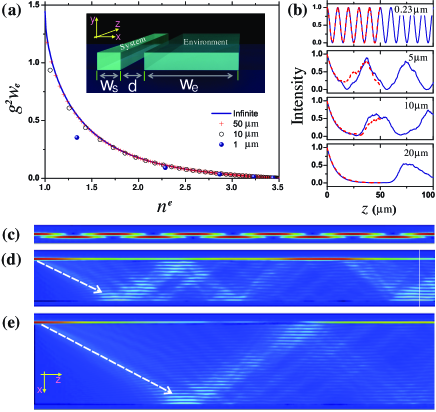
Figure 1: (Color online) (a) The normalized coupling strength $g^{2}w_{e}$ between system and environment against effect mode index $n^{e}$ for different environment size $w_{e}$. Inset: schematic illustration of the coupled photonic waveguides simulation to the system-environment interaction. (b) Typical dynamics of system energy against the interaction length $z$ for different $w_{e}$, with the solid and dashed lines are analytical and numerical results. (c)-(e) False-color profiles of electric field intensity for light loaded in the system waveguide at $z=0$, with $d=0.15\mu m$ and $w_{e}=0.23,5,10$ $\mu m,$ respectively.

Model.- As illustrated by the Inset of Fig. 1(a), the proposed photonic simulation of the system-environment interaction is composed of two separated waveguides. Photon can be loaded at system waveguide and travel along it ($z$-axis). The system is open because its energy can dissipate to the nearby waveguide which acts as environment. The dynamics of photon in single isolated waveguide can be described by the Helmholtz equations as (Yariv, 1989)

$$\nabla^{2}\psi(\overrightarrow{r})+V(\overrightarrow{r})\psi(\overrightarrow{r})=E\psi(\overrightarrow{r}),$$ (1)

where $V(\overrightarrow{r})=[\varepsilon(\overrightarrow{r})-1]k^{2}$ and $E=k^{2}$, with the dielectric relative permittivity $\varepsilon(\overrightarrow{r})$ and the wave-number $k=2\pi/\lambda$. The waveguides are uniform along the $z$-axis. Therefore the $i$-th propagating eigenmode’s wave function can be expressed as $\psi_{i}(\overrightarrow{r})=\varphi_{i}(\overrightarrow{x})e^{in_{i}kz}$, where $\varphi_{i}(\overrightarrow{x})$ is the field distribution at the cross section of a waveguide, and $n_{i}$ is the effective mode index which can be solved from the characteristic equation. For coupled system and environment waveguides, we can decompose any field distribution perturbatively as

$$\psi(\overrightarrow{r})=\sum_{i}c_{i}^{s}(z)\psi_{i}^{s}(\overrightarrow{r})+\sum_{j}c_{j}^{e}(z)\psi_{j}^{e}(\overrightarrow{r}),$$ (2)

where superscript s and e denote system and environment waveguides, respectively. Here, $i=1,...,N_{s}$, $j=1,...,N_{e}$, with $N_{s(e)}$ is the number of modes in the system (environment) waveguides. $\psi_{i}^{s}(\overrightarrow{r})$ and $\psi_{j}^{e}(\overrightarrow{r})$ are eigenmodes of waveguides, and $c_{i}^{s}(z)$ and $c_{j}^{e}(z)$ are corresponding coefficients. Substituting $V(\overrightarrow{r})=V^{s}(\overrightarrow{r})+V^{e}(\overrightarrow{r})$ and $\psi(\overrightarrow{r})$ to Eq. (1), we can obtain the dynamics of the modes in each waveguide as

$$i\frac{\partial c_{i}^{s(e)}}{\partial z} =\sum_{l}m_{il}^{s(e)}e^{i(n_{i}^{s(e)}-n_{l}^{s(e)})kz}c_{l}^{s(e)}$$

$$+\sum_{j}g_{ij}^{s(e)}e^{i(n_{i}^{s(e)}-n_{j}^{e(s)})kz}c_{j}^{e(s)},$$ (3)

where coupling efficiencies $m_{il}^{s(e)}=\frac{\int(\varphi_{i}^{s(e)})^{\ast}V^{s(e)}\varphi_{l}^{s(e)}d\overrightarrow{x}}{2n_{i}^{s(e)}k}$ and $g_{ij}^{s(e)}=\frac{\int(\varphi_{i}^{s(e)})^{\ast}V^{s(e)}\varphi_{j}^{e(s)}dx}{2n_{i}^{s(e)}k}$, with all wave functions are normalized by $\int\left|\varphi_{i}^{s(e)}\right|^{2}dx=1$.

Considering a thin system waveguide that supports only one guiding mode ($N_{s}=1$), while the number of modes of the environment waveguide $N_{e}\geq 1$ which depends on its width $w_{e}$. Denoting the system and environment fields by $a=c_{1}^{s}e^{-in_{1}^{s}kz}$ and $b_{j}=\sqrt{g_{1j}^{s}/g_{1j}^{e}}c_{j}^{e}e^{-in_{j}^{e}kz}$ ($j=1,...,N_{e}$) respectively, and replacing the space coordinate $z$ by time $t$, we can obtain the Hamiltonian which governs the dynamics of this photonic simulation of the system-environment interaction as ($\hbar=1$)

$$H=\beta_{0}a^{{\dagger}}a+\sum_{j}\beta_{j}b_{j}^{{\dagger}}b_{j}+\sum_{j}g_{j}(a^{{\dagger}}b_{j}+ab_{j}^{{\dagger}}),$$ (4)

where $\beta_{0}=(n_{1}^{s}+m_{11}^{s})k=n_{0}k$ and $\beta_{j}=(n_{j}^{e}+m_{jj}^{e})k=n_{j}k$ are propagation constants, and $g_{j}=\sqrt{g_{1j}^{s}g_{1j}^{e}}$ is the coupling coefficients. Since the direct coupling between environment modes is much smaller than other terms, $m_{i,j}^{e}$ ($i\not=j$) is neglected in following studies.

Non-Markovian and Markovian Processes.- The Hamiltonian of Eq. (4) resembles an open system that a harmonic oscillator ($a$) couples to a collection of oscillators in environment ($b_{j}$). Here, both the coupling coefficients and the environment can be well controlled, which is very promising to simulate the system-environment interaction. With two-dimensional approximation, $\beta_{j}$ and $g_{j}$ can be solved analytically. In the following, we studied the model with photonic waveguides made of silicon $(n_{d}=3.5)$, which have been extensively studied in practical experiments. The working wavelength $(\lambda)$ is $1550\mathrm{nm}$, and the width of system waveguide is fixed to $w_{s}=0.23\mathrm{\mu m}$ in the single mode regime.

The normalized coupling strength ($g^{2}w_{e}$) between system and environment against mode index $n^{e}=\beta_{j}/k$ is shown in Fig. 1(a). The continuum of finite size environment is quantized to discrete modes, whose density and number $N_{e}$ increases with $w_{e}$. The behaviors of $g^{2}w_{e}$ converges to a line with infinite $N_{e}$ when $w_{e}$=$\infty$, which corresponds to system-reservoir interaction. With these parameters, the dynamics of the system and environment can be solved according to Eq. (4). In Fig. 1(b), the evolutions of energy in system waveguide against $z$ for different $w_{e}$ are calculated, with light loaded in the system waveguide at $z=0$. For a comparison, the fields in system are also simulated numerically by finite element method. The results of our analytical method agree very well with numerical results, with small discrepancies originating from the slow varying and weak coupling approximations used in our analytical expressions. For small environment ($w_{e}=0.23\mu m$ and $5\mu m$), the dynamics of the system shows periodic oscillation. When the environment size increases, the dynamics changes: the system energy shows exponential decay at first and revives after a distance.

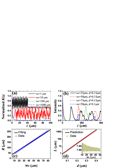
Figure 2: (Color online) (a) The memory kernel function for different environment sizes, with $d=0.15\mu m$. (b) The dynamics of system for different $w_{e}$ and $d$. (c) The revival period $R$ against $w_{e}$, with dots obtained from the system dynamics, and solid line from the analytical model, with $d=0.15\mu m.$ (d) The decay length against $d$, with dots and line being results of the system dynamics and analytical model with $w_{e}=\infty$. Inset: the decay length against $w_{e}$ obtained from the system dynamics.

A direct view of the dynamics of the coupled system-environment can be clearly observed in Fig. 1(c)-(e). When $w_{e}$ is comparable with $\lambda$, there is few modes can be involved to interaction with the system, the coherent coupling of which leads to sinusoidal oscillation of system energy [Fig. 1(c)]. For larger $w_{e}$, more modes could interact with the system, giving rise to a complex dynamics. It is interesting that the corporation of environment modes shows a classical ray trajectory of light leaked from the system waveguide, as indicated by the dashed line in Fig. 1(d), with an incident angle $\chi=\mathrm{arcsin}(\beta_{0}/k)$ with respect to $z$-axis. For $w_{e}\geq 10\mu m$, the energy exponentially decays with $z$ and can almost completely leak into environment [Fig. 1(e)]. And after a certain distance, the leakage will be reflected into system and cause a revival of system.

Furthermore, some important interaction properties to understand the underlying physics can be easily obtained from those figures. The formal solution of the dynamics of system $a(z)$ is derived in the interaction picture $H_{I}(z)=\sum_{j}\hbar g_{j}(a^{{\dagger}}b_{j}e^{i(\beta_{0}-\beta_{j})z}+ab_{j}^{{\dagger}}e^{-i(\beta_{0}-\beta_{j})z})$ by employing the formal solution $b_{j}(z)=-ig_{j}\int_{0}^{z}a(\tau)e^{-i(\beta_{0}-\beta_{j})\tau}d\tau$ . The dynamics of system reads

$$\frac{\partial}{\partial z}a(z)=-\int_{0}^{z}a(\tau)K(\tau-z)d\tau,$$ (5)

with the memory kernel function $K(\tau)=\sum_{j}g_{j}^{2}e^{-i(\beta_{0}-\beta_{j})\tau}$ (Breuer and Petruccione, 2002). For small $w_{e}$, the beating of multiple environment modes gives rise to the oscillation behavior of $K(\tau)$. The non-zero memory effect leads to non-Markovian dynamics of system, showing non-exponential energy decay and revival phenomenon [as shown in Fig. 1(b)]. Since the period of $K(\tau)$ is determined by the environment mode density $\rho(n)\approx\frac{kw_{e}}{\pi}\frac{n}{\sqrt{n_{d}^{2}-n{}^{2}}}$, the non-Markovian revival period linearly depends on $w_{e}$, which can be observed in Fig. 2(b). We can also deduce the revival period $R=2w_{e}\mathrm{tan}\chi+R_{0}$ with intuitive understanding of revival as beam reflection at boundary of environment. The revival period extracted from the dynamics of system shown in Fig. 2(c) are well fitted by this formula. The constant $R_{0}$ is corresponding to an extra distance required for tunneling (Hauge and Støvneng, 1989) and Goos-Hänchen shift (Snyder and Love, 1976) of light when reflecting at the environment boundary.

Fig. 2(a) shows that $K(\tau)$ becomes the Dirac delta function $\delta(\tau)$ when the environment size approaches to infinity. As a great many environment modes are involved when $w_{e}\rightarrow\infty$, the memory kernel function can be approximately written in the form of integration $K(\tau)=\int g^{2}(n)e^{-i(\beta_{0}-nk)\tau}\rho(n)dn$, where the coupling strength $g(n)$ is a function of mode index $n$ [Fig. 1(a)]. Then

$$K(\tau)\approx J(n_{0})\delta(\tau),$$ (6)

where $n_{0}=\beta_{0}/k$ and $J(n)=g^{2}(n)w_{e}\frac{n}{\sqrt{n_{d}^{2}-n^{2}}}$ is the spectrum density function of the reservoir. This $\delta(\tau)$ memory function gives rise to the Markovian process that system energy decays exponentially as $a(z)=e^{-z/2L}$. The decay length

$$L=\frac{1}{2J(n_{0})}\approx L_{0}e^{-2\sqrt{\beta_{0}^{2}-k^{2}}d},$$ (7)

where $L_{0}=\frac{1}{k}\frac{n_{0}(n_{d}^{2}-1)^{2}(kw_{s}+2/\sqrt{n_{0}^{2}-1})}{8(n_{0}^{2}-1)(n_{d}^{2}-n_{0}^{2})^{3/2}}$ is solved explicitly. In Fig. 2(d), the analytical decay length is compared to the results extracted from the dynamics of system with logarithmic fitting. Our prediction is consistent with the data, and the slight discrepancy is due to non-flat noise spectrum density [Eq. (6)]. It is surprising that the formula of $L$ in the continuum limit works for small $w_{e}$, as shown in the inset of Fig. 2(d). The oscillation of which is due to the variation of mode index of discrete modes in finite environment.

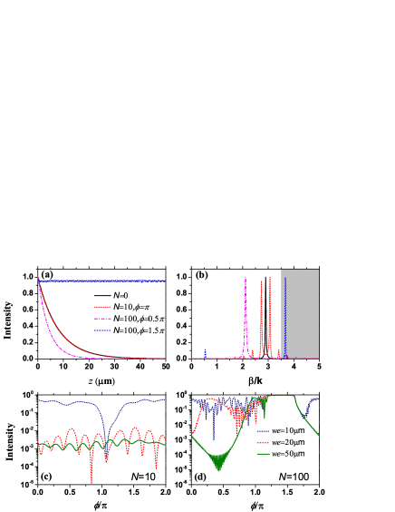
Figure 3: (Color online) The system evolution (a) and corresponding spectrum (b) when a sequence of $N$ modulation of phase $\phi$ applied to the system. (c) and (d) The system energy at $z=50\mu m$ against $\phi$ for different $w_{e}$ and $N$, with $d=0.15\mu m$.

Dynamical Decoupling.- It is well known that external modulation to open quantum systems can modify the energy decay and decoherence, and the so-called “dynamical decoupling” technique has been widely adopted to keep the coherence of electron spins (Viola et al., 1999; Du et al., 2009; De Lange et al., 2010). Similarly, for the photonic simulation of system-environment interaction, a dynamical modulation of system waveguide can also alter the energy decay. Here, a sequence of $N$ modulations with equal interval is applied to the system waveguide, where each modulation corresponds to an abrupt change of phase $\phi$. Fig. 3(a) shows the evolution of system changes when modulation is applied. The dissipation of system can be enhanced or inhibited significantly depending on $\phi$ and $N$. As shown by Fig. 3(c) and (d) are energy in the system waveguide at $z=50\mu m$ against the modulation phase $\phi$, with different $w_{e}$ and $N$.

There’s an intuitive way to understand the modified decay: The modulations add extra phase to the propagating light, which is equivalent to an increase or decrease of the effective index $\widetilde{n}$, as the phase of propagating photon is proportional to $\widetilde{n}$. As shown in Fig. 3(b), the spectrum of the system is shifted by the modulations. According to the spectrum density of reservoir [Fig. 1(a)], different $\widetilde{n}$ corresponds to different coupling strength, then the modulations give rise to acceleration or deceleration of dissipation. When $\widetilde{n}$ is larger than the cut-off index $n_{d}$, the dissipation of energy in system to the environment is forbidden. From another point of view, the waveguide with periodic modulation is similar to the photonic crystal or grating structures, which will induce a band structure to the light. By this means, noise in environment can be prevented from propagating in system. These provide physics insight to the dynamical decoupling in time dimension where a sequence of modulation in time-axis is applied: the effective frequency of the system shifts to a higher value than the cut-off frequency of bath. Or, we can image a crystal or band structure in time dimension, where only the signal with certain frequencies can enter and be kept in the system while most of the broadband noises in environment is blocked.

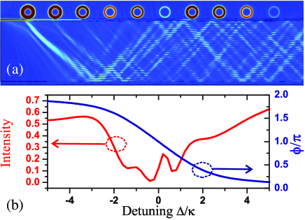
Figure 4: (Color online) (a) The fields of system and environment when microdisks are added to the waveguide to induce a phase modulation. (b) The dynamics against the detuning of input light to the whispering gallery modes.

One possible way to realize such phase modulation sequence is shown in Fig. 4(a), with whispering gallery mode (WGM) microdisks coupling to the system waveguide (Cai et al., 2000). The microdisk with radius $r=1\mu m$ has intrinsic quality factor higher than $10^{6}$. When put close to the system waveguide with a gap ($0.15\mu m$), its loaded quality factor is only about $2000$. That means the WGM is working in the strongly over coupling regime with $\kappa_{e}\gg\kappa_{i}$, where $\kappa_{i(e)}$ is the intrinsic (external) loss. When the light in system passes the over-coupled WGM resonator, the change of transmitted light is $T(\Delta)=-\frac{1-i\Delta/(\kappa_{e}-\kappa_{i})}{1+i\Delta/(\kappa_{e}+\kappa_{i})}\approx-\frac{1-i\Delta/\kappa_{e}}{1+i\Delta/\kappa_{e}}$, where $\Delta$ is the frequency detuning to the resonance. As $|T(\Delta)|\approx 1$, the system acquires a modulation of phase $\phi(\Delta)=\mathrm{arg}[T(\Delta)]$. Numerical simulation of the dynamical decoupling with $N=10$ for $w_{e}=10\mu m$ is performed. Comparing the mode profile of Fig. 4(a) with Fig. 1(e), the evolutions are significantly changed by modulations. From Fig. 4(b), a strong modification of the decay is shown around the resonance that phase modulation $\phi\approx\pi$, which is consistent with the prediction in Fig. 3(a).

Conclusion.- The Markovian, non-Markovian processes and dynamic decoupling of open quantum systems are studied in a photonic simulation of system-environment interaction. Intuitive physical insight and deep understanding of these phenomena can be gained from the direct view of electromagnetic field profiles. Our study also opens the possibility to tune the dissipation in photonic system, similar to the dynamic decoupling of spins.

Acknowledgments This work was supported by the 973 Programs (No.2011CB921200 and No. 2011CBA00200), the National Natural Science Foundation of China (NSFC) (No. 11004184), the Knowledge Innovation Project of the Chinese Academy of Sciences (CAS).

References

- Breuer and Petruccione (2002) H. P. Breuer and F. Petruccione, The theory of open quantum systems (Oxford University Press, New York, 2002).
- Zurek (2003) W. H. Zurek, Rev. Mod. Phys. 75, 715 (2003).
- Fischer et al. (2001) M. Fischer, B. Gutiérrez-Medina, and M. Raizen, Phys. Rev. Lett. 87, 40402 (2001).
- Koshino and Shimizu (2005) K. Koshino and A. Shimizu, Phys. Rep. 412, 191 (2005).
- Liu et al. (2011) B.-H. Liu, L. Li, Y.-F. Huang, C.-F. Li, G.-C. Guo, E.-M. Laine, H.-P. Breuer, and J. Piilo, Nature Phys. 7, 931 (2011).
- Wolf et al. (2008) M. M. Wolf, J. Eisert, T. S. Cubitt, and J. I. Cirac, Phys. Rev. Lett. 101, 150402 (2008).
- Diehl et al. (2008) S. Diehl, A. Micheli, A. Kantian, B. Kraus, H. Büchler, and P. Zoller, Nature Phys. 4, 878 (2008).
- Verstraete et al. (2009) F. Verstraete, M. Wolf, and J. Cirac, Nature Phys. 5, 633 (2009).
- Barreiro et al. (2010) J. Barreiro, P. Schindler, O. Gühne, T. Monz, M. Chwalla, C. Roos, M. Hennrich, and R. Blatt, Nature Phys. 6, 943 (2010).
- Krauter et al. (2011) H. Krauter, C. Muschik, K. Jensen, W. Wasilewski, J. Petersen, J. Cirac, and E. Polzik, Phys. Rev. Lett. 107, 80503 (2011).
- Viola et al. (1999) L. Viola, E. Knill, and S. Lloyd, Phys. Rev. Lett. 82, 2417 (1999).
- Du et al. (2009) J. Du, X. Rong, N. Zhao, Y. Wang, J. Yang, and R. Liu, Nature 461, 1265 (2009).
- De Lange et al. (2010) G. De Lange, Z. Wang, D. Riste, V. Dobrovitski, and R. Hanson, Science 330, 60 (2010).
- Buluta and Nori (2009) I. Buluta and F. Nori, Science 326, 108 (2009).
- Bloch et al. (2012) I. Bloch, J. Dalibard, and S. Nascimbène, Nature Phys. 8, 267 (2012).
- Aspuru-Guzik and Walther (2012) A. Aspuru-Guzik and P. Walther, Nature Phys. 8, 285 (2012).
- Feynman (1982) R. Feynman, Int. J. Theor. Phys. 21, 467 (1982).
- Barreiro et al. (2011) J. Barreiro, M. Müller, P. Schindler, D. Nigg, T. Monz, M. Chwalla, M. Hennrich, C. Roos, P. Zoller, and R. Blatt, Nature 470, 486 (2011).
- Hafezi et al. (2011) M. Hafezi, E. Demler, M. Lukin, and J. Taylor, Nature Phys. 7, 907 (2011).
- Longhi (2009) S. Longhi, Laser & Photon. Rev. 3, 243 (2009).
- Garanovich et al. (2012) I. Garanovich, S. Longhi, A. Sukhorukov, and Y. Kivshar, Phys. Rep. 518, 1 (2012).
- Yariv (1989) A. Yariv, Quantum Electronics (Wiley and Sons, New York, 1989).
- Hauge and Støvneng (1989) E. Hauge and J. Støvneng, Rev. Mod. Phys. 61, 917 (1989).
- Snyder and Love (1976) A. Snyder and J. Love, Appl. Opt. 15, 236 (1976).
- Cai et al. (2000) M. Cai, O. Painter, and K. Vahala, Phys. Rev. Lett. 85, 74 (2000).