Adaptive Thouless-Anderson-Palmer approach to inverse Ising problems with quenched random fields

Abstract

The adaptive Thouless-Anderson-Palmer equation is derived for inverse Ising problems in the presence of quenched random fields. We test the proposed scheme on Sherrington-Kirkpatrick, Hopfield, and random orthogonal models and find that the adaptive Thouless-Anderson-Palmer approach allows surprisingly accurate inference of quenched random fields whose distribution can be either Gaussian or bimodal, compared with other existing mean-field methods.

I Introduction

The inverse Ising problem has been intensively studied in statistical physics and computational biology in the past few years Schneidman et al. (2006); Weigt et al. (2009); Bailly-Bechet et al. (2010); Cocco and Monasson (2012). Such studies are of huge practical and theoretical relevance. On one hand, the advent of techniques for multi-electrode recording and microarray measurement produces high-throughput biological data Stevenson and Kording (2011). Unveiling the biological mechanism underlying these experimental data poses a challenging computational problem. In the inverse Ising problem, one tries to construct a statistical mechanics description of the original system directly from the data, and it provides a promising tool for dimensional reduction in modeling vast amounts of biological data Mora and Bialek (2011). On the other hand, for guaranteeing the reliability of the obtained description, it is also necessary to examine the reconstruction performance of the inverse algorithms numerically and/or analytically by utilizing artificial data that are generated from a variety of known Ising spin models Tanaka (1998); Roudi et al. (2009); Cocco and Monasson (2012); Mastromatteo and Marsili (2011); Cocco and Monasson (2011).

In general, the experimental data are described by $M$ independent samples $\{\boldsymbol{\sigma}^{1},\boldsymbol{\sigma}^{2},\ldots,\boldsymbol{\sigma}^{M}\}$ in which $\boldsymbol{\sigma}$ is an $N$-dimensional vector with binary components ($\sigma_{i}=\pm 1$) and $N$ is the system size. The Ising model provides the least structured model to match the statistics of the experimental data as

$$P_{{\rm Ising}}(\boldsymbol{\sigma})=\frac{1}{Z(\mathbf{h},\mathbf{J})}\exp\left[\sum_{(ij)}J_{ij}\sigma_{i}\sigma_{j}+\sum_{i}h_{i}\sigma_{i}\right],$$ (1)

where $(ij)$ denotes all distinct spin pairs and the partition function $Z(\mathbf{h},\mathbf{J})$ depends on $N$-dimensional fields and $\frac{N(N-1)}{2}$-dimensional couplings. These fields and couplings are chosen to yield the same first and second moments (magnetizations and pairwise correlations, respectively) as those obtained from the experimental data. The inverse temperature $\beta\equiv 1/T$ is absorbed into the strength of fields and couplings.

Based on magnetizations and correlations, the inference of fields and couplings of the Ising model is a computationally hard problem especially for large systems. However, one can resort to mean-field methods, such as naive mean-field (nMF) Kappen and Rodriguez (1998), Thouless-Anderson-Palmer (TAP) equation Tanaka (1998), Sessak-Monasson (SM) expansion Sessak and Monasson (2009), and Bethe approximation (BA) Mézard and Mora (2009); Ricci-Tersenghi (2012); Nguyen and Berg (2012), to get an approximate solution to the inverse problem with computationally feasible costs. Previous investigations have mostly focused on the inference of the coupling vector, whereas the inference error of fields has been less analyzed. In fact, external fields represent intrinsically preferred directions of $\{\sigma_{i}\}$, which are also very important for understanding information processing in real neuronal networks Schneidman et al. (2006); Huang and Zhou (2012) and gene interaction networks Bailly-Bechet et al. (2010) and for predicting protein structures from sequence data Weigt et al. (2009); Marks et al. (2011). Therefore, an accurate estimation of external fields is also highly desirable.

To this end, we propose the adaptive Thouless-Anderson-Palmer (adaTAP) approach for the inverse Ising problem and establish the framework on the basis of Gibbs free energy and Gaussian approximation. Surprisingly, adaTAP yields a very accurate estimation of external fields, although some other mean-field methods are more competitive in predicting couplings. We confirm the efficiency of adaTAP on three kinds of mean-field models: the Sherrington-Kirkpatrick (SK) model Sherrington and Kirkpatrick (1975), the Hopfield Amit et al. (1987) model and the random orthogonal model (ROM) Parisi and Potters (1995); other existing mean-field inverse algorithms are also compared.

The outline of this paper is as follows. The adaptive TAP approach to the inverse Ising problem with quenched random fields is derived in Sec. II. In Sec. III, extensive numerical simulations are carried out to test the inference performance of adaTAP on Hopfield model, SK model and ROM. The comparison with other existing mean-field methods is also made and discussed. Concluding remarks are given in Sec. IV.

II Adaptive TAP approach

For the Ising model defined in Eq. (1), we write the magnetization-dependent free energy (also termed Gibbs free energy) as

$$G(\mathbf{m})=-\mathbf{h}^{T}\mathbf{m}+{\rm Extr}_{\boldsymbol{\theta}}\left\{\boldsymbol{\theta}^{T}\mathbf{m}-\ln\sum_{\boldsymbol{\sigma}}e^{\frac{1}{2}\boldsymbol{\sigma}^{T}\mathbf{J}\boldsymbol{\sigma}+\boldsymbol{\theta}^{T}\boldsymbol{\sigma}}\right\},$$ (2)

where the Lagrange multiplier vector $\boldsymbol{\theta}$ is introduced to fix magnetizations at all sites to their thermal expectation values, i.e., $m_{i}=\left<\sigma_{i}\right>$. $\mathbf{h}^{T}$ denotes the transpose of a vector $\mathbf{h}$. The notation ${\rm Extr}$ stands for the extremum with respect to the corresponding parameters ($\boldsymbol{\theta}$ here). The exact evaluation of the partition function in Eq. (2) is computationally difficult for a large system. However, one can resort to mean-field approximations. We adopt the following strategy. First, each coupling is multiplied by a real number $l\in[0,1]$, and the Gibbs free energy can then be expressed by

$$\begin{split}G(\mathbf{m})&=G(\mathbf{m},l=1)=\int_{0}^{1}dl\frac{\partial G(\mathbf{m},l)}{\partial l}+G(\mathbf{m},l=0)\\ &\simeq G_{{\rm g}}(\mathbf{m},l=1)-G_{{\rm g}}(\mathbf{m},l=0)+G(\mathbf{m},l=0),\end{split}$$ (3a)

$$G(\mathbf{m},l) =-\mathbf{h}^{T}\mathbf{m}+{\rm Extr}_{\boldsymbol{\theta}}\left\{\boldsymbol{\theta}^{T}\mathbf{m}-\ln\sum_{\boldsymbol{\sigma}}e^{\frac{l}{2}\boldsymbol{\sigma}^{T}\mathbf{J}\boldsymbol{\sigma}+\boldsymbol{\theta}^{T}\boldsymbol{\sigma}}\right\},$$ (3b)

$$\begin{split}G_{{\rm g}}(\mathbf{m},l)&=-\mathbf{h}^{T}\mathbf{m}+{\rm Extr}_{\boldsymbol{\theta},\boldsymbol{\Lambda}}\Biggl{\{}\boldsymbol{\theta}^{T}\mathbf{m}-\frac{1}{2}{\rm tr}(\boldsymbol{\Lambda}\mathbf{\tilde{C}})\\ &-\ln\int d\boldsymbol{\sigma}e^{-\frac{1}{2}\boldsymbol{\sigma}^{T}(\boldsymbol{\Lambda}-l\mathbf{J})\boldsymbol{\sigma}+\boldsymbol{\theta}^{T}\boldsymbol{\sigma}}\Biggr{\}},\end{split}$$ (3c)

where $\tilde{C}_{ij}\equiv\left<\sigma_{i}\sigma_{j}\right>$, and we have used Gaussian statistics for the binary spins with expectation constraints, i.e., $\left<\sigma_{i}\sigma_{j}\right>_{{\rm g}}=\left<\sigma_{i}\sigma_{j}\right>_{{\rm Ising}}$ which are enforced by a symmetric matrix $\boldsymbol{\Lambda}$. Here, ${\rm tr}(\mathbf{A})$ denotes the trace of a matrix $\mathbf{A}$. For simplicity, we assume $\boldsymbol{\Lambda}$ is a diagonal matrix $\boldsymbol{\Lambda}={\rm diag}(\Lambda_{1},\ldots,\Lambda_{N})$ whose diagonal terms are determined via the extremization of the corresponding Gibbs free energy. The Gaussian approximation makes the computation of the partition function tractable. This scheme is also called the expectation consistence approximation Heskes et al. (2005) and was applied to derive the message-passing algorithm for the perceptron learning problem Shinzato and Kabashima (2008). Conventional Plefka expansion Plefka (1982) truncates the power series expansion of $G(\mathbf{m},l)$ to second order in $l$, but Eq. (3a) contains terms of all orders. Note that the third term in Eq. (3a) is the Gibbs free energy of non-interacting Ising spins at fixed magnetizations and can be easily evaluated. The final expression for the Gibbs free energy reads,

$$\begin{split}G(\mathbf{m})&\simeq-\frac{1}{2}\mathbf{m}^{T}\mathbf{J}\mathbf{m}-\mathbf{h}^{T}\mathbf{m}+\sum_{i}\mathcal{H}(m_{i})+\frac{1}{2}\ln{\rm det}(\boldsymbol{\Lambda}-\mathbf{J})\\ &-\frac{1}{2}\sum_{i}(1-m_{i}^{2})\Lambda_{i}+\frac{1}{2}\left(N+\sum_{i}\ln(1-m_{i}^{2})\right),\end{split}$$ (4)

where $\mathcal{H}(m_{i})\equiv\frac{1+m_{i}}{2}\ln\frac{1+m_{i}}{2}+\frac{1-m_{i}}{2}\ln\frac{1-m_{i}}{2}$ and $\boldsymbol{\Lambda}$ follows the extremization condition of Eq. (3c) with $l=1$,

$$(\boldsymbol{\Lambda}-\mathbf{J})^{-1}_{ii}=1-m_{i}^{2}.$$ (5)

Equilibrium values of magnetizations are determined by $\mathbf{m}_{{\rm eq}}={\rm argmin}_{\mathbf{m}}G(\mathbf{m})$ and the free energy $F=\min_{\mathbf{m}}G(\mathbf{m})$. A quick calculation gives the self-consistent equation for $\mathbf{m}$,

$$m_{i}=\tanh\left[h_{i}+\sum_{j}J_{ij}m_{j}-m_{i}\left(\Lambda_{i}-\frac{1}{1-m_{i}^{2}}\right)\right],$$ (6)

which is exactly the adaptive TAP equation first introduced in Refs. Opper and Winther (2001a, b) for the Ising model. Eq. (6) can also be derived under other mean-field approximations Raymond and Ricci-Tersenghi (2012, 2013); Yasuda and Tanaka (2013). The third term inside the square bracket of Eq. (6) forms the Onsager correction term which requires no prior knowledge of the coupling statistics, playing an important role in inferring external fields. $\Lambda_{i}$ in Eq. (6) is a function of $\{m_{i}\}$ determined by Eq. (5). The fixed point of the self-consistent equation gives $\mathbf{m}_{\rm eq}$. We remark here that Eq. (6) can be reduced to the normal TAP equation obtained from a high-temperature expansion of the Gibbs free energy Plefka (1982); Georges and Yedidia (1991); Yasuda et al. (2012), i.e., the third term inside the square bracket of Eq. (6) becomes $-m_{i}\sum_{j}(1-m_{j}^{2})J_{ij}^{2}$ (Onsager reaction term) through high-temperature expansion.

To obtain the inference equations for couplings, we use the identity $\mathbf{H}\mathbf{C}=\mathbf{I}$ Bray and Moore (1979); Tanaka (1998); Yasuda and Tanaka (2009) where $\mathbf{H}$ is the Hessian matrix of the Gibbs free energy $H_{ij}\equiv\frac{\partial^{2}G}{\partial m_{i}\partial m_{j}}$ and $\mathbf{C}$ is the connected correlation matrix whose entries are $C_{ij}\equiv\left<\sigma_{i}\sigma_{j}\right>-m_{i}m_{j}$. $\mathbf{I}$ is an identity matrix. Magnetizations and correlations are already given by the experimental data in the inverse Ising problem. Finally, the inference equation reads

$$J_{ij}=-(\mathbf{C}^{-1})_{ij}+m_{i}(\mathbf{B}^{-1})_{ij}$$ (7)

for $i\neq j$, where $B_{ij}\equiv\frac{1}{2m_{i}}\left[\chi_{ij}\right]^{2}$ which expresses how large the change of $m_{i}$ is given a small perturbation to $\Lambda_{j}$ and we define $\boldsymbol{\chi}=(\boldsymbol{\Lambda}-\mathbf{J})^{-1}$. The expression for $B_{ij}$ is derived by using the Sherman-Morrison formula Press et al. (2007). A small perturbation $\Delta\Lambda_{j}$ to $\Lambda_{j}$ will lead to a corresponding change of $m_{i}$ according to Eq. (5), which is described by the following equation:

$$[\boldsymbol{\chi}^{-1}+\Delta\boldsymbol{\Lambda}_{j}]_{ii}^{-1}=\chi_{ii}-\frac{\Delta\Lambda_{j}\chi_{ij}^{2}}{1+\Delta\Lambda_{j}\chi_{ij}}\\ =1-(m_{i}+\Delta m_{i})^{2},$$ (8)

where the Sherman-Morrison formula is used in the first equality and the notation $\Delta\boldsymbol{\Lambda}_{j}$ means that only $j$-th diagonal term of matrix $\Delta\boldsymbol{\Lambda}$ is non-zero and equal to $\Delta\Lambda_{j}$. Noting that both $\Delta m_{i}$ and $\Delta\Lambda_{j}$ are small, one can obtain $B_{ij}\equiv\frac{\partial m_{i}}{\partial\Lambda_{j}}=\frac{1}{2m_{i}}\left[\chi_{ij}\right]^{2}$ by using Eq. (5) once again. After couplings are reconstructed, external fields are inferred as

$$h_{i}=\tanh^{-1}(m_{i})-\sum_{j}J_{ij}m_{j}+m_{i}\left(\Lambda_{i}-\frac{1}{1-m_{i}^{2}}\right).$$ (9)

To predict the coupling, we need to solve the adaTAP equation Eq. (5). An iterative scheme is proposed as follows.

Step 1.

Let $t=0$ and initialize $J_{ij}=-(\mathbf{C^{-1}})_{ij}$, $\Lambda_{i}=(1-m_{i}^{2})^{-1}$ for all $(ij)$ and $i$ respectively.

Step 2.

At $t$, set $t^{\prime}=0$, $\tilde{\boldsymbol{\Lambda}}^{t^{\prime}=0}=\boldsymbol{\Lambda}^{t}$, $\boldsymbol{\chi}=(\boldsymbol{\Lambda}^{t}-\mathbf{J}^{t})^{-1}$.

Step 2.1.

$t^{\prime}\leftarrow t^{\prime}+1$, update $\tilde{\Lambda}^{t^{\prime}}_{i}=\tilde{\Lambda}^{t^{\prime}-1}_{i}+\Delta\tilde{\Lambda}_{i}$ where $\Delta\tilde{\Lambda}_{i}=\frac{1}{1-m_{i}^{2}}-\frac{1}{\chi_{ii}}$ for all $i$. After update of each $\tilde{\Lambda}^{t^{\prime}}_{i}$, $\boldsymbol{\chi}$ needs to be updated simultaneously as $\chi_{kl}^{{\rm new}}=\chi_{kl}^{{\rm old}}-\frac{\chi_{ki}^{{\rm old}}\Delta\tilde{\Lambda}_{i}\chi_{il}^{{\rm old}}}{1+\Delta\tilde{\Lambda}_{i}\chi_{ii}^{{\rm old}}}$ derived by using the Sherman-Morrison formula.

Step 2.2

Until $|\Delta\tilde{\Lambda}_{i}|<\epsilon_{\Lambda}$ for all $i$, then assign $\boldsymbol{\Lambda}^{t}=\tilde{\boldsymbol{\Lambda}}^{t^{\prime}}$, $\boldsymbol{\chi}^{t}=\boldsymbol{\chi}$ and go to Step 3. Otherwise, if $t^{\prime}<t^{\prime}_{{\rm max}}$, go to Step 2.1, else return UN-CONVERGED.

Step 3.

$t\leftarrow t+1$, update $J_{ij}^{t}=-(\mathbf{C}^{-1})_{ij}+m_{i}(\mathbf{B}^{-1})_{ij}$ where $B_{ij}\equiv\frac{1}{2m_{i}}\left[\chi^{t-1}_{ij}\right]^{2}$, until $|J_{ij}^{t}-J_{ij}^{t-1}|<\epsilon_{J}$ for all $(ij)$, then go to Step 4. Otherwise, if $t<t_{{\rm max}}$, go to Step 2, else return UN-CONVERGED.

Step 4.

Infer $h_{i}$ according to Eq. (9) for all $i$.

In step 2.1, the step size $\Delta\tilde{\Lambda}_{i}$ for updating $\tilde{\Lambda}_{i}$ can be derived by using Eq. (5) and the Shermon-Morrison formula, which gives $\chi_{ii}-\frac{\Delta\tilde{\Lambda}_{i}\chi_{ii}^{2}}{1+\Delta\tilde{\Lambda}_{i}\chi_{ii}}=1-m_{i}^{2}$. In the iterative scheme, we set the parameters $t_{{\rm max}}=t^{\prime}_{{\rm max}}=1000$, and $\epsilon_{\Lambda}=\epsilon_{J}=10^{-4}$. In practice, we find that both $\boldsymbol{\Lambda}$ and $\mathbf{J}$ in our simulations shown below converge in tens of steps when the temperature is not very low. The computational complexity of this iterative scheme is dominated by the inverse of the matrix (e.g., $\mathbf{C}$ or $\mathbf{B}$), keeping the same order as that of other mean-field methods.

To compare performances of different mean-field inverse algorithms, we define the inference error for couplings and fields, respectively, as

$$\Delta_{J} =\left[\frac{2}{N(N-1)}\sum_{i<j}(J_{ij}^{*}-J_{ij}^{{\rm true}})^{2}\right]^{1/2},$$ (10a)

$$\Delta_{h} =\left[\frac{1}{N}\sum_{i}(h_{i}^{*}-h_{i}^{{\rm true}})^{2}\right]^{1/2},$$ (10b)

where $J_{ij}^{*}$ ($h_{i}^{*}$) is the inferred coupling (field) and $J_{ij}^{{\rm true}}$ ($h_{i}^{{\rm true}}$) is the true one.

III Numerical simulations

We evaluate the inference performance of the adaTAP approach on three mean-field models with either Gaussian distributed or bimodal distributed random fields. For the SK model, each entry of the coupling matrix are independently drawn at random from a Gaussian distribution with zero mean and variance $1/N$. In the Hopfield model, the coupling is constructed according to Hebb’s rule, i.e., $J_{ij}=\frac{1}{N}\sum_{\mu=1}^{P}\xi_{i}^{\mu}\xi_{j}^{\mu}$ where $P$ random Gaussian patterns $\{\boldsymbol{\xi}^{\mu}\}$ are stored in the network. $\xi_{i}^{\mu}$ are independent Gaussian random variables with zero mean and unit variance. We also test our method on ROM whose coupling matrix is constructed as $\mathbf{J}=\mathcal{O}^{T}\mathbf{D}\mathcal{O}$ where $\mathcal{O}$ is an orthogonal matrix chosen with the Haar measure Parisi and Potters (1995); Cherrier et al. (2003). $\mathbf{D}={\rm diag}(\lambda_{1},\ldots,\lambda_{N})$ and $\lambda$ follows a distribution $\rho(\lambda)=\alpha\delta(\lambda-1)+(1-\alpha)\delta(\lambda+1)$.

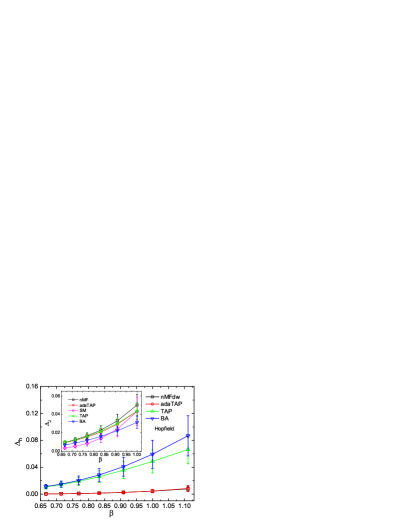
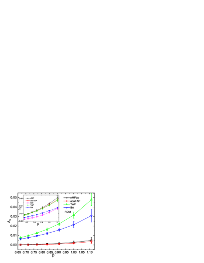
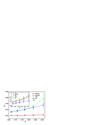
Figure 1: (Color online) Inference performances of adaTAP on Hopfield, random orthogonal and SK models with Gaussian distributed random fields, compared with those obtained by other existing mean-field methods. Magnetizations and correlations used to infer fields and couplings are calculated through exact exhaustive enumeration on networks of size $N=15$. Each data marker is the average over $20$ random realizations for which $\sigma_{h}^{2}=0.01$. (a) Results for the Hopfield model with $P=3$. (b) Results for ROM with $\alpha=0.6$. (c) Results for the SK model.

To collect the data of magnetizations and correlations, we use the exact enumeration on small-size systems of $N=15$, which produces noise-free data for predicting the underlying parameters. In this case, $M=2^{N}$. Inference results of adaTAP on these three tested models are compared with those obtained by other mean-field methods. For comparison, we briefly describe the other four existing mean-field methods for the inverse Ising problem. The couplings between spin $i$ and $j$ ($i\neq j$) are inferred as follows:

$$J_{ij}^{{\rm nMF}} =-(\mathbf{C^{-1}})_{ij},$$ (11a)

$$J_{ij}^{{\rm TAP}} =\frac{2(\mathbf{C^{-1}})_{ij}}{-1-\sqrt{1-8m_{i}m_{j}(\mathbf{C^{-1}})_{ij}}},$$ (11b)

$$J_{ij}^{{\rm SM}} =J_{ij}^{{\rm nMF}}+J_{ij}^{{\rm ind}}-\frac{C_{ij}}{L_{i}L_{j}-C_{ij}^{2}},$$ (11c)

$$J^{{\rm BA}}_{ij} =-\tanh^{-1}\Biggl{[}\frac{1}{2(\mathbf{C}^{-1})_{ij}}(a_{ij}-b_{ij})-m_{i}m_{j}\Biggr{]},$$ (11d)

where $J_{ij}^{{\rm ind}}=\frac{1}{4}\ln\left[\frac{(1+\tilde{C}_{ij})^{2}-(m_{i}+m_{j})^{2}}{(1-\tilde{C}_{ij})^{2}-(m_{i}-m_{j})^{2}}\right]$, $a_{ij}=\sqrt{1+4L_{i}L_{j}(\mathbf{C}^{-1})_{ij}^{2}}$, $b_{ij}=\sqrt{\left(a_{ij}-2m_{i}m_{j}(\mathbf{C}^{-1})_{ij}\right)^{2}-4(\mathbf{C}^{-1})_{ij}^{2}}$ and $L_{i}=1-m_{i}^{2}$. After couplings are inferred, fields can be predicted using the following equations:

$$h_{i}^{{\rm nMF}} =\tanh^{-1}(m_{i})-\sum_{j\neq i}J^{{\rm nMF}}_{ij}m_{j},$$ (12a)

$$h_{i}^{{\rm TAP}} =\tanh^{-1}(m_{i})-\sum_{j\neq i}J^{{\rm TAP}}_{ij}m_{j}$$

$$+m_{i}\sum_{j\neq i}(J^{{\rm TAP}}_{ij})^{2}(1-m_{j}^{2}),$$ (12b)

$$h_{i}^{{\rm BA}} =\tanh^{-1}(m_{i})-\sum_{j\neq i}\tanh^{-1}\left(t_{ij}f(m_{j},m_{i},t_{ij})\right),$$ (12c)

where $t_{ij}=\tanh J^{{\rm BA}}_{ij}$ and $f(x,y,t)=\frac{1-t^{2}-\sqrt{(1-t^{2})^{2}-4t(x-yt)(y-xt)}}{2t(y-xt)}$. Since SM expansion has large inference errors for predicting fields even when considering up to the third order in the small correlation expansion Sessak and Monasson (2009), we would not show its field inference performances for the temperature range we consider.

We first examine the inference performance of adaTAP on mean-field models, where quenched random fields are drawn independently at random from a Gaussian distribution with zero mean and variance $\sigma_{h}^{2}$. As displayed in Fig. 1 (a) for the Hopfield model, adaTAP shows slightly better performance than the TAP approach in coupling constructions, whereas the SM expansion has the best performance at high temperatures and the BA has the best one at low temperatures. Regarding field inference, adaTAP performs much better than other methods in the entire temperature range under consideration. However, if we incorporate an effective self-coupling (diagonal weight) $J_{ii}=\frac{1}{1-m_{i}^{2}}-(\mathbf{C^{-1}})_{ii}$ Kappen and Rodriguez (1998) into the inference equation (12a), nMF with diagonal weights (nMFdw) will achieve the nearly same accuracy with adaTAP in predicting external fields, although adaTAP still gives a bit lower inference error. This also holds for the other two mean-field models. Note that nMF without diagonal weights definitely gives a highest inference error among all mean-field methods compared here. As the temperature becomes sufficiently low, adaTAP ceases to converge within $t_{{\rm max}}$ or $t^{\prime}_{{\rm max}}$, thus becoming unable to predict couplings and fields. To infer a model with quenched random fields, TAP and BA will also have no solution at low enough temperatures. We also performed simulations with a larger $\sigma_{h}^{2}$ (e.g., $\sigma_{h}^{2}=0.1$), and it is observed that the field inference performance deteriorates and adaTAP fails to converge at a higher temperature for some samples compared to the case with a smaller field variance. Fig. 1 (b) shows inference results for ROM with the random orthogonal coupling matrix. Although adaTAP behaves slightly worse than TAP for inferring couplings, it produces surprisingly accurate estimates of external fields in the entire temperature range in Fig. 1 (b). Note that the inference accuracy obtained by other mean-field methods (except nMFdw) can be further improved by at least one order of magnitude by using adaTAP when the random fields are Gaussian distributed. For coupling inferences of the SK model (see Fig. 1 (c)), the performance of adaTAP lies between those of nMF and TAP, while the SM expansion gives a more accurate prediction than other methods at high temperatures.

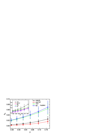
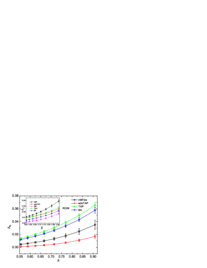
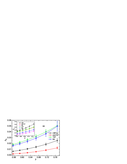
Figure 2: (Color online) Inference performances of adaTAP on Hopfield, random orthogonal and SK models with bimodal distributed random fields, compared with those obtained by other existing mean-field methods. Magnetizations and correlations used to infer fields and couplings are calculated through exact exhaustive enumeration on networks of size $N=15$. Each data marker is the average over $20$ random realizations for which $h_{0}=0.3,p=0.6$. (a) Results for the Hopfield model with $P=3$. (b) Results for ROM with $\alpha=0.6$. (c) Results for the SK model.

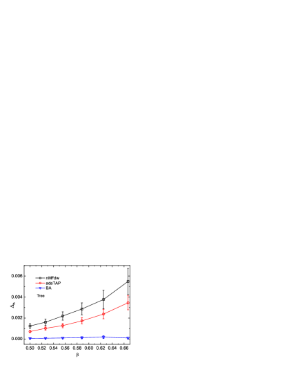
Figure 3: (Color online) Inference performances of adaTAP on a tree ($N=22$), compared with nMFdw and BA (exact method on a tree model). Each data marker is the average over $10$ random realizations.

Fortunately, the superiority of adaTAP for field inference is also true when the random field is bimodal distributed, i.e., $p_{h}(h)=p\delta(h-h_{0})+(1-p)\delta(h+h_{0})$. Its performance is shown in Fig. 2 with $p=0.6,h_{0}=0.3$. The improvement of the field prediction by adaTAP is evident in this case, even compared to nMFdw. In adaTAP, we still assume zero diagonal couplings, however, the third term inside the square bracket of Eq. (6) provides an adaptive Onsager correction to the nMF approximation, playing the same key role with diagonal couplings in inferring external fields. In this adaptive manner, lower inference error of fields and couplings is achieved compared to nMFdw. Interestingly, adaTAP can even perform better than TAP in predicting couplings for certain ranges of temperatures in this case.

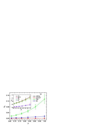
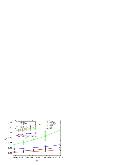
Figure 4: (Color online) Inference performances of adaTAP on diluted SK model ($p_{d}=0.4$), compared with those obtained by other existing mean-field methods. Magnetizations and correlations used to infer fields and couplings are calculated through exact exhaustive enumeration on networks of size $N=15$. Each data marker is the average over $20$ random realizations. (a) Results for the Gaussian distributed random fields with $\sigma_{h}^{2}=0.01$. (b) Results for the bimodal distributed random fields with $h_{0}=0.3,p=0.6$.

All the models investigated so far are of the fully connected type. For examining the capability to deal with another extreme of sparsely connected networks, the proposed scheme is also tested on a tree model. Our proposed scheme performs better than other methods except BA which is exact on a tree and gives very accurate inference both on the couplings and fields. The result is shown in Fig. 3. A tree of size $N=22$ is constructed, such that each node inside the tree has degree equal to $3$, and to mimic an infinite Bethe lattice, we generate the external fields for the boundary spins as $\hat{h}_{i}=h_{i}+\sum_{k\in\partial i\backslash j}h_{k\rightarrow i}$, where $j$ is the only spin inside the tree connected to the boundary spin $i$ and the cavity field $h_{k\rightarrow i}$ is randomly chosen from a population dynamics for an infinite Bethe lattice Mézard and Parisi (2001). Couplings and fields ($h_{i}$ for the boundary spins) for the tree follow Gaussian distributions $\mathcal{N}(0,1)$ and $\mathcal{N}(0,0.01)$ respectively. Magnetizations and correlations are calculated by using susceptibility propagation algorithms Huang and Zhou (2012). However, in real applications, for example, a typical neuronal network of size around $N=100$ is not strongly diluted with an exact tree structure, therefore, our method is expected to still give good estimates of external fields. To confirm this point, we test adaTAP on a diluted SK model, where each non-zero Gaussian distributed coupling is present with a predefined probability $p_{d}$. The Gaussian distribution has zero mean and variance $1/c$ with $c=p_{d}N$. As shown in Fig. 4, the adaTAP still performs better than other mean-field methods (including nMFdw) in field inference, which is much more evident when random fields are bimodal distributed.

Although adaTAP, TAP, and the BA will have no solution in inferring mean-field models with quenched random fields at low temperatures, adaTAP does outperform other existing mean-field methods compared here to infer quenched random fields if it converges, as shown for a wide range of temperatures on the Hopfield, random orthogonal and (diluted) SK models. We conclude that the power of adaTAP for inverse Ising problems resides in its remarkable accuracy in predicting external fields, especially for the case where there is a single dominant state in phase space.

IV Conclusion

In summary, we propose the adaTAP approach for inverse Ising problems and show its striking performance for inferring external fields in mean-field models. As far as the field inference is concerned, adaTAP is rather satisfactory, compared to other mean-field methods. Furthermore, an accurate inference of external fields in the Ising model is able to provide us with insights into the mechanism underlying high-throughput data either coming from biological experiments or from large databases Schneidman et al. (2006); Weigt et al. (2009); Marks et al. (2011). The proposed adaTAP approach for the inverse Ising problem is expected to have applications in real data analyses (e.g., neural data, or sequences in the protein databases), in combination with other mean-field methods.