Experimental quantum Zeno effect in NMR with entanglement-based measurement

Abstract

We experimentally demonstrate a new dynamic fashion of quantum Zeno effect in nuclear magnetic resonance systems. The frequent measurements are implemented through quantum entanglement between the target qubit(s) and the measuring qubit, which dynamically results from the unitary evolution of duration $\tau_{m}$ due to dispersive-coupling. Experimental results testify the presence of “the critical measurement time effect”, that is, the quantum Zeno effect does not occur when $\tau_{m}$ takes the some critical values, even if the measurements are frequent enough. Moreover, we provide a first experimental demonstration of an entanglement preservation mechanism based on such dynamic quantum Zeno effect.

I Introduction

The quantum Zeno effect (QZE) describes the situation of the inhibition of transitions between quantum states by frequent measurements Sudarshan1977 . As observed in some experiments, e.g., using trapped ion Wineland1990 , cold atoms Raizen2001 , cavity quantum electrodynamics Bernu2008 , nuclear magnetic resonance (NMR) Li2006 , QZE was often regarded as the experimental witness of projection measurement, or called the wave-packet collapse (WPC), since the first interpretation of QZE was made according to WPC. However, many people questioned this opinion by re-explaining these experimental observations with some dynamic fashions without invoking WPC Schenzle1991 . In the approach of Ref.Xu2011 , each measurement is implemented as a dynamical unitary evolution driven by a dispersive-coupling of the measured system to the apparatus with duration $\tau_{m}$. Actually, the free evolution causes the deviation of the system from its initial state, while the dynamic measurements can interrupt the evolution by adding a phase factor to the resulting state of the system, leading to QZE. However, the dynamical phase effect depends on the measurement time $\tau_{m}$. When $\tau_{m}$ takes some critical values $\tau_{m}^{\ast}$, each dynamical phase factor in the measurements corresponding to some integer phase in units of ${\rm{2}}\pi$, the system is unaffected by the measurements. In this case, no QZE occurs. We call this phenomenon the critical measurement time effect Xu2011 .

In this paper, we experimentally reveal this $\tau_{m}$-dependence in a NMR ensemble when the measurements are treated by unitary dynamical processes. We first carried out experiments with one single-qubit system and one measuring qubit. Besides the effects predicted by the conventional QZE, the role of critical $\tau_{m}^{\ast}$ is also clearly demonstrated in the experiments. From the view of the experiment, the dynamic measurement model is more compatible with the physical reality in comparison with the projection measurement in respect of the QZE. Therefore it can be regarded as an active mechanism protecting the system from deviating from its initial state. We also experimentally implement such a scheme of entangled-state-preservation in a two-qubit system via QZE, which is significant to quantum information and computation.

II a dynamic approach for QZE and the critical measurement time effect

A general dynamic approach for QZE is described with a sequence of $N$ frequent measurements inserted in a unitary free evolution described by $U\left(\tau\right)$, as illustrated in Fig.1(a). Each measurement is of duration $\tau_{m}$ with equal time intervals $\tau+\tau_{m}$, and is also described by a unitary operator $M=M\left(\tau_{m}\right)=e^{-iH_{M}\tau_{m}}:\left|s_{j}\right\rangle\otimes\left|a\right\rangle\rightarrow\left|s_{j}\right\rangle\otimes\left|a_{j}\right\rangle.$ The corresponding Hamiltonian $H_{M}=H_{S}+H_{A}+H_{int}$ describes the time evolution of a closed system formed by the measured system $S$ plus the apparatus $A$ with the Hamiltonian $H_{S}$ and $H_{A}$, correspondingly. $M$ dynamically results in an entanglement between $S$ and $A$ with the initial state $\left|a\right\rangle$. Here, $\left|s_{j}\right\rangle$ are the orthonormal states of $S$, but the states $\left|a_{j}\right\rangle$ of $A$ need not to be orthonormal with each other. The entanglement-based measurement means that one could readout the system state $\left|s_{j}\right\rangle$ from the apparatus state $\left|a_{j}\right\rangle$. Such measurement $M$ is realized by the dispersive coupling $H_{int}$ of $A$ to $S$, which is so strong that we do not consider the relatively weak free evolution during measurements. Usually we chose $\left|s_{j}\right\rangle$ to be the eigenstate of the system Hamiltonian $H_{S}$, which satisfies $\left[H_{S},H_{int}\right]=0$, thus $M$ obviously represents a quantum nondemolition (QND) measurement Braginsky1996 .

As illustrated in Fig.1(a), the total time evolution describing the QZE reads as $U_{tot}\left(t\right)=\left[M\left(\tau_{m}\right)U\left(\tau\right)\right]^{N}$ with the total free evolution time $t=N\tau$ fixed. In the limit $\tau\rightarrow 0$ and meanwhile $t$ keeps constant, $U_{tot}\left(t\right)$ becomes diagonal with respect to $\left|s_{j}\right\rangle$, thus such evolution process due to dispersive-coupling inhibits the transitions among the states $\left|s_{j}\right\rangle$. Remarkably, $U_{tot}\left(t\right)$ is not always diagonal for arbitrary $\tau_{m}$ even in the limit $\tau\rightarrow 0$. When $\tau_{m}$ is accessing certain critical values $\tau_{m}^{\ast}=2\pi n/\Delta,\,n=0,1,2,\dots,$ the system exhibits no QZE, where $\Delta$ roughly represents the energy level spacing of the system, and thus the precise form of $\tau_{m}^{\ast}$ depends on the concrete model.

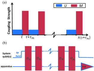
Figure 1: (color online). (a) General dynamic approach for QZE and (b) the corresponding schematic diagram for experiments. Frequent measurements $M$ are driven by the interaction Hamiltonian $H_{M}$, while the free evolution $U$ of the system are implemented by RF pulses applied on the system. In the end, we read out the information about the system just from the apparatus via QND measurement. The free-evolution $U$-process is neglected during strong measurement $M$-process.

Figure 1(b) shows the corresponding schematic diagram for the experiment to demonstrate the above entanglement-based QZE in a NMR spin system. The system consists of nuclear spins $I_{j}(j=1,2,...n)$, while the apparatus is nuclear spin $I_{0}$, called the measuring qubit. In a static longitudinal magnetic field, the ($n$+1)-spin system has the natural Hamiltonian

$$H_{nmr}=2\pi\sum\limits_{j=0}^{n}{\upsilon_{j}}I_{z}^{j}+2\pi\sum\limits_{j<k,=0}^{n}{J_{jk}}I_{z}^{j}I_{z}^{k},$$ (1)

where $\upsilon_{j}$ is Larmor frequency of spin $j$ and $J_{jk}$ is the scalar coupling strength between spins $j$ and $k$. The free evolution of the system is implemented by radio frequency (RF) pulses, and in multiply rotating frame $U\left(\tau\right)=e^{-iH_{free}\tau}$ is then driven by the Hamiltonian

$$H_{free}=2\pi\sum\limits_{j=1}^{n}({\delta_{j}I_{z}^{j}+P_{j}I_{x}^{j}}).$$ (2)

Here the chemical shifts $\delta_{j}=\upsilon_{j}-\Omega_{j}$ and we assume the individual nuclear spin $I_{j}$ can be independently excited with frequency $\Omega_{j}$ (e.g. hereto-nuclear NMR systems) and the strength $P_{j}$ of the RF field is so large that the spin-spin couplings of strength $J_{ij}$ could be ignored when the RF fields are applied to the system (usually the hard RF pulses have this property $P_{j}\gg|J_{ij}|$). A sequence of RF pulses with frequencies $\Omega_{j}$ are periodically applied to the system. Between the RF pulses, the spin-spin couplings are employed to implement an entanglement-based measurement $M=M\left(\tau_{m}\right)$ through a measurement Hamiltonian $H_{M}$:

$$H_{M}=H_{S}+2\pi\sum\limits_{j=1}^{n}{J_{0j}}I_{z}^{0}I_{z}^{j}.$$ (3)

Here, we have chosen $H_{A}$ = 0 (i.e., $\delta_{0}=0$), and $H_{int}=2\pi\sum\limits_{j=1}^{n}{J_{0j}}I_{z}^{0}I_{z}^{j}$. Due to the fact $P_{j}\gg|J_{ij}|$, the role of $U(\tau)$ in the total time evolution is dominated with respect to $M$ in our experiment, which is just opposite to the scheme illustrated in Fig. 1(a). However, this does not influence our result as we only require the $U$ and $M$ processes can be well separated in time domain. In order to observe the dynamic QZE with the QND measurement, we require to prepare the initial state $|s\rangle$ of the system into an eigenstate of $H_{S}$.

To ascertain whether the system deviates from its initial state at the end of time evolution, we need to read out the information about the system through a QND measurement on the measuring qubit. The interaction Hamiltonian $H_{int}$ in $H_{M}$ is chosen to satisfy $\left[H_{int},H_{S}\right]=0$, thus $M$ represents a QND measurement. Furthermore, $\left[H_{A},H_{int}\right]=0$ guarantees a measurement scheme analogy to the Ramsey interference, which can be used in our experiments to detect the deviation of the final state from its initial state. To this end, the apparatus $I_{0}$ is prepared in a superposition state $\left|a\right\rangle=\left(\left|0\right\rangle+\left|1\right\rangle\right)/\sqrt{2}$. Then $U_{tot}\left(t\right)$ will evolve the initial product state $\left|\varphi\left(0\right)\right\rangle=\left|s\right\rangle\otimes\left|a\right\rangle$ to a quantum entanglement $\left|\varphi\left(t\right)\right\rangle=\frac{1}{\sqrt{2}}(U_{-}\left|s\right\rangle\left|0\right\rangle+U_{+}\left|s\right\rangle\left|1\right\rangle)$, where $U_{-}\left(t\right)=\langle 0|U_{tot}\left(t\right)\left|0\right\rangle$ and $U_{+}\left(t\right)=\langle 1|U_{tot}\left(t\right)\left|1\right\rangle$. $U_{\pm}\left(t\right)$ has the similar limitation behavior $\lim_{N\rightarrow\infty}\left|U_{\pm}\left(t\right)\right|\rightarrow 1$ as $U_{tot}\left(t\right)$, thus the system is frozen in its initial state by the frequent measurements. Consequently, we can obtain the state information of the system by measuring the magnitude of the conherence of spin $I_{0}$, i.e., the off-diagonal element of its reduced density matrix:

$$\mathcal{D}=\left|\left\langle s\right|U_{+}^{\dagger}\left(t\right)U_{-}\left(t\right)\left|s\right\rangle\right|.$$ (4)

When the QZE occurs, $U_{\pm}\left(t\right)$ freezes the initial state $\left|s\right\rangle$ up to a change of the phase factor, thus $\mathcal{D}$ equals to unity. However, when $U_{\pm}\left(t\right)$ evolves the system away from its initial state, then $\mathcal{D}$ should present an oscillating dynamics. Accordingly, the behavior of $\mathcal{D}$ provides us the information of whether the QZE happens. Additionally, the experimental values of $\cal D$ can relatively easily be obtained, thanks to the quadrature detecting technology in NMR signal detection.

III Experiment

The experiment was realized at room temperature on a Bruker AV- 400 spectrometer ($B_{0}=9.4T$) . The physical system we used is the ${}^{13}C$-labeled Diethyl-fluoromalonate dissolved in ${}^{2}H$-labeled chloroform Lu2011 , where ${}^{13}C$ is chosen as the measuring qubit $I_{0}$, and ${}^{19}F$ and ${}^{1}H$ as the system qubits $I_{1}$ and $I_{2}$, respectively. The J-coupling constants $J_{12}=48.3$ Hz, $J_{02}=160.7$ Hz and $J_{01}=-194.4$ Hz. We first initialized the system in a pseudopure state (PPS) $\rho_{000}=(1-\epsilon)\mathbf{1}/8+\epsilon\left|000\right\rangle\left\langle 000\right|$ using the spatial average technique Cory1997 , where $\mathbf{1}$ representing the $8\times 8$ identity operator and $\epsilon\approx 10^{-5}$ the polarization. Then the measuring qubit (${}^{13}C$) was prepared into the superposition state $\left|a\right\rangle=\left(\left|0\right\rangle+\left|1\right\rangle\right)/\sqrt{2}$ by a $\pi/2$ pulse along $y$ axis. In order to observe the dynamic QZE in different quantum systems, i.e, a single-qubit system and a composite two-qubit system, we performed two sets of the experiments. Figure. 2 shows the experimental pulse sequences for observing the entanglement-based QZE in the single-qubit system and the composite two-qubit system.

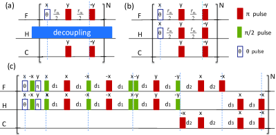
Figure 2: (color online). Pulse sequences for observing entanglement-based QZE: in a single-qubit system (a), and in a composite system for a product state $|00\rangle$ (b) and for a pseudo-entangled state $\left|\phi^{+}\right\rangle$ (c). Each M-process lasts about $2.5\sim 3.0ms$ for the single-qubit system and about $28\sim 33ms$ for the composite system. Here, $\theta{\rm{=}}{5^{\circ}}\sim{6^{\circ}}$, $\eta=400\pi{\tau_{m}}$, ${d_{1}}=\frac{{100{\tau_{m}}}}{{2\left|{{J_{12}}}\right|}}$, ${d_{2}}=\frac{{250{\tau_{m}}}}{{2\left|{{J_{01}}}\right|}}$ and ${d_{3}}=\frac{{250{\tau_{m}}}}{{2\left|{{J_{02}}}\right|}}$.

To observe QZE in a single-qubit system, we took only spin $I_{1}$ as the system while decoupling spin $I_{2}$ during the whole experiment. The initial state of spin $I_{1}$, $|s\rangle=|0\rangle$, and the natural Hamiltonian $H_{nmr}$ in Eq. (1) can be the measurement Hamiltonian $H_{M}$, i.e., $H_{M}=2\pi\delta_{1}I_{z}^{1}+2\pi J_{01}I_{z}^{0}I_{z}^{1}$. We can obtain the critical measurement time $\tau_{m}^{\ast}=n/(\delta_{1}+J_{01}m_{0})$ ($n=0,1,2,\dots$) for this case. In the experiment, we set $\delta_{1}=300Hz$, the strength of the RF field $P_{1}=18000Hz\gg J_{01}$ and the duration of these RF pulses $\tau=1\mu s$. A series of RF pulses and measurements were performed on the system for the different measurement times. We measured the NMR signal intensity of ${}^{13}C$ as a function of the pulse number $N$, which is directly proportional to the coherence $\mathcal{D}$ of spin $I_{0}$. Figure 3(a) shows the experimental data for the measurement time at the critical value $\tau_{m}=\tau_{m}^{\ast}=2.517ms$ (denoted by the dots), at $\tau_{m}=2.55ms$ nearby the critical value (denoted by the triangles) and at $\tau_{m}=3ms$ far from the critical value (denoted by the squares), along with the theoretical expectations (denoted by the solid lines) obtained by numerical simulations. As expected, when the measurement time $\tau_{m}$ is set at the critical value $\tau_{m}^{\ast}$, NMR signal intensity presents a Rabi oscillation; when $\tau_{m}$ is far from $\tau_{m}^{\ast}$, the usual QZE occurs where the frequent measurements would largely inhibit the unstable system from evolving to other states; when $\tau_{m}$ is close to $\tau_{m}^{\ast}$, we observe the deviation from usual QZE and $\mathcal{D}$ shows a suppressed oscillation. This $\tau_{m}$-dependent entanglement-based QZE now is shown in our NMR experiment.

Meanwhile, we observed the decay of the NMR signals in Fig.3(b) (left side). This is mainly caused from the relaxation and the RF inhomogeneity. The transverse relaxation time $T_{2}^{*}$ are respectively about 300ms for ${}^{13}C$ and 800ms for ${}^{19}F$, while each M-process lasts about $2.4\sim 3ms$ (Fig.2). In order to improve experimental precision and get a better observation of our phenomenon, we engineered the unitary operation $[M(\tau_{m})U(\tau)]^{k}$ of the $k$ cycles as a single shaped pulse by the gradient ascent pulse engineering (GRAPE) algorithm Khaneja2005 , where $k$ ranges from 1 to $N$. All these GRAPE pulses are of the duration around $2.5ms$ with the theoretical fidelity above 0.99. Thus the decay caused by relaxation can be almost neglected. We can see the deviation is maximize when $\tau_{m}$ reaches to $\tau_{m}^{\ast}$, ranging almost from 0 to 1. These pulses are also designed to be robust against the RF inhomogeneity. The GRAPE-based results shown in Fig. 3(b) (right side) give good description of the entanglement-measurement QZE.

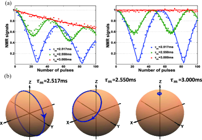
Figure 3: (color online). Experimental QZE with entanglement-based measurement on single qubit system. (a) Experimental observations of QZE with a series of RF pulses and measurements (left side) and with GRAPE engineering (right side). The amplitude decay in the left pannel is simulated by adding an exponential decay $\exp\left(-k\tau_{m}\right)$ to each $M$-process ($k=1.25$, $0.8$ and $0.7$, respectively, for $\tau_{m}=2.517ms,2.55ms$ and $3ms$). (b) Evolution paths of the system on the Bloch sphere, corresponding to the three experiments with the measurement times $\tau_{m}=2.517ms,2.550ms,3.000ms$.

In the second set of the experiment, we further demonstrate entanglement-based QZE in a composite system consisting of spins $I_{1}$ and $I_{2}$. Here, we considered two different initial states of the system: the product PPS $|00\rangle$ and the pseudo-entangled state $\left|\phi^{+}\right\rangle=\left(\left|01\right\rangle+\left|10\right\rangle\right)/\sqrt{2}$ pps_notes obtained from $|00\rangle$ by NOT gate, Hadamard gate and CNOT gate. Therefore, two kinds of spin-spin couplings are involved in the measurement Hamiltonians for QND measurements. For the product state, $H_{M}=2\pi\sum\limits_{j=1}^{2}{\delta_{j}}I_{z}^{j}+2\pi\sum\limits_{j<k,=0}^{2}{J_{jk}}I_{z}^{j}I_{z}^{k}$ (i.e., the natural Hamiltonian of these three-spin NMR system in the multiply rotating frame). In this case, the critical measurement time can be obtained as $\tau_{m(PPS)}^{\ast}=n/\left(\eta_{j}+J_{12}/2\right)$ for $j=1,2$, $n=0,1,2,\dots$, where $\eta_{j}=\delta_{j}\pm J_{0j}/2$. We set $\delta_{1}=\delta_{2}=400$ in the experiment. For the entangled state, $H_{M}=2\pi\sum\limits_{j=1}^{2}{\delta_{j}}I_{z}^{j}+2\pi\mathcal{J}_{12}\mathbf{I}^{1}\cdot\mathbf{I}^{2}+2\pi\sum\limits_{j=1}^{2}{\mathcal{J}_{0j}I_{z}^{0}I_{z}^{j}}$, where $H_{S}=2\pi\sum\limits_{j=1}^{2}{\delta_{j}}I_{z}^{j}+2\pi\mathcal{J}_{12}\mathbf{I}^{1}\cdot\mathbf{I}^{2}$, which is Heisenberg-XXX-coupling (or isotropic Heisenberg) type. Similarly, $\tau_{m(ENT)}^{\ast}=n/(\delta_{j}\pm\mathcal{J}_{0j}/2)$. It is easy to find that $\left|\phi^{+}\right\rangle$ is a non-degenerate eigenstate of $H_{S}$, and $[H_{S},H_{int}]=0$ when $\delta_{1}=\delta_{2}$ and $\mathcal{J}_{01}=\mathcal{J}_{02}$. In experiment, $\delta_{1}=\delta_{2}=200$, $\mathcal{J}_{12}=100$, and $\mathcal{J}_{01}=\mathcal{J}_{02}=250$. Note that $\mathcal{J}_{ij}$ are not the same as ones in the nature Hamiltonian $H_{nmr}$. Consequently, we can experimentally achieve the evolution of $H_{M}$ by quantum simulation technique peng05 .

However, the direct simulation of the Hamiltonian $H_{M}$ requires a long operation time to realize the measurement $M(\tau_{m})$, especially in the case of the entangled state (about $26\sim 31ms$) (Fig.2). Relaxation will be a serious problem. Accordingly, we adopted the GRAPE engineering here for precise quantum control. The experimental results are shown in Fig. 4, which illustrates the $\tau_{m}$-dependent behavior in entanglement-based QZE both for the product state and the entangled state, like the single-qubit system. At the critical measurement time $\tau_{m}^{*}$ e.g., $\tau_{m(PPS)}^{*}=3.059ms$ and $\tau_{m(ENT)}^{*}=3.077ms$, $\mathcal{D}$ oscillates almost from 0 to 1. When $\tau{}_{m}$ is right around $\tau_{m}^{*}$, e.g., $\tau_{m(PPS)}=3.1ms$ and $\tau_{m(ENT)}=3.2ms$, we can see the amplitude of oscillations of $\mathcal{D}$ decays quickly. $\mathcal{D}$ has almost no change at $\tau_{m(PPS)}=3.5ms$, $\tau_{m(ENT)}=3.7ms$, representing the QZE occurs and the preservation of quantum states works well. To assess the quality of the QZE, we also carried out full quantum state tomography for the initial state and the final state after N pulses for the case of the entangled state, shown in Fig. 4(c). With the help of the GRAPE pulses, we have successfully preserved the entangled state with a high fidelity running up to 0.99 State_F .

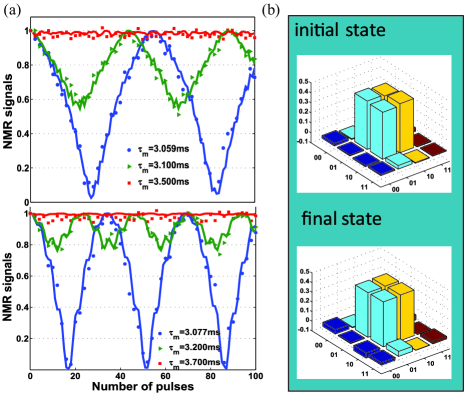
Figure 4: (color online). (a) Experimental QZE with entanglement-based measurement on two-qubit system for a product state (top plots) and (b) an entangled state (bottom plots). (b) Real part of the reconstructed density matrix of the initial and final state for preserving the entangled state via QZE.

IV further discussion

In the end, we further analyze the dynamic theory of QZE to explain the experimental results. For the single-qubit system, the first free evolution of $U\left(\tau\right)$ evolves the initial state $|s\rangle=|0\rangle$ to a superposition state: $U\left(\tau\right)|0\rangle=a|0\rangle+b|1\rangle$. Then, it undergoes a measurement process $M(\tau_{m})$ to $|\psi_{1}\rangle=M(\tau_{m})U\left(\tau\right)|0\rangle=e^{-i\pi(\delta_{1}+J_{01}m_{0})\tau_{m}}a|0\rangle+e^{i\pi(\delta_{1}+J_{01}m_{0})\tau_{m}}b|1\rangle$ with $m_{0}=\pm 1/2$ depending on a state of spin $I_{0}$, $|0\rangle$ or $|1\rangle$. The measurement adds a phase shift between $|0\rangle$ or $|1\rangle$ of the system state: $\Delta\phi=2\pi(\delta_{1}+J_{01}m_{0})\tau_{m}$. Therefore, we can see three different situations from the phase shift. ($i$) When $\tau_{m}=\tau_{m}^{\ast}=n/(\delta_{1}+J_{01}m_{0})$ ($n=0,1,2,\dots$), the phase shift $\Delta\phi=2n\pi$ and $|\psi_{1}\rangle=e^{-in\pi}\left(a|0\rangle+b|1\rangle\right)$. This implies that the measurement with the critical time only gives a whole phase factor $e^{-in\pi}$ to the state. The repeated applications of the pulse and measurement drive the system to undergo a Rabi oscillation like the behavior of a continuous RF pulse except for a whole phase factor, and no QZE occurs. ($ii$) When $\tau_{m}=(n-1/2)/(\delta_{1}+J_{01}m_{0})$, the phase shift $\Delta\phi=(2n-1)\pi$ and $|\psi_{1}\rangle=e^{-i(n-1/2)\pi}\left(a|0\rangle-b|1\rangle\right)$. State $|1\rangle$ acquires a phase of $-1$ with respect to $|0\rangle$ (that is, a $\pi$-phase shift). Hence, the evolution of the system spin is reversed after each measurement is applied, thus reversing the free evolution of the system and QZE occurs. This has a similar behavior to “bang-bang control” Facchi2004 ; morton2005 . It is not necessary to apply perfect $\pi$-phase shifts to lock the spin. ($iii$) When the measurement time has a small deviation $\xi$ from $\tau_{m}^{\ast}$, i.e., $\tau_{m}=\tau_{m}^{\ast}+\xi$, the intermediate case occurs. We have $|\psi_{1}\rangle=e^{-i2\pi(\delta_{1}+J_{01}m_{0})I_{z}^{1}\tau_{m}}e^{-i2\pi(\delta_{1}I_{z}^{1}+P_{1}I_{x}^{1})\tau}|0\rangle\approx e^{-i2n\pi I_{z}^{1}}e^{-i2\pi\left\{[(\delta_{1}+J_{01}m_{0})\xi/\tau+\delta_{1}]I_{z}^{1}-i2\pi P_{1}I_{x}^{1}\right\}\tau}|0\rangle$. This functions as a RF rotation around an axis in the XZ plane, and the situation is similar to the first one, only with different amplitude. In fact, this approximation always makes the whole unitary propagator $[M(\tau_{m})U(\tau)]^{N}$ for $N$ repeated cycles good in the wide range of $\xi$ in our experiment due to $\tau\to 0$. However, when $|(\delta_{1}+J_{01}m_{0})\xi|\gg P_{1}\tau$, $M(\tau_{m})U(\tau)$ is a rotation almost around the $z$ axis, which results in the initial state $|0\rangle$ unchanged. When $|\xi|$ reaches $0.5/|\delta_{1}+J_{01}m_{0}|$, we exactly return to the situation ($ii$). Consequently, the intermediate phenomenon occurs only in a range of $|(\delta_{1}+J_{01}m_{0})\xi|\sim P_{1}\tau$, where $P_{1}\tau\approx 0.018$ in the experiment. Figure 3(b) shows clearly the corresponding evolutions of the system qubit on the Bloch sphere for these three situations. The similar analysis can be also used to explain the experiments on the two-qubit composite system.

V CONCLUSIONS

In conclusion, we have experimentally demonstrated the QZE with entanglement-based measurement in a NMR ensemble, where the frequent measurements are implemented through the dispersive-coupling between the target system and the measuring qubit. Therefore, the measurement is dynamically described by the unitary evolution of duration $\tau_{m}$, rather than the projection measurements. With a three-qubit NMR system, we have successfully observed the dynamic QZE of a single-qubit system as well as the composite system, especially an entanglement preservation. Our experiment also clearly shows the dependence of this dynamic QZE on the measurement time $\tau_{m}$ in the frequent measurements: the system exhibits no QZE at certain critical measurement times $\tau_{m}^{\ast}$. This well distinguishes from the usual one based on projection measurements. Moreover, we have experimentally demonstrated nontrivial quantum-state steering towards the efficient preservation of entanglement using the dynamical QZE.

Appendix A critical measurement times

Now we analyze the critical measurement times for two typical cases in the experiments: the single-qubit system and the composite system. In the single-qubit system, the free evolution Hamiltonian is $H_{free}=2\pi(\delta_{1}I_{z}^{1}+P_{1}I_{x}^{1})$ and the measurement Hamiltonian $H_{M}=2\pi(\delta_{1}I_{z}^{1}+J_{01}I_{z}^{0}I_{z}^{1})$. Following the same procedure in Ref.$\left[7\right]$, the total time evolution operator is determined as

$$U_{tot}\left(t\right) \approx \exp\left[-2\pi i\delta_{1}I_{z}^{1}t+\frac{P_{1}\tau}{2}\left(f_{1}+h.c.\right)\right]M\left(N\tau_{m}\right).$$

Here, we neglect the high order terms of $\tau$ in the exponent and denote that

$$f_{1} = I_{+}^{1}e^{-i\pi\left(N+1\right)\tau_{m}\left(\delta_{1}+J_{01}I_{z}^{0}\right)}\frac{\sin\left[\pi N\tau_{m}\left(\delta_{1}+J_{01}I_{z}^{0}\right)\right]}{\sin\left[\pi\tau_{m}\left(\delta_{1}+J_{01}I_{z}^{0}\right)\right]},$$

where $I_{+}^{1}=I_{x}^{1}+iI_{y}^{1}$. When the measurement time approaches to the critical value $\tau_{m}^{\ast}=n/\left(\delta_{1}+J_{01}m_{0}\right)$, ($n=0,1,2,\dots$, and $m_{0}=+1/2$ or $-1/2$, the eigenvalue of $I_{z}^{0}$ according to its the initial state), $f_{1}$ is proportional to $NI_{+}^{1}$, thus $U_{tot}\left(t\right)\sim\exp\left[-2\pi i(\delta_{1}I_{z}^{1}+P_{1}I_{x}^{1})t\right]$ will drive the system oscillating and the QZE is violated. Otherwise, when the measurement time is not around $\tau_{m}^{\ast}$, $f_{1}$ is finite hence $U_{tot}\left(t\right)$ becomes a unit operator in the limit $\tau\rightarrow 0$.

For the product state $\left|00\right\rangle$ of the composite system, the measurement Hamiltonian with Ising-type coupling is $H_{M}=2\pi\sum\limits_{j=1}^{2}{\delta_{j}}I_{z}^{j}+2\pi\sum\limits_{j<k,=0}^{2}{J_{jk}}I_{z}^{j}I_{z}^{k}$. We find that the total time evolution operator reads

$$\begin{array}[]{ll}&U_{tot}\left(t\right)\approx\\ &\exp\left\{-i\sum_{j=1,2}\left[2\pi\delta_{j}I_{z}^{j}t+\frac{\tau P_{j}}{2}\left(f_{j}+h.c.\right)\right]\right\}M\left(N\tau_{m}\right),\end{array}$$ (5)

where

$$f_{j} =I_{+}^{j}e^{-i\pi\left(N+1\right)\tau_{m}\left(\eta_{j}+\frac{1}{2}J_{12}\right)}\frac{\sin\left[\pi N\tau_{m}\left(\eta_{j}+\frac{1}{2}J_{12}\right)\right]}{\sin\left[\pi\tau_{m}\left(\eta_{j}+\frac{1}{2}J_{12}\right)\right]},$$

where $I_{+}^{j}=I_{x}^{j}+iI_{y}^{j}$ and $\eta_{j}=\delta_{j}+J_{0j}m_{0}$. When the measurement time approaches to the critical value $\tau_{m}^{\ast}=n/\left(\eta_{j}+J_{12}/2\right)$, ($n=0,1,2,\dots$), as the same reason in the single-qubit case, $U_{tot}\left(t\right)$ is proportional to $\exp\left[-2\pi i(\delta_{j}I_{z}^{j}+P_{j}I_{x}^{j})t\right]$, which violates the QZE. Similarly, we can obtain the critical measurement time $\tau_{m}^{\ast}=n/(\delta_{j}\pm\mathcal{J}_{0j}/2)$ for the case of the XXX coupling.

References

- (1) B. Misra and E.C.G. Sudarshan, J. Math. Phys.(N.Y.) 18, 756 (1977).
- (2) W.M. Itano, D.J. Heinzen, J.J. Bollinger, and D.J. Wineland, Phys. Rev. A 41, 2295 (1990).
- (3) M.C. Fischer, B. Gutierrez-Medina, and M.G. Raizen, Phys. Rev. Lett. 87, 040402 (2001); E.W. Streed, et al. 97, 260402 (2006).
- (4) J. Bernu et al., Phys. Rev. Lett. 101, 180402 (2008).
- (5) X. Li and A.J. Jonathan, Phys. Lett. A 359, 424-427 (2006); G.A. lvarez, D.D.B. Rao, L. Frydman, and G. Kurizki, Phys. Rev. Lett. 105, 160401 (2010).
- (6) V. Frerichs and A. Schenzle, Phys. Rev. A 44, 1962 (1991); L.S. Schulman, Phys. Rev. A 57, 1509 (1998); A. Peres, Am. J. Phys. 48, 931 (1980); L.E. Ballentine, Phys. Rev. A 43, 5165 (1991); T. Petrosky, S. Tasaki, and I. Prigogine, Phys. Lett. A 151, 109 (1990); Physica A 170, 306 (1991); S. Pascazio and M. Namiki, Phys. Rev. A 50, 4582 (1994); C.P. Sun, X.X. Yi, and X.J. Liu, Fort. Phys. 43, 585 (1995).
- (7) D.Z. Xu, Q. Ai, and C.P.Sun, Phys. Rev.A, 83, 022107(2011).
- (8) V.B. Braginsky, and F.Y. Khalili, Rev. Mod. Phys. 68, 1 (1996).
- (9) P. Facchi, D.A. Lidar, and S. Pascazio, Phys. Rev. A 69, 032314 (2004).
- (10) D.W. Lu et al., Phys. Rev. Lett. 107, 020501 (2011).
- (11) D.G. Cory, A.F. Fahmy, and T.F. Havel, Proc. Natl. Acad. Sci. U.S.A. 94, 1634 (1997).
- (12) N. Khaneja et al., J. Magn. Reson. 172, 296 (2005).
- (13) Here we omitted the unit part and only wrote down the pure-state part in PPS.
- (14) X.H. Peng, and D. Suter, Front. Phys. China 5, 1 (2010).
- (15) The state fidelity is calculated by , and represent density matrixes of the initial state and final state, respectively.
- (16) J.J.L. Morton, et al. Nature Phys. 2, 40-43 (2005).