Water Maser Survey on AKARI and IRAS Sources:
A Search for “Low-Velocity” Water Fountains

Abstract

We present the results of a 22 GHz H₂O maser survey toward a new sample of AGB and post-AGB star candidates. Most of the objects are selected for the first time based on the AKARI data, which have high flux sensitivity in the mid-infrared ranges. We aim at finding H₂O maser sources in the transient phase between the AGB and post-AGB stage of evolution, where the envelopes start to develop large deviations from spherical symmetry. The observations were carried out with the Effelsberg 100 m radio telescope. Among 204 observed objects, 63 detections (36 new) were obtained. We found 4 objects which may be “water fountain” sources (IRAS 15193$+$3132, IRAS 18056$-$1514, OH 16.3$-$3.0, and IRAS 18455$+$0448). They possess an H₂O maser velocity coverage much smaller than those in other known water fountains. However, the coverage is still larger than that of the 1612 MHz OH maser. It implies that there is an outflow with a higher velocity than the envelope expansion velocity (typically $\leq$25 km s^-1), meeting the criterion of the water fountain class. We suggest that these candidates are possibly oxygen-rich late AGB or early post-AGB stars in a stage of evolution immediately after the spherically symmetric AGB mass-loss has ceased.

1 Introduction

The circumstellar envelopes of oxygen-rich asymptotic giant branch (AGB) stars are well known emitters of OH, H₂O and SiO masers. In particular, 22 GHz H₂O masers mainly occur in the region beyond the dust formation zone. Their spectral profiles are sensitive to the mass-loss rate as well as to the geometry of the envelopes (e.g. Engels et al., 1986; Likkel et al., 1992). Thus, by observing H₂O masers we are able to study in detail the kinematics of the envelopes of evolved stars, which are usually optically opaque in short wavelengths.

Maser surveys are commonly performed by single-dish radio telescopes. However, prior to the launching of the Infrared Astronomical Satellite (IRAS), selecting suitable observing targets was not easy due to limited methods for identifying evolutionary status. The efficiency has been improved after van der Veen & Habing (1988) suggested the stellar classification method using the IRAS two-color diagram, and since then the IRAS colors have become a main criterion used in source selection for many maser surveys. The color used is defined as $[m]$$-$$[n]$=$2.5\log(F_{n}/F_{m})$, where $F_{m}$ and $F_{n}$ represent the fluxes at $m$ and $n$ $\mu$m bands, respectively. The H₂O maser survey reported by Engels & Lewis (1996) was a notable early example using the IRAS Point Source Catalog. The authors selected over 300 OH/IR stars, which are oxygen-rich late AGB stars with very thick envelopes, based on their IRAS [12]$-$[25] and [25]$-$[60] colors. They achieved a detection rate up to $\sim$50% using the Effelsberg 100 m radio telescope, and the results demonstrated the effectiveness of the color selection method. Another large-scale H₂O maser survey was reported by Lewis (1997), but here the author focused on color-selected Mira variables instead of OH/IR stars, and 18 new detections were found from $\sim$200 objects. The Haystack 37 m radio telescope was used for this observation. A few more H₂O maser surveys carried out before the year 2000 are summarized in the Arcetri Catalog (Valdettaro et al., 2001, and references therein); all of the sources in the catalog were observed with the Medicina 32 m radio telescope. A recent notable survey of similar nature was conducted by Deacon et al. (2007). This time the target of interest shifted to the post-AGB stars. Their searched objects included 85 post-AGB stars selected by 1612 MHz OH maser properties and IRAS colors. The Tidbinbilla 70 m radio telescope was used for the maser observation, and 21 detections were obtained. The most important result from Deacon et al. (2007) was the discovery of 3 new “water fountain (WF)” sources. There were 9 more post-AGB H₂O maser sources reported by Suárez et al. (2007) and Suárez et al. (2009), which also included 2 new WFs.

WFs are mainly oxygen-rich late AGB or post-AGB stars exhibiting high velocity collimated bipolar outflows (or jets) traced by H₂O maser emission (e.g., Imai et al., 2012). They are suggested to be transitional objects and their jets contribute to the shaping of planetary nebulae (PNe) (see, Imai, 2007; Desmurs, 2012, for a review). The velocities of their bipolar outflows are larger than those of the slowly expanding envelopes, which are the remains from the mass-loss during the AGB phase. In a typical AGB star, the 1612 MHz OH masers show a double-peaked line-shape. Each peak reveals the velocity of the approaching blueshifted or the receding redshifted side of the expanding envelope. OH masers are found beyond the accelerating region, in an environment where the expansion motion reaches the terminal velocity (typically 5–25 km s^-1, te Lintel Hekkert et al., 1989). H₂O masers, on the other hand, mainly show two types of line profile. In AGB stars with lower mass-loss (e.g., Mira variables), the masers show a single emission peak close to the systemic velocity, but in the high mass-loss cases (e.g., OH/IR stars), a double-peaked profile is observed, similar to that of the OH masers (Takaba et al., 1994). In both cases, an H₂O maser spectral profile would have a smaller velocity coverage than that of OH. For WFs, on the contrary, due to the high velocity (bipolar) outflows, the spectral velocity coverage of H₂O is larger than that of OH. WFs are rare objects, up to date there are only 15 confirmed members (Desmurs, 2012). Notable examples include IRAS 16342$-$3814 (Sahai et al., 1999; Claussen et al., 2009), W 43A (Imai et al., 2002) and IRAS 18286$-$0959 (Yung et al., 2011). Most of the WFs are found to be post-AGB stars, with the only possible exceptions of W 43A and OH 12.8$-$0.9 (Boboltz & Marvel, 2005, 2007), which may be late AGB stars.

The H₂O maser spectral velocity coverage of WFs are often very large (even $\geq$100 km s^-1). However, a spectrum can only reveal the line-of-sight velocity of the jet. The velocity coverage is affected by the inclination angle between the jet axis and the line-of-sight. If the outflow direction is nearly perpendicular to it, the maser emission peaks will show only a small velocity separation in a spectrum, even if the jet has a high three-dimensional velocity. In fact, OH 12.8$-$0.9 is the WF with the smallest H₂O velocity coverage ($\sim$50 km s^-1), but upon interferometric observations the bipolar outflow is revealed (Boboltz & Marvel, 2005, 2007). Therefore, some of those “low velocity” sources that people have misidentified as typical AGB stars are probably WFs as well. The smaller velocity coverage can be explained either by a high velocity jet close to the plane of the sky, or the objects really possess a slow jet. There have been no studies really focusing on these possibilities.

In this paper, we present the results of a new H₂O maser survey on objects selected not only from IRAS, but also from the relatively new AKARI database which is characterized by a much higher sensitivity (see, Section 2.1). We aim at finding H₂O masers associated with the aforementioned transitional objects and found 4 WF candidates that possess even smaller velocity coverage (30–40 km s^-1) than OH 12.8$-$0.9. Their expansion velocities are just slightly larger than those for normal AGB stars ($<$30 km s^-1). Thus, without a comparison with OH (i.e. the H₂O velocity coverage should be larger than that for OH), it is difficult to notice they could be WFs. We suggest the above “low-velocity” WF candidates have probably reached the late AGB or very early post-AGB phase, which is supported by their location in the AKARI two-color diagram (Section 5.2).

The details of the AKARI two-color diagram, sample selection, and the observation in this work are given in Sections 2 and 3. The results are reported in Section 4, followed by the discussion in Section 5.

2 Sample Selection

2.1 AKARI Two-Color Diagram

Most of the observed objects were selected from the AKARI and IRAS databases. The AKARI data were released in two catalogs. The 9 and 18 $\mu$m band fluxes are given in the Infrared Camera (IRC) Point Source Catalog that contains 427,071 objects (Kataza et al., 2010); the 65, 90, 140, and 160 $\mu$m band fluxes are given in the Far-Infrared Surveyor (FIS) Bright Source Catalog, which contains 870,973 objects (Yamamura et al., 2010). We have used the 9, 18 and 65 $\mu$m band fluxes for object selection because these bands have better sensitivity — down to 0.045 and 0.06 Jy at 9 and 18 $\mu$m, respectively (Kataza et al., 2010). The band sensitivity at 65 $\mu$m is not given in the catalog release note, but that at 90 $\mu$m is given as 0.55 Jy. For a comparison, the IRAS sensitivities are about 0.5 Jy at 12, 25, and 60 $\mu$m, and 1 Jy at 100 $\mu$m.

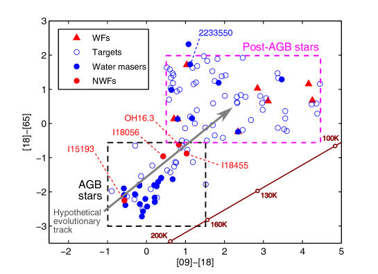
Figure 1: AKARI two-color diagram showing the objects observed in the present survey (open blue circles), the H₂O maser detections (filled blue circles), the water fountains known to date (WFs; red triangles), and the newly identified WF candidates (NWFs; filled red circles). The blackbody curve is indicated by the brown full-line. The estimated boundaries for AGB and post-AGB stars are shown in broken-line boxes. A hypothetical evolutionary track is shown by the grey arrow.

Using known sources, we define the empirical regions of AGB and post-AGB stars on a two-color diagram with AKARI [09]$-$[18] and [18]$-$[65] colors (Figure 1). The known AGB stars (including Mira variables and OH/IR stars) with H₂O maser detections are selected from Engels et al. (1986), Engels & Lewis (1996), Lewis (1997) and Valdettaro et al. (2001). A total of 265 sources are selected. The boundaries are set by the outermost AGB stars distributed on the diagram. For simplicity, a rectangular region is assumed. The same process is used to find out the color region of post-AGB stars. We use 38 post-AGB stars with H₂O maser detections to define the color region. In this sample, 30 of them are selected from Deacon et al. (2007), Suárez et al. (2007), and Suárez et al. (2009). The remaining 8 are the WFs. They are selected because most WFs appear to be post-AGB stars (see Section 1). Note that only 8 WFs have known AKARI fluxes. Therefore, we cannot include all 15 in the AKARI color-color diagram. Post-AGB stars have a much lower H₂O maser detection rate (see, Section 4.1), and there were also not so many corresponding observations, hence the smaller sample we could obtain.

2.2 Categories of Observed Objects

A total of 204 observed objects were selected by different criteria in addition to the empirical regions of the AKARI two-color diagram introduced in Section 2.1. In Table 1, the objects are put into categories (a) to (h), according to their nature. Note that some objects can fall into more than one category.

Category (a). — Contains potential WFs and known WFs. As mentioned in Section 1, the difference between H₂O and OH velocity coverages is a key point to distinguish WFs from other AGB/post-AGB stars. Potential WFs are objects, where previous observations show almost equal velocity coverage of H₂O and OH masers (see the references in Table 1). These marginal cases might turn out to be WFs once extra H₂O maser components are observed at higher velocities. There are 15 objects included.

Categories (b) and (c). — The former category contains AKARI objects (Decl. $\geq-20^{\circ}$) lying inside the post-AGB region in the AKARI two-color diagram (Figure 1), with $0.5\leq[09]$$-$$[18]\leq 4.5$ and $-0.5\leq[18]$$-$$[65]\leq 2$. The latter is similar but for the AGB region in the same diagram, with $-1\leq[09]$$-$$[18]\leq 1.5$ and $-3\leq[18]$$-$$[65]\leq-0.5$ (Figure 1). There are about 350 and 470 objects fulfilling the above criteria for (b) and (c), respectively. However, due to the limited observing time, we have selected only those which are relatively bright in 9 $\mu$m ($>$3 Jy). There are finally 68 and 38 objects included.

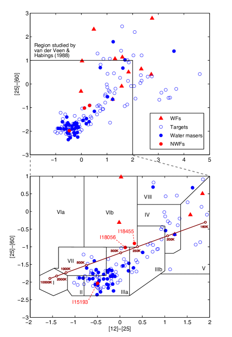
Figure 2: Upper panel: IRAS two-color diagram showing the objects observed in the present survey (open blue circles), the H₂O maser detections (filled blue circles), the water fountains known to date (WFs; red triangles), and 3 of the newly found WF candidates (NWFs; filled red circles). We do not have sufficient information on the IRAS flux of OH 16.3$-$3.0, the forth candidate, thus its position on this diagram is not known. Lower panel: enlarged view of the region studied by van der Veen & Habing (1988). A blackbody curve is indicated by the brown full-line.

Category (d). — Contains IRAS objects (Decl. $\geq-20^{\circ}$) selected from the AGB, post-AGB or redder regions (i.e. IIIa, IIIb, IV, V and VIII) of the IRAS two-color diagram studied by van der Veen & Habing (1988), as shown in Figure 2. The selection method is similar to previous surveys like that of Engels & Lewis (1996), but new samples are added. There are about 360 objects fulfilling the above criteria. We have selected only those which are relatively bright in 12 $\mu$m ($>$5 Jy). There are finally 106 objects included.

Category (e). — Contains known SiO maser sources not observed at 22 GHz before. SiO masers are often detected in oxygen-rich envelopes. These objects are most likely AGB to very early post-AGB stars. There are 98 objects included.

Categories (f) and (g). — Contains H₂O non-detections in two previous major surveys. Category (f) refers to Lewis (1997), and (g) to Johnston et al. (1973). As masers show variability, it often happens that previous non-detections become new detections upon re-observation some years later. Therefore it is worth to revisit some of these objects. It was due to limited observing time that only 6 objects have been observed.

Categories (h). — Contains other sources that do not belong to any of the above categories. These are mainly previously observed objects selected from one of the references for re-observation (see, Table 1). There are 5 objects included.

The columns of Table 1 contain the following information:
Column 1. — Object name.
Columns 2 and 3. — R.A. and Decl. in J2000.0.
Columns 4 and 5. — IRAS [12]$-$[25] and [25]$-$[60] colors, respectively.
Columns 6 and 7. — AKARI [09]$-$[18] and [18]$-$[65] colors, respectively.
Column 8. — The local-standard-of-rest velocity ($V_{\rm LSR}$) of the blueshifted peak of a double-peaked 1612 MHz OH maser profile. For a single-peaked profile, the $V_{\rm LSR}$ is recorded in this column as well, no matter it is really “blueshifted” or not.
Column 9. — $V_{\rm LSR}$ of the redshifted peak of a double-peaked 1612 MHz OH maser profile.
Column 10. — References for the OH maser information given in columns 8 and 9.
Columns 11 and 12. — $V_{\rm LSR}$ of the SiO maser peak in the $(v=1$, $J=1-0)$ and $(v=2$, $J=1-0)$ transitions, respectively.
Column 13. — References for the SiO maser information given in columns 11 and 12.
Column 14. — Category, from (a) to (g), to which the object belongs.

3 Observation and Data Reduction

The observation was performed with the Effelsberg 100 m radio telescope from 2011 November 30 to December 6. An 18–26 GHz HEMT receiver and FFT spectrometer were used in the frontend and the backend, respectively. The rest frequency of the $6_{16}\rightarrow 5_{23}$ transition line of H₂O molecules was adopted as 22.235080 GHz (Lovas, 2004). At this frequency, the full width at half maximum (FWHM) of the beam was about 40″. A 500 MHz bandwidth was used to cover a frequency range from 21.985 to 22.485 GHz ($\sim$6700 km s^-1 at 22.2 GHz). The number of spectral channels was 16,384, yielding a channel spacing of $\sim$0.4 km s^-1. The velocity resolution corresponded to 2 channels, i.e. $\sim$0.8 km s^-1, which was sufficient to spectroscopically resolve each water maser component (normally with a linewidth of $\sim$1–2 km s^-1). By using the 500 MHz bandwidth, we were able to also detect the H66$\alpha$ (with rest frequency 22.364 GHz) and H83$\beta$ (22.196 GHz) recombination lines for certain objects (see, Section 4.2 and Appendix A). The velocity scale has been confirmed to be accurate by comparisons with previous H₂O maser spectra of some known sources.

An ON/OFF cycle of 2 minutes was used in position switching mode. The OFF position was 600″ west from the ON position in azimuthal direction. The observing time for each source was about 6–20 minutes. The weather was fine during most of the observing sessions, and the root-mean-square (rms) noise level was of order $10^{-2}$ to $10^{-3}$ Jy. Pointing was obtained every 1 to 2 hours with a typical accuracy of about 5″. Calibration was obtained from continuum cross scans of sources with flux densities given by Ott et al. (1994).

The data reduction procedures were performed with the Continuum and Line Analysis Single-dish Software (CLASS) package . Individual scans on each object were inspected and those with obvious artifacts were discarded. The remaining scans were then averaged. The baseline of each spectrum was fit by a one-degree polynomial and subtracted, using the channels without emission.

4 Results

4.1 H₂O Maser Detections

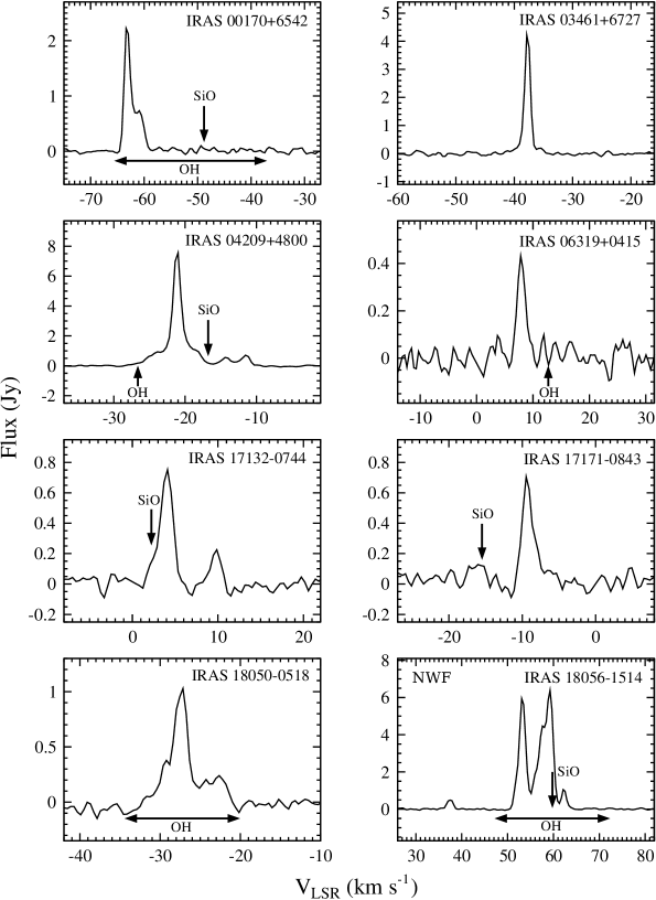
Figure 3: Spectra of new H₂O maser detections. The new “low-velocity” water fountain candidates (IRAS 18056$-$1514, OH 16.3$-$3.0 and IRAS 18455$+$0448) are labeled as “NWF”.

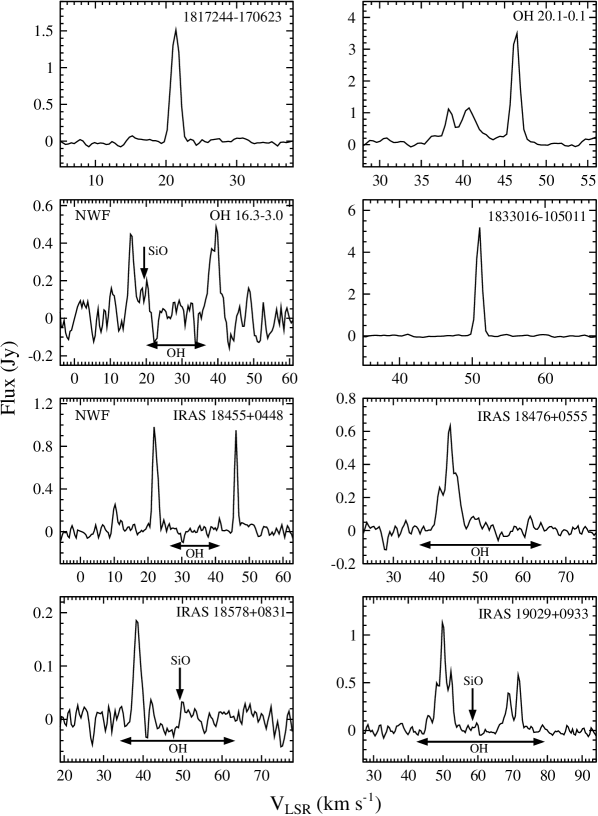
Figure 3: Continued

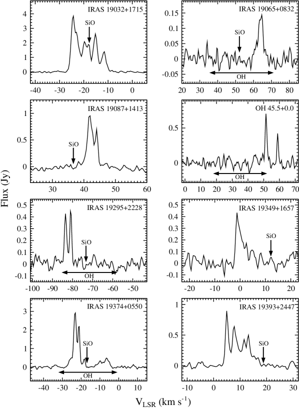
Figure 3: Continued

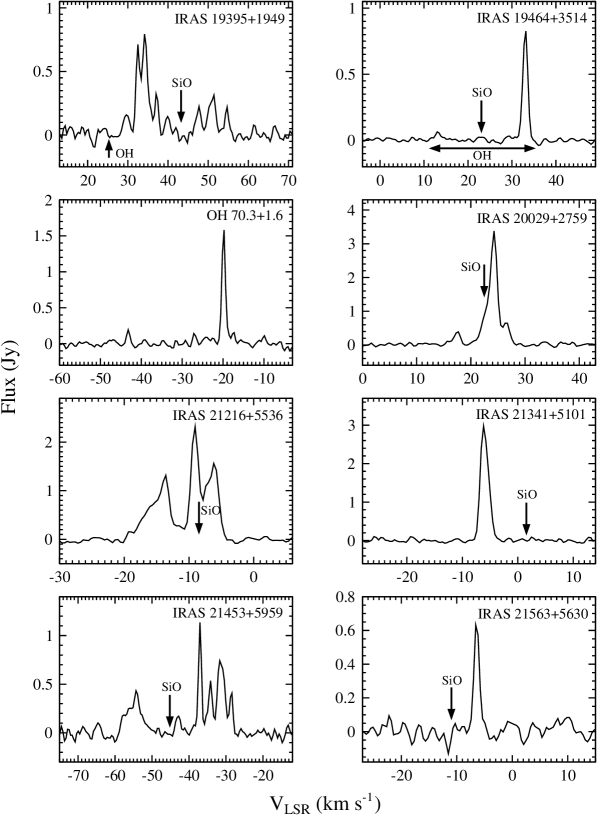
Figure 3: Continued

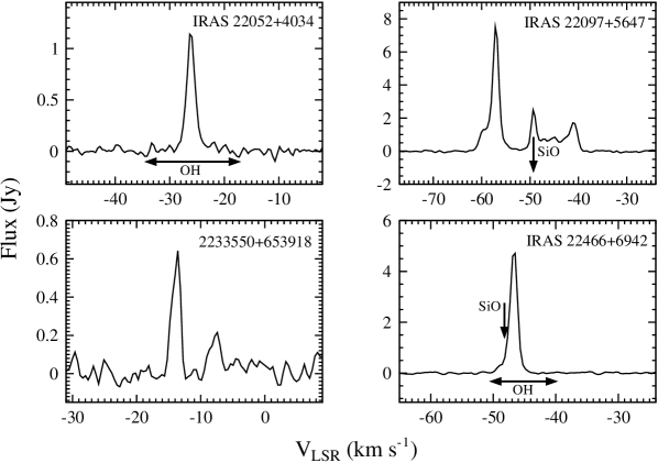
Figure 3: Continued

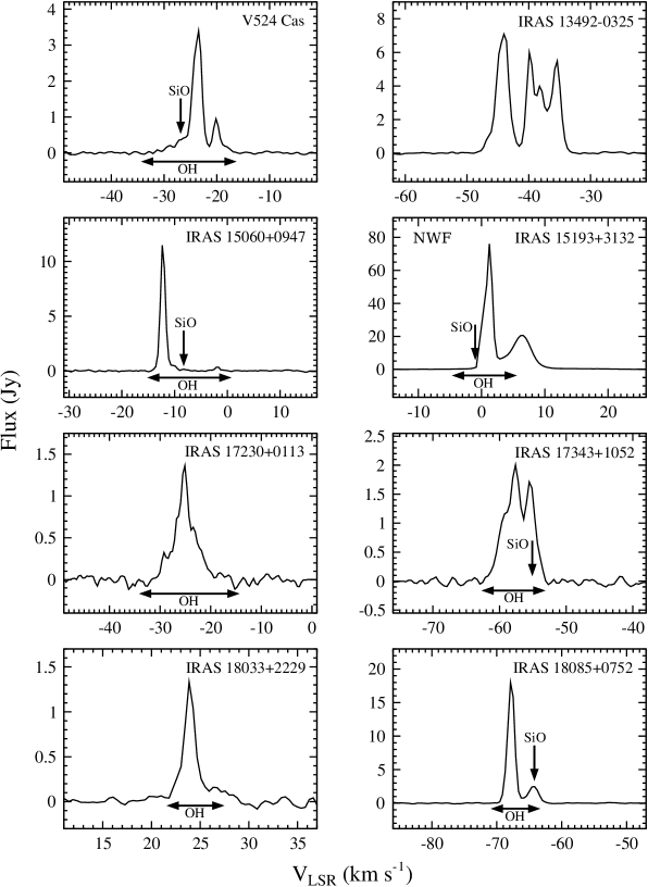
Figure 8: Spectra of revisited known H₂O maser detections. Some of them with new components detected, see Section 4.2 and Appendix A. The new “low-velocity” water fountain candidate (IRAS 15193$+$3132) is labeled as “NWF”.

In this observation, we obtained a total of 63 detections out of 204 objects, and 36 of them are new. Table 2 gives the number of detections in each selection category (see, Section 2.2 and the last column of Table 1). Figure 3 shows the spectra for all the new detections, and Figure 8 shows the spectra for revisited known maser sources. When possible, the velocity range between the two OH maser peaks and the $V_{\rm LSR}$ of the SiO maser feature (if present), are also shown. The parameters of all the H₂O maser detections are given in Table 3. The rms noise level of the non-detections are then given in Table 4.

The new attempt of sample selection using AKARI colors yields a detection rate of 42% for the AGB stars (category (c)), but only about 13% for post-AGB stars (category (b)). This drastic drop of the detection rate towards redder post-AGB stars is expected, and the same tendency was observed in nearly all previous H₂O maser surveys on evolved stars (e.g., Engels & Lewis, 1996; Valdettaro et al., 2001). It is probably due to the decrease in mass-loss rate after the AGB phase, and by the dissociation of the H₂O molecules into OH and H because of the ultra-violet radiation from the central star. The dissociation also happens at a larger distance from the photosphere, but this time it is due to external ultra-violet radiation (Habing, 1996). Categories (d) and (e) consist of objects classified by more traditional ways, i.e., by their IRAS colors or the SiO maser properties. The detection rate is about 35% and 37%, respectively.

We have 6 additional objects from categories (f) and (g). These objects were non-detections in previous observations. We detected H₂O masers from 4 of these. It indicates that the sample selection criteria used by Lewis (1997) and Johnston et al. (1973) were indeed effective. However, Lewis (1997) achieved only a noise level of $\sim$0.3 Jy using the Haystack 37 m radio telescope, and for Johnston et al. (1973), almost 40 years ago, the noise level was up to $\sim$12 Jy for a 5 minute integration using the 26 m reflector of the Maryland Point Observatory.

4.2 Objects with Larger Velocity Coverage of H₂O than OH Masers

Most of the detections in this project have an H₂O velocity coverage smaller than that of OH; this is the behavior of most circumstellar masers (see, Section 1). We found 4 exceptions here. These are IRAS 15193$+$3132 (spectrum in Figure 8), IRAS 18056$-$1514, OH 16.3$-$3.0, and IRAS 18455$+$0448 (Figure 3). These objects show an H₂O velocity coverage which is larger than that for OH, and therefore they are WF candidates. Among the 4 objects, IRAS 15193$+$3132 is a known H₂O maser source, while the other 3 are new sources. There is also another object, OH 45.5$+$0.0, with one of its two narrow H₂O features lying outside the OH interval (Figure 3), but this object is unlikely to be a WF (to be explained later in this sub-section). We have looked at the infrared spectral energy distributions (SEDs) of the 4 candidates. All of them are characterized by a broad thermal emission feature in the mid- to far-infrared range. This is evidence for the presence of a thick envelope, as radiation coming from the central star is absorbed and re-emitted at longer wavelengths. A more extensive study on their SEDs will be presented in another paper (Yung et al. 2013, in preparation). The maser characteristics of the above objects are given below.

IRAS 15193$+$3132 (S CrB). — This is a known H₂O maser source with a double-peaked profile (Valdettaro et al., 2001), which is suggested to be an AGB star with a pulsation period of about 360 days (Shintani et al., 2008). The current observation obtained a velocity coverage from about $1$ to $11$ km s^-1. This is a very bright source, the S/N is over 1000. Its OH maser was first detected by te Lintel Hekkert et al. (1989), which showed a velocity coverage from $-2.5$ to $4.0$ km s^-1. However, in recent OH observations obtained in the year 2012 using the Effelsberg 100 m telescope (data unpublished), we found that the OH coverage should be $-5.0$ to $5.5$ km s^-1 (Figure 8). Nonetheless, it is clear that the H₂O emission exceeds the OH interval on the redshifted side. An SiO maser is located at about $-1$ km s^-1 (Kim et al., 2010). Regarding the distance, the Hipparcos parallex given in the Astrometric Catalog (I/311/hip2) is $1.85\pm 1.19$ mas (van Leeuwen, 2007), implying a distance of about 540 pc, but with a large uncertainty. The total flux calculated from the infrared SED is about $1.0\times 10^{-10}$ W m^-2, corresponding to a luminosity of about 900 $L_{\odot}$. This value is too low for an AGB star (typically $\sim$8000 $L_{\odot}$), and we believe it is not accurate mainly due to the uncertainty in the parallax distance adopted. If the distance is confirmed reliable, then the low luminosity could be a consequence of a late thermal pulse (TP), when the star is becoming a “born-again AGB” star (e.g., Blöcker, 1995). At the early stage of the late TP, the cold envelope is blown away, temporarily exposing the inner part of the star. A larger flux from shorter wavelengths is therefore expected. Nonetheless, at short wavelengths the influence of interstellar extinction is very significant. The total flux observed then decreases, and so does the implied luminosity.

IRAS 18056$-$1514. — There are four H₂O maser peaks associated with this source, three of them are found within the OH velocity interval determined by te Lintel Hekkert (1991a), and one of them is outside. The S/N of the dimmest peak is about 21 (Figure 3). If we take the central velocity of the OH masers as the systemic velocity of the star, then the most blueshifted H₂O emission (at $\sim$36 km s^-1) implies a projected outflow velocity of about 23 km s^-1. The expected redshifted peak is missing, but since masers show variation, the peak is not detected probably because it is at its minimum. An SiO maser ($v=2$, $J=1-0$ transition only) is detected near the adopted systemic velocity, at about 60 km s^-1 (Deguchi et al., 2000). The kinematical distance estimated using the systemic velocity and the galactic rotation curve (Kothes & Dougherty, 2007) is about 4.0 kpc. Note that the kinematical distance also includes a large uncertainty. The total infrared flux and the luminosity are about $4.6\times 10^{-12}$ W m^-2 and 2300 $L_{\odot}$, respectively.

OH 16.3$-$3.0. — This object shows a double-peaked profile for both H₂O and OH masers. The S/N of the H₂O peaks is about 5 (Figure 3). For OH, “Wing-like” features were found in the outer side of both peaks (Sevenster et al., 2001). The velocity coverage between the two OH peaks is about 17 km s^-1, while for H₂O it is about 29 km s^-1. The OH peaks tell the expansion velocity, so the “wings” are probably a sign of a fast outflow, and the most plausible case is a bipolar outflow. An SiO maser was found at about $-19$ km s^-1, with the 45 m telescope of the Nobeyama Radio Observatory (NRO) on 2012 March 18 (Nakashima 2012, private communication). It has to be noted that the SiO maser is not located at the supposed systemic velocity (i.e. the velocity halfway between the two OH peaks), but it has a similar velocity as one of the OH peaks. The kinematical distance, total flux and luminosity of the object are estimated to be 2.6 kpc, $9.0\times 10^{-12}$ W m^-2 and 2000 $L_{\odot}$, respectively.

IRAS 18455$+$0448. — The OH maser profile of this object was first analyzed by Lewis et al. (2001). They found that the double-peaked feature was fading away over a period of 10 years, and this object has been argued to be a very young post-AGB star. The OH velocity coverage is about 14 km s^-1. No H₂O masers were detected in the survey conducted by Engels & Lewis (1996). Our new H₂O spectrum (Figure 3) consists of two dominant peaks located on each side of the OH interval, and one additional blueshifted peak farther away from the systemic velocity. The S/N of the dimmest peak is about 7, and the total H₂O velocity coverage is about 39 km s^-1. No SiO masers were detected (Nakashima 2012, private communication). The near and far kinematical distances are 1.9 and 12 kpc, respectively. Lewis et al. (2001) suggested that in this case the far distance was more likely to be correct. It is because if one assumes the near distance, the luminosity would be very low ($\sim$400 $L_{\odot}$), which contradicts to the post-AGB star status that is supported by other evidence (e.g. by the behavior of the 1612 and 1667 MHz OH profiles). Adopting 12 kpc, the total flux and luminosity of the object are estimated to be $3.6\times 10^{-12}$ W m^-2 and 16,000 $L_{\odot}$, respectively.

OH 45.5$+$0.0. — The H₂O spectrum (Figure 3) shows two narrow peaks at about 51 and 58 km s^-1, and one of them is outside the interval covered by the OH masers (18–53 km s^-1). The H66$\alpha$ and H83$\beta$ recombination lines are also detected within the 500 MHz bandwidth. When the spectra are set to the corresponding rest frequencies, both lines with broad profiles are centered at about 50 km s^-1 (i.e. agree with the strongest H₂O feature).

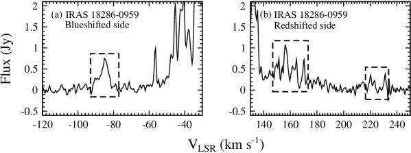
Figure 12: Close-up view of the H₂O maser spectrum of the WF IRAS 18286$-$0959 on the (a) blueshifted, and (b) redshifted sides. The new velocity components are indicated by the broken-line boxes.

In addition, new high velocity H₂O maser components are found in the known WF IRAS 18286$-$0959 (Figure 8, and a close up view in Figure 12), when comparing with our previous spectra obtained in years 2008 to 2010 with the Very Long Baseline Array (VLBA) and the NRO 45 m telescope. IRAS 18286$-$0959 has a precessing jet, which exhibits a unique “double-helix” pattern revealed by interferometric observations (Yung et al., 2011). The H₂O spectrum has an irregular profile with a lot of bright peaks. The new components are weak, but they are still well above the 5-$\sigma$ limit, with a noise level about $5.31\times 10^{-2}$ Jy. The original velocity coverage is from about $-60$ km s^-1 to $160$ km s^-1. Now we see emission between $-92$ km s^-1 and $171$ km s^-1. The coverage has increased from $220$ km s^-1 to $263$ km s^-1, surpassing IRAS 16342$-$3814 ($\sim$250 km s^-1, Claussen et al., 2009). The velocity coverage is now the forth largest among the 15 WFs. Only the H₂O emissions from IRAS 18113$-$2503 ($\sim$500 km s^-1, Gómez et al., 2011), OH 009.1$-$0.4 ($\sim$400 km s^-1, Walsh et al., 2009), and IRAS 18460$-$0151 ($\sim$300 km s^-1, Deguchi et al., 2007) are distributed over a wider range. Therefore, the actual velocity of the jet could be faster than the currently adopted value (i.e., about 140 km s^-1, Yung et al., 2011), but probably due to the variability of the maser flux, these components were not detected before. Note that the observations committed in 2008 to 2010 have achieved a similar sensitivity as the current one (rms $\sim 10^{-2}$ Jy), so that the possibility of the new peaks being overlooked from previous work is excluded. On the other hand, the jet could indeed accelerate. However, that would imply an increase of $>$40 km s^-1 of the jet velocity in 1–2 years. It would be remarkable if true, because there were no such extreme accelerations ever found in evolved stars. Jet acceleration is possible as it is already found in the proto-PN CRL 618 (Sánchez Contreras et al., 2004) and another WF OH 12.9$-$0.9 (Boboltz & Marvel, 2005), but there the acceleration is $<$10 km s^-1 per year. Since the jet of IRAS 18286$-$0959 is precessing, it is also possible that the velocity coverage is affected by the jet direction and shows time variation. However, according to our kinematical model (Yung et al., 2011), an increase of $\sim$40 km s^-1 is difficult to explain by pure precession within 2 years.

4.3 The Unclassified Object 2233550$+$653918

2233550$+$653918 is located in the post-AGB region of the AKARI two-color diagram (Figure 1). It has a near-infrared counterpart in the 2MASS catalog, but not in IRAS and MSX catalogs. Its WISE image appears to be a stellar point source. No SIMBAD papers are found regarding this object, so it is completely new to us. It has a double-peaked H₂O maser profile spreading about 10 km s^-1 (Figure 3). The S/N are about 16 and 6 for the blueshifted and redshifted peak, respectively. The true nature of this object is unknown but it might be an evolved star (more in Section 5.1). After the observation, we have found a few more objects with similar infrared properties (i.e. with post-AGB colors in the AKARI diagram; no IRAS and MSX counterparts, and no related studies are found). It shows that the high sensitivity of AKARI does enable us to find completely new maser sources, which could be post-AGB star candidates.

5 Discussion

5.1 Confirmation of the Evolved Star Status

Some star forming regions (SFRs) exhibit H₂O maser profiles or even infrared colors that resemble those of late-type objects such as post-AGB stars, so that misidentifications are possible. Furthermore, when the objects are close to the Galactic Plane, contamination by other sources may also occur. Therefore, first of all, we have to consider the evolved star status of the newly found WF candidates (especially IRAS 18056$-$1514, OH 16.3$-$3.0, and IRAS 18455$+$0448). Their physical properties as WF are then discussed in later subsections.

We found that there are no other known red sources in IRAS, MSX, AKARI, or WISE catalogs except the target sources within the main beam of the telescope, so the possibility of contamination is firstly excluded. Then, we confirmed that there were no 21 cm continuum sources (i.e. Hii regions) toward the corresponding directions of the 4 WF candidates (Condon et al., 1998). That implies these maser sources are not high-mass SFRs. There are also no reports on any OH masing low-mass SFR (Garay & Lizano, 1999; Sahai et al., 2007), so the candidates are unlikely to be low-mass SFRs as well. The estimated luminosities given in Section 4.2 might not be accurate due to the uncertainties in the adopted distances. However, even in the extreme case of having 50% of distance uncertainty, the luminosities of all those objects are still brighter than the typical value ($<$100 $L_{\odot}$) for a young stellar object. In addition, they appear as point sources in MSX and WISE mid-infrared images, which are very different from SFRs that normally show large irregular extended features.

Among the other new H₂O sources, 1817244$-$170623, OH 20.1$-$0.1 OH 45.5$+$0.0, and OH 70.3$+$1.6 are found to be lying in Hii regions. OH 45.5$+$0.0 (Section 4.2) and OH 70.3$+$1.6 (Appendix A) are the only objects toward which the H66$\alpha$ and H83$\beta$ recombination lines have been detected. These lines are detected in highly ionized regions. Note that some recombination lines are also found in PNe (e.g., Roelfsema et al., 1991). Nonetheless, OH 45.5$+$0.0 and OH 70.3$+$1.6 are unlikely to be PNe because of their highly irregular shape as shown in mid-infrared images. In addition, PNe are known to have a very low detection rate of H₂O masers due to the short lifetime ($\sim$100 years) of H₂O molecules in the PN environment (e.g., de Gregorio-Monsalvo et al., 2004). Thus, the above two objects are more likely to be SFRs. There are no detailed studies on 1833016$-$105011, but its mid-infrared images reveal small nebulosity around the central object.

The rest of the new sources, including 2233550$+$653918 (Section 4.3), are most probably evolved objects because of their point-source-like appearance in mid-infrared images, as well as the non-detection of 21 cm continuum emission. The SiO maser detections toward some of the objects provide additional evidence for their evolved star status (e.g., Nakashima & Deguchi, 2003a). The 3 exceptional cases where SiO masers are detected toward SFRs are Orion-KL (Kim et al., 2008), Sgr B2 (Shiki et al., 1997) and W51-IRS2 (Morita et al., 1992). Category (d) of our sample consists of some known SiO maser sources (see Table 1).

5.2 Properties of the New Water Fountain Candidates

In Section 1, we mentioned that the smaller H₂O velocity coverage of the low-velocity WFs could be just a projection effect on high velocity jets, or the jets are intrinsically slower. For the 4 candidates reported in this paper, we suggest below that they are more likely to possess slow jets, and they are younger than other known WFs in terms of evolutionary status. Not knowing the true three-dimensional jet velocity yet, we will justify our idea by considering infrared colors and maser kinematics. Observations using very long baseline interferometry (VLBI) will be needed for further analysis.

5.2.1 AKARI and IRAS Colors

Based on the distribution of the AGB and post-AGB stars in Figure 1, we can assume a rough stellar evolutionary track in the diagram. This is because when an AGB star evolves further, its mass-loss will create a very thick dust envelope which obscures the central star. The object will become very dim, or even unobservable, in optical and near-infrared ranges. On the contrary, it becomes relatively bright in the mid-infrared due to the cold outer envelope. Hence, late AGB and early post-AGB stars normally show very red colors (e.g., Deguchi et al., 2007). As a result, the evolving AGB stars will move toward the “upper-right” direction in a two-color diagram, when their colors become redder. This evolutionary direction agrees with the model prediction by Suh & Kwon (2011). The same tendency is also noted in the IRAS two-color diagram presented by van der Veen & Habing (1988).

From Figure 1, the new WF candidates are expected to be less evolved than most of the other WFs, but at the same time, at least 3 of them have been departed from the main cluster of AGB stars used in our sample. IRAS 18056$-$1514, OH 16.3$-$0.3 and IRAS 18455$+$0448 were originally selected by their AKARI colors, and incidentally, they are located at the upper-right corner of the AGB star region on the AKARI two-color diagram (see Figure 1), and they are not as red as the confirmed WFs in both color indices. The colors of these 3 candidates indicate that they could be transitional objects at the late AGB/early post-AGB stage. The remaining candidate, IRAS 15193$+$3132, lies in the AGB region of the AKARI two-color diagram, which is consistent with its suggested AGB status.

The IRAS two-color diagram suggests a similar story (Figure 2). IRAS 15193$+$3132 is found in region IIIa, while IRAS 18056$-$1514 and IRAS 18455$+$0448 are found at the boundaries between region IIIa, IIIb and VIb. OH 16.3$-$0.3 is missing because the 60 $\mu$m flux is not known. According to van der Veen & Habing (1988), variable stars with thick O-rich envelopes are found in region IIIa and IIIb. These are very likely late AGB stars, where thick envelopes are formed due to the mass-loss. Region VIb contains variable stars with hot dust close to the photosphere, and cold dust at larger distances. These could be early post-AGB stars, where the steady spherical mass-loss has been interrupted, and the dust far away from the central star has cooled down.

5.2.2 Maser Kinematics

If we believe that the new candidates are less evolved than other WFs, the next question is about their jet velocities. The fact that the H₂O maser velocity coverage is larger than OH implies a physical differentiation of the faster H₂O maser flow (probably bipolar) from the circumstellar OH flow. From the spectra, we are not able to determine the three-dimensional velocity. Nonetheless, we can argue that the chance of the new candidates to be associated with high velocity jets is rather low, by considering the orientation of the jet axes. Most WFs are found to have a three-dimensional jet velocity in the range of $100\leq V\leq 250$ km s^-1 (e.g., Imai et al., 2007; Walsh et al., 2009; Gómez et al., 2011). The projected velocity is given by $V\cos(i)$, where $i$ (from $0^{\circ}$ to $90^{\circ}$) is the inclination angle between the jet axis and the line-of-sight. If a low-velocity WF has an H₂O maser velocity coverage about 30 km s^-1, then the projected velocity of the maser peaks will be 15 km s^-1 (half of the total velocity coverage) off the systemic velocity. For jet velocities $V=100$, 150, or 250 km s^-1, we obtain $i\approx 81^{\circ}$, $84^{\circ}$, or $87^{\circ}$, respectively. Among the candidates that we have found, 3 of them have a velocity coverage of even less than 30 km s^-1 (except IRAS 18455$+$0448). Therefore the inclination angle should be at least $81^{\circ}$ for a 100 km s^-1 jet, or even larger for higher velocity jets.

We can estimate the probability of seeing such a jet in the following way. Assume that there is no bias in the jet axis direction in the three-dimensional space, so that jets with different orientations are distributed uniformly across the sky. Then the probability $P(i_{1},i_{2})$ of observing a jet with an inclination angle between $i_{1}$ and $i_{2}$ (for $i_{1}<i_{2}$) is given by

$$P(i_{1},i_{2})=\frac{1}{2\pi}\int_{0}^{2\pi}\int_{i_{1}}^{i_{2}}\sin(i)\,{\rm d}i\,{\rm d}\phi~{},$$ (1)

where $\phi$ is the azimuthal angle defined on the sky plane. For the extreme projection examples described above (i.e. $i_{1}=81^{\circ},84^{\circ}$ or $87^{\circ}$; $i_{2}=90^{\circ}$), the probabilities calculated by the formula are about 17%, 10%, or 5%. On the other hand, the total number of WFs and WF candidates is $15+4=19$. Thus, about $5/19=26\%$ of them are low-velocity WFs (including OH 12.8$-$0.9), which is higher than the calculated probabilities. Hence, the small H₂O velocity coverages are probably not caused by pure geometrical effects, and the objects are likely to have intrinsic slow jets.

According to the known cases of jet acceleration in OH 12.8$-$0.9 and CRL 618 (Section 4.2), we could assume that the very “first” bipolar outflow from a late AGB star might actually occur with a lower velocity, then it gradually accelerates. This is consistent with our interpretation that the new WF candidates are younger and possess slower jets than other known WFs. The acceleration mechanism is still not clear, but there exist mechanisms like that proposed by the magnetocentrifugal launching  (MCL) model (see, Dennis et al., 2008, and references therein). The MCL model assumes the system has a rotating central gravitating object (the central star), which may or may not include an accretion disk. For the case that the disk is present (which is quite common in post-AGB stars), plasma is threaded by a magnetic field whose poloidal component is rotating in the same direction as the disk. The ionized gas of the disk is then subject to centrifugal force and accelerates. The gas is thrown out along the field lines. As the system expands, the toroidal component of the field dominates and the hoop stress (or circumferential stress) collimates the outflow. Note that a magnetic field ($B\approx 200$ mG at one position along the jet) has already been detected toward W 43A, the first candidate of the WF class (Vlemmings et al., 2006). Therefore, it is possible that magnetic fields play a major role in collimating as well as accelerating the jets. If such acceleration is occurring, then the existence of the low-velocity WF candidates will imply that the dynamical age of WFs should be much larger than what has been expected (less than 100 years, Imai, 2007), because the current adopted value was estimated only with the high jet velocities.

Finally, regarding the SiO masers of the new WF candidates, we note that IRAS 18056$-$1514 has an SiO emission line at the systemic velocity. The fact that only the $v=2$ line has been detected is consistent with the late AGB/early post-AGB phase prediction, as Nakashima & Deguchi (2003a) found that the SiO $v=2$ line will become dominant as the objects get redder in their IRAS colors (i.e. more evolved objects). IRAS 15193$+$3132 also exhibits an SiO maser feature at about the systemic velocity, but only the $v=1$ line has been measured (Table 1). The behavior of its SiO and OH masers also agree with its AGB status. It implies that the onset of an asymmetric outflow (as indicated by the H₂O and OH maser profiles) could actually happen at a stage much earlier than the post-AGB phase. The other 2 candidates show either SiO non-detections, or the emission peak is seen off the systemic velocity. We suggest this is due to the preliminary morphological change, when the envelopes start to develop bipolarity. The SiO masers at this stage are probably originated from an elongated region, and a double-peaked profile is expected even though we only have a single peak for OH 16.3$-$3.0. A similar example is the bipolar SiO outflow of the late AGB star W 43A, which has been mapped with the Very Large Array (Imai et al., 2005). This stage, however, is expected to be short. As the star evolves further and the envelope is detached from the star the SiO maser will disappear. This could be the case of IRAS 18455$+$0448 and the rest of the WFs. Therefore, considering all the properties discussed, the new WF candidates could be characteristic representatives of the short transition stage at the late AGB/early post-AGB phase, when the morphology of the envelopes starts to develop asymmetry.

6 Conclusions

We have conducted a 22 GHz water maser survey on 204 objects, mainly AGB and post-AGB stars, using various source selection criteria such as the AKARI two-color diagram. There are 63 detections and 36 of them are new, including an unclassified object that was first identified by the AKARI observations, 2233550$+$653918. New high velocity components are also found in the known “water fountain” IRAS 18286$-$0959. We have found 4 new candidates for this water fountain class, but having much smaller H₂O maser velocity coverage than other known examples. In principle, the smaller velocity coverage could just be a projection effect, or the objects are really associated with slower jets. From our statistics, we suggest that they are more likely to have intrinsic slow jets. They could be transitional objects undergoing a morphological change, during the late AGB/early post-AGB stage. Studying the kinematical process occurring at this stage is helpful for us to understand the shaping of planetary nebulae. Nonetheless, the true status of the candidates can only be confirmed upon interferometric observations, or by high resolution infrared imaging, to see whether there are bipolar structures or not. The three-dimensional velocity of the outflow could also be determined by measuring the proper motions of the maser features, with multi-epoch VLBI observations (e.g., Imai et al., 2002; Yung et al., 2011).

Appendix A Other Notable H₂O Maser Detections

There are some notable sources in addition to the new water fountain (WF) candidates found in this project, which will be briefly described below:

IRAS 06319$+$0415 (RAFGL 961). — This is a well known object suggested to be a massive protostar, made famous by the detection of the water ice vibrational band (e.g., Smith & Wright, 2011). It is however, the first time that an H₂O maser is found.

OH 70.3$+$1.6. — It has two H₂O maser peaks. We suggest it is a high mass star forming region (SFR), as the H66$\alpha$ (22.364 GHz) and H83$\beta$ (22.196 GHz) recombination lines are detected within our 500 MHz bandwidth. Both lines are centered at about $-30$ km s^-1 (i.e. roughly halfway between the velocities of the two H₂O peaks). These lines only occur in highly ionized Hii region. The object also shows characteristic extended features in mid-infrared images, which agrees with the SFR assumption.

IRAS 19271$+$1354. — This object has two clusters of H₂O peaks. The detection of the blueshifted cluster is reported in Engels & Lewis (1996), and the present observation is the first time that the more redshifted cluster is detected. A single-peaked feature was found in both the OH (Chengalur et al., 1993) and SiO (Nakashima & Deguchi, 2003b) spectra, and the velocities of both emission peaks are lying outside the H₂O velocity range. The SiO maser resembles that of the new WF candidate OH 16.3$-$3.0 (i.e. significantly drifted away from the assumed systemic velocity). The object might have started to develop asymmetry in the very inner part of the envelope. Nonetheless, lacking fully convincing evidence, we conservatively do not suggest it is a WF candidate. To prove its true status, we have to at least detect both OH peaks and get the accurate envelope expansion velocity.

IRAS 19295$+$2228. — This object is identified as an OH/IR star, and it is visually close ($\sim$130″) to another object with similar nature, IRAS 19296$+$2227. Their OH masers were observed in the same beam and recorded with the designation OH 57.5$+$1.8. However, Engels (1996) found that the 2 clusters of OH masers, with very different line-of-sight velocities, actually belong to 2 different sources. H₂O maser emission was found in IRAS 19296$+$2227, but not in IRAS 19295$+$2228 (Engels & Lewis, 1996). Therefore, here we present the first detection in H₂O toward IRAS 19295$+$2228. In addition, Nakashima & Deguchi (2003a) searched for 43 GHz SiO masers toward both objects, but it was only found in IRAS 19295$+$2228.

IRAS 19312$+$1950. — A new H₂O peak at 26 km s^-1 is added to the known double-peaked profile of this source. Currently there are several speculations about the true nature of this peculiar object: it could be a post-AGB star embedded in a small dark cloud by chance, a red nova formed by a merger of two main sequence stars, or a coincidence of a background/foreground small dark cloud appearing in the direction of the IRAS source with the same $V_{\rm LSR}$. Upon interferometric observations, it is shown that the two original H₂O peaks correspond to a possible bipolar outflow (see, Nakashima et al., 2011, for a detailed study of this object). It is unclear how the new peak is produced in the system.

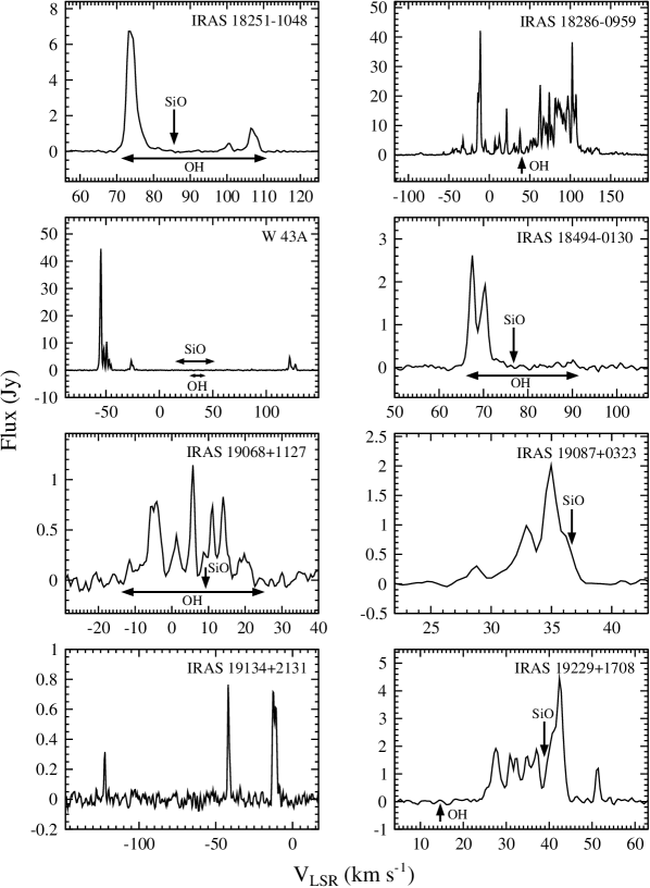
Figure 4: Continued

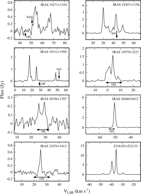
Figure 4: Continued

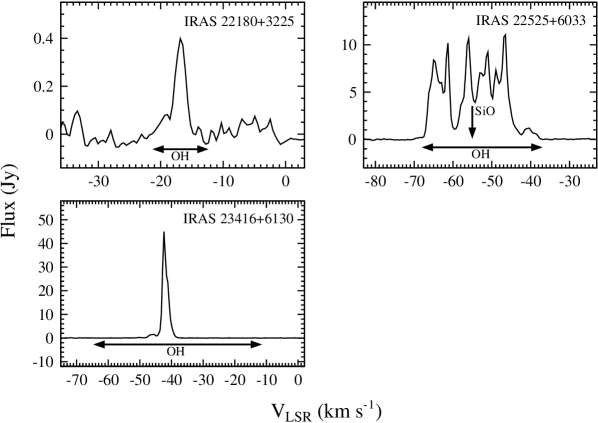
Figure 4: Continued

Table 1: Parameters of the observing targets. Non-detections are denoted by ‘N’, and a blank entry means there were no corresponding observations carried out before.

Object	R.A.	Decl.	IC12	IC23	AC12	AC23	OH $V_{\rm b,p}$	OH $V_{\rm r,p}$	Ref. 1	SiO $V_{\rm LSR}$ 1	SiO $V_{\rm LSR}$ 2	Ref. 2	Cat.
							( km s-1)	( km s-1)		( km s-1)	( km s-1)
IRAS 23575$+$2536	00 00 06.56	$+$25 53 11.2	$-0.94$	$-2.08$	$-0.83$	$\cdots$	N	N	$1$	$-29.2$	$-29.1$	$2$	e
IRAS 00170$+$6542	00 19 51.28	$+$65 59 30.4	$0.19$	$-1.68$	$0.26$	$-1.84$	$-65.0$	$-37.6$	$3$	$-48.9$	$-51.0$	$4$	d,e
V 524CAS	00 46 00.12	$+$69 10 53.4	$-0.36$	$-1.78$	$-0.09$	$-2.57$	$-34.8$	$-16.5$	$5$	$-27.0$	$\cdots$	$6$	c,e
IRAS 01572$+$5844	02 00 44.10	$+$58 59 03.0	$-0.50$	$-1.86$	$\cdots$	$\cdots$	$-19.8$	$-2.9$	$7$	$\cdots$	$\cdots$	$\cdots$	d
IRAS 02547$+$1106	02 57 27.48	$+$11 18 05.7	$-0.09$	$-1.71$	$-0.31$	$-2.22$	$6.4$	$25.4$	$1$	$\cdots$	$\cdots$	$\cdots$	c,d
IRAS 03022$+$5409	03 05 52.91	$+$54 20 53.9	$-0.43$	$-2.18$	$-0.30$	$\cdots$	$\cdots$	$\cdots$	$\cdots$	N	N	$8$	d,e
IRAS 03206$+$6521	03 25 08.80	$+$65 32 07.0	$0.36$	$-1.38$	$0.71$	$-1.26$	$-47.0$	$-28.0$	$3$	$-40$	$-37.8$	$6,9$	b,d,e
IRAS 03461$+$6727	03 50 57.00	$+$67 36 50.0	$-0.74$	$-1.60$	$-0.64$	$\cdots$	$\cdots$	$\cdots$	$\cdots$	$\cdots$	$\cdots$	$\cdots$	f
IRAS 04209$+$4800	04 24 40.40	$+$48 07 24.2	$-0.28$	$-1.91$	$-0.57$	$-2.09$	$-26.4$	$\cdots$	$7$	$-16.8$	$-16.7$	$9$	c,d,e
IRAS 05131$+$4530	05 16 47.10	$+$45 34 04.0	$0.61$	$-1.29$	$0.61$	$-1.43$	$-42.8$	$-22.9$	$3$	N	$-30.5$	$8$	c,d,e
IRAS 05284$+$1945	05 31 24.70	$+$19 47 19.0	$0.83$	$-1.07$	$0.51$	$\cdots$	$2.6$	$27.0$	$10$	$14.2$	$14.6$	$9$	d,e
IRAS 05506$+$2414	05 53 43.59	$+$24 14 44.4	$\cdots$	$\cdots$	$1.27$	$1.20$	$0.5$	$10.1$	$1$	$\cdots$	$\cdots$	$\cdots$	b
IRAS 05552$+$1720	05 58 07.51	$+$17 20 58.5	$\cdots$	$\cdots$	$-0.07$	$\cdots$	$31.8$	$57.7$	$1$	$42.2$	$45.1$	$9$	b,e
IRAS 06121$+$1221	06 14 59.40	$+$12 20 16.0	$\cdots$	$\cdots$	$\cdots$	$\cdots$	$82.3$	$\cdots$	$1$	$\cdots$	$\cdots$	$\cdots$	h
IRAS 06238$+$0904	06 26 37.26	$+$09 02 14.9	$-0.72$	$-1.48$	$-0.89$	$-1.98$	$26.0$	$\cdots$	$1$	$\cdots$	$\cdots$	$\cdots$	c,d
IRAS 06319$+$0415	06 34 37.63	$+$04 12 42.8	$1.70$	$1.02$	$1.68$	$\cdots$	$12.7$	$\cdots$	$1$	N	N	$11$	d
0759401$+$152312	07 59 40.13	$+$15 23 12.4	$\cdots$	$1.61$	$1.30$	$1.68$	$\cdots$	$\cdots$	$\cdots$	$\cdots$	$\cdots$	$\cdots$	b
IRAS 13492$-$0325	13 51 51.66	$-$03 40 34.0	$-0.82$	$-1.89$	$-0.74$	$\cdots$	N	N	$12$	N	$\cdots$	$13$	d
IRAS 15060$+$0947	15 08 25.70	$+$09 36 18.0	$-0.29$	$-2.06$	$-0.17$	$-2.36$	$-16.3$	$1.8$	$1$	$-8.2$	$-8.3$	$14$	a,b,d,e
IRAS 15193$+$3132	15 21 23.30	$+$31 22 02.0	$-0.51$	$-2.04$	$-0.57$	$-2.28$	$-5.0$	$5.5$	$\cdots$	$-1.1$	$-1.2$	$15$	a,d,e
IRAS 16030$-$0634	16 05 46.33	$-$06 42 27.9	$-0.64$	$-1.73$	$-0.46$	$\cdots$	$\cdots$	$\cdots$	$\cdots$	$-6.0$	$-6.4$	$16$	e
1611445$+$120416	16 11 44.55	$+$12 04 16.6	$\cdots$	$\cdots$	$3.56$	$0.36$	$\cdots$	$\cdots$	$\cdots$	$\cdots$	$\cdots$	$\cdots$	b
IRAS 16131$-$0216	16 15 47.66	$-$02 23 31.9	$-0.72$	$-1.90$	$-0.64$	$\cdots$	$\cdots$	$\cdots$	$\cdots$	$60.3$	$60.2$	$14$	d,e
1644295$+$234759	16 44 29.51	$+$23 47 59.8	$2.75$	$0.32$	$2.42$	$0.83$	N	N	$17$	$\cdots$	$\cdots$	$\cdots$	b
IRAS 17055$-$0216	17 08 10.20	$-$02 20 21.0	$-0.19$	$-1.89$	$-0.22$	$\cdots$	$\cdots$	$\cdots$	$\cdots$	$-40.6$	$-40.1$	$16$	d,e
IRAS 17132$-$0744	17 15 56.40	$-$07 47 33.0	$-0.50$	$-2.03$	$\cdots$	$\cdots$	$\cdots$	$\cdots$	$\cdots$	$2.1$	$3.7$	$16$	d,e
IRAS 17171$-$0843	17 19 53.45	$-$08 46 59.7	$-0.26$	$-2.08$	$-0.11$	$\cdots$	N	N	$18$	$-15.5$	$-15.6$	$16$	d,e
IRAS 17193$-$0601	17 22 02.30	$-$06 04 13.0	$-0.46$	$-1.88$	$-0.46$	$\cdots$	$\cdots$	$\cdots$	$\cdots$	$-36.5$	$-35.8$	$16$	d,e
IRAS 17230$+$0113	17 25 36.51	$+$01 11 06.0	$-0.17$	$-1.84$	$-0.13$	$\cdots$	$-34.6$	$-14.4$	$1$	$\cdots$	$\cdots$	$\cdots$	d
IRAS 17308$+$0822	17 33 13.90	$+$08 20 41.0	$0.05$	$-1.55$	$0.52$	$\cdots$	$1.9$	$14.7$	$1$	$8.1$	$8.0$	$19$	d,e
IRAS 17343$+$1052	17 36 44.50	$+$10 51 05.0	$-0.90$	$-1.88$	$-0.72$	$\cdots$	$-62.6$	$-53.1$	$1$	$-55.3$	$-55.4$	$19$	a,e
1744554$+$500239	17 44 55.44	$+$50 02 39.5	$3.70$	$-0.21$	$4.36$	$0.58$	N	N	$20$	$\cdots$	$\cdots$	$\cdots$	b
1749069$+$080610	17 49 06.91	$+$08 06 10.2	$1.11$	$1.07$	$1.18$	$1.63$	$\cdots$	$\cdots$	$\cdots$	$\cdots$	$\cdots$	$\cdots$	b
IRAS 17484$-$1511	17 51 20.38	$-$15 12 26.6	$0.74$	$-0.95$	$1.19$	$-1.13$	$77.0$	$110.1$	$10$	N	N	$21$	c,d
IRAS 17531$-$0940	17 55 53.10	$-$09 41 24.0	$0.73$	$-1.14$	$0.74$	$\cdots$	$18.6$	$43.6$	$3$	$\cdots$	$\cdots$	$\cdots$	d
1758333$+$663759	17 58 33.39	$+$66 37 59.9	$\cdots$	$\cdots$	$2.54$	$0.78$	N	N	$22$	$\cdots$	$\cdots$	$\cdots$	b
1800071$+$663654	18 00 07.14	$+$66 36 54.3	$\cdots$	$\cdots$	$1.93$	$1.38$	$\cdots$	$\cdots$	$\cdots$	$\cdots$	$\cdots$	$\cdots$	b
IRAS 18033$+$2229	18 05 26.60	$+$22 30 04.0	$\cdots$	$\cdots$	$-0.63$	$\cdots$	$21.9$	$27.3$	$1$	$\cdots$	$\cdots$	$\cdots$	a
IRAS 18050$-$0518	18 07 41.03	$-$05 18 19.6	$-0.16$	$-2.06$	$0.21$	$-2.30$	$-34.2$	$-20.3$	$18$	$\cdots$	$\cdots$	$\cdots$	c,d
IRAS 18056$-$1514	18 08 28.40	$-$15 13 30.0	$0.12$	$-1.02$	$0.43$	$-0.96$	$46.7$	$72.1$	$18$	N	$59.7$	$23$	c,e
IRAS 18085$+$0752	18 10 58.50	$+$07 53 09.0	$-0.55$	$-2.07$	$-0.43$	$\cdots$	$-71.2$	$-63.5$	$1$	N	$-64.1$	$19$	a,d,e
IRAS 18095$+$2704	18 11 30.67	$+$27 05 15.5	$1.12$	$-1.64$	$1.52$	$-1.78$	$-12.7$	$0.9$	$1$	N	N	$21$	c,d
1812063$+$065113	18 12 06.34	$+$06 51 13.1	$2.11$	$-0.62$	$2.47$	$-0.19$	N	N	$22$	$\cdots$	$\cdots$	$\cdots$	b
IRAS 18099$-$1449	18 12 47.37	$-$14 48 50.0	$-0.07$	$\cdots$	$-0.68$	$\cdots$	$\cdots$	$\cdots$	$\cdots$	$1.7$	$-0.5$	$14$	e
IRAS 18100$-$1250	18 12 50.49	$-$12 49 44.8	$-0.19$	$\cdots$	$-0.39$	$\cdots$	$\cdots$	$\cdots$	$\cdots$	$80.2$	$79.5$	$14$	e
IRAS 18117$-$1625	18 14 38.70	$-$16 24 39.0	$0.23$	$\cdots$	$0.04$	$\cdots$	$\cdots$	$\cdots$	$\cdots$	$85.1$	$84.8$	$23$	e
IRAS 18118$-$1615	18 14 41.35	$-$16 14 03.0	$-0.10$	$\cdots$	$0.47$	$\cdots$	$\cdots$	$\cdots$	$\cdots$	$185.6$	$184.7$	$14$	e
IRAS 18123$+$0511	18 14 49.41	$+$05 12 55.2	$0.03$	$-1.04$	$0.15$	$-1.23$	$85.0$	$\cdots$	$1$	$\cdots$	$\cdots$	$\cdots$	c,d
IRAS 18127$-$1516	18 15 39.90	$-$15 15 13.0	$0.06$	$\cdots$	$\cdots$	$\cdots$	$\cdots$	$\cdots$	$\cdots$	$4.2$	$1.0$	$24$	e
OH 15.7$+$0.8	18 16 25.72	$-$14 55 14.5	$1.51$	$0.26$	$3.07$	$0.74$	$-15.5$	$12.8$	$25$	$-4.6$	$-5.2$	$26$	b,d,e
1817244$-$170623	18 17 24.44	$-$17 06 23.1	$3.61$	$1.39$	$3.47$	$1.29$	$\cdots$	$\cdots$	$\cdots$	$\cdots$	$\cdots$	$\cdots$	b
1817340$+$100903	18 17 34.09	$+$10 09 03.7	$3.12$	$-0.37$	$3.56$	$0.15$	$\cdots$	$\cdots$	$\cdots$	$\cdots$	$\cdots$	$\cdots$	b
IRAS 18156$+$0655	18 18 07.19	$+$06 56 17.6	$\cdots$	$\cdots$	$-0.73$	$\cdots$	N	N	$27$	$37.4$	$37.3$	$28$	e
OH 18.8$+$0.4	18 24 05.25	$-$12 26 14.1	$\cdots$	$\cdots$	$3.36$	$1.47$	$-2.5$	$27.0$	$25$	$\cdots$	$\cdots$	$\cdots$	b
IRAS 18237$+$2150	18 25 51.04	$+$21 52 14.4	$\cdots$	$\cdots$	$-0.05$	$\cdots$	$31.8$	$36.3$	$1$	$\cdots$	$\cdots$	$\cdots$	h
IRAS 18236$-$0447	18 26 19.80	$-$04 45 46.7	$0.99$	$-0.02$	$1.70$	$-0.05$	$-36.9$	$-14.8$	$10$	$\cdots$	$\cdots$	$\cdots$	b,d
1827092$+$011427	18 27 09.27	$+$01 14 28.0	$2.35$	$1.21$	$1.75$	$1.24$	$\cdots$	$\cdots$	$\cdots$	$\cdots$	$\cdots$	$\cdots$	b
IRAS 18245$-$0552	18 27 12.00	$-$05 51 01.1	$-0.08$	$-1.50$	$0.11$	$-1.92$	$-15.3$	$16.1$	$3$	$-2.5$	$1.1$	$14$	c,d
IRAS 18251$-$1048	18 27 56.30	$-$10 46 58.0	$0.75$	$\cdots$	$0.80$	$\cdots$	$71.3$	$110.6$	$25$	$85.4$	$86.8$	$26$	e
OH 20.1$-$0.1	18 28 11.00	$-$11 28 30.0	$\cdots$	$\cdots$	$\cdots$	$\cdots$	$\cdots$	$\cdots$	$\cdots$	$\cdots$	$\cdots$	$\cdots$	g
1829161$+$001822	18 29 16.18	$+$00 18 22.3	$\cdots$	$1.11$	$0.62$	$1.04$	$\cdots$	$\cdots$	$\cdots$	$\cdots$	$\cdots$	$\cdots$	b
1829553$+$004939	18 29 55.33	$+$00 49 39.5	$0.86$	$1.06$	$0.60$	$1.58$	$\cdots$	$\cdots$	$\cdots$	$\cdots$	$\cdots$	$\cdots$	b,d
1830061$+$004233	18 30 06.17	$+$00 42 33.6	$\cdots$	$\cdots$	$0.58$	$0.70$	$\cdots$	$\cdots$	$\cdots$	$\cdots$	$\cdots$	$\cdots$	b
IRAS 18273$-$0738	18 30 06.99	$-$07 36 50.9	$0.11$	$-1.54$	$-0.29$	$-0.65$	$-14.0$	$14.5$	$3$	$-1.7$	$0.1$	$24$	c,d
IRAS 18286$-$0959	18 31 22.93	$-$09 57 21.7	$\cdots$	$\cdots$	$0.80$	$0.13$	$39.5$	$\cdots$	$29$	N	N	$30$	a,b
OH 16.3$-$3.0	18 31 31.51	$-$16 08 46.5	$\cdots$	$\cdots$	$0.83$	$-0.62$	$20.4$	$36.3$	$31$	$\cdots$	$\cdots$	$\cdots$	c
1833016$-$105011	18 33 01.67	$-$10 50 11.0	$0.74$	$0.69$	$0.64$	$0.98$	$\cdots$	$\cdots$	$\cdots$	$\cdots$	$\cdots$	$\cdots$	b,d
1834515$-$081820	18 34 51.60	$-$08 18 21.0	$1.61$	$\cdots$	$1.56$	$1.83$	$\cdots$	$\cdots$	$\cdots$	$\cdots$	$\cdots$	$\cdots$	b
1839230$-$055323	18 39 23.03	$-$05 53 23.2	$2.89$	$\cdots$	$3.38$	$1.33$	$\cdots$	$\cdots$	$\cdots$	$\cdots$	$\cdots$	$\cdots$	b
W 43A	18 47 41.16	$-$01 45 11.7	$1.61$	$\cdots$	$\cdots$	$\cdots$	$27.0$	$41.0$	$32$	$20.1$	$20.0$	$26$	a,e
IRAS 18455$+$0448	18 48 02.30	$+$04 51 30.5	$0.32$	$-0.91$	$1.03$	$-0.88$	$27.0$	$41.0$	$33$	$\cdots$	$\cdots$	$\cdots$	c
IRAS 18476$+$0555	18 50 04.80	$+$05 59 32.0	$-0.16$	$-1.79$	$-0.18$	$-1.82$	$36.3$	$64.5$	$1$	$\cdots$	$\cdots$	$\cdots$	c
IRAS 18494$-$0130	18 52 01.45	$-$01 26 46.4	$0.17$	$\cdots$	$0.21$	$\cdots$	$66.0$	$91.6$	$25$	N	$76.7$	$14$	e
IRAS 18501$+$1019	18 52 32.76	$+$10 23 30.8	$0.14$	$-1.44$	$0.37$	$-1.61$	$0.8$	$27.7$	$1$	N	N	$34$	c,d
IRAS 18517$+$0037	18 54 20.89	$+$00 41 04.5	$0.94$	$-0.44$	$0.99$	$-0.14$	$10.5$	$42.7$	$1$	$31.4$	$27.7$	$26$	b,d,e
1854250$+$004958	18 54 25.10	$+$00 49 58.2	$\cdots$	$\cdots$	$0.69$	$1.41$	$\cdots$	$\cdots$	$\cdots$	$\cdots$	$\cdots$	$\cdots$	b
OH 35.6$+$0.3	18 57 27.00	$+$02 11 48.0	$\cdots$	$\cdots$	$\cdots$	$\cdots$	$\cdots$	$\cdots$	$\cdots$	$\cdots$	$\cdots$	$\cdots$	g
IRAS 18578$+$0831	19 00 17.50	$+$08 35 29.0	$0.51$	$-1.16$	$0.30$	$-1.71$	$34.1$	$63.6$	$1$	$49.3$	$49.7$	$26$	c,d
IRAS 18587$+$0521	19 01 10.70	$+$05 25 46.0	$1.59$	$2.44$	$\cdots$	$\cdots$	$\cdots$	$\cdots$	$\cdots$	N	N	$26$	d
IRAS 18596$+$0605	19 02 04.69	$+$06 10 09.5	$0.03$	$\cdots$	$0.04$	$\cdots$	$\cdots$	$\cdots$	$\cdots$	$68.2$	$64.0$	$14$	e
IRAS 19010$+$0526	19 03 33.48	$+$05 31 30.4	$0.37$	$\cdots$	$0.49$	$\cdots$	$54.5$	$77.2$	$1$	$41.7$	$41.3$	$14$	e
IRAS 19017$+$0608	19 04 09.71	$+$06 13 16.0	$0.68$	$-0.90$	$0.64$	$\cdots$	$134.4$	$163.5$	$1$	$148.3$	$149.0$	$26$	d,e
IRAS 19024$+$1923	19 04 36.34	$+$19 28 29.3	$-0.19$	$-1.98$	$-0.05$	$\cdots$	$9.1$	$45.4$	$1$	$27.7$	$27.0$	$34$	d,e
IRAS 19023$+$0745	19 04 43.50	$+$07 50 19.0	$0.39$	$-1.44$	$0.32$	$\cdots$	$19.1$	$47.2$	$1$	$31.3$	$34.8$	$34$	d,e
IRAS 19027$+$0517	19 05 14.28	$+$05 21 52.2	$-0.01$	$\cdots$	$0.35$	$\cdots$	$\cdots$	$\cdots$	$\cdots$	$33.0$	$32.7$	$14$	e
IRAS 19029$+$0933	19 05 22.10	$+$09 38 23.0	$-0.16$	$\cdots$	$0.10$	$\cdots$	$42.7$	$79.0$	$35$	$58.6$	$61.3$	$34$	e
IRAS 19032$+$1715	19 05 28.67	$+$17 20 12.2	$-0.36$	$-1.91$	$-0.52$	$\cdots$	N	N	$36$	$-17.9$	$-16.9$	$34$	d,e
IRAS 19041$+$0952	19 06 31.13	$+$09 57 17.0	$0.05$	$\cdots$	$-0.05$	$\cdots$	$45.0$	$\cdots$	$1$	$62.4$	$68.4$	$34$	e
IRAS 19044$+$0833	19 06 49.40	$+$08 37 50.0	$0.06$	$\cdots$	$-0.12$	$\cdots$	N	N	$36$	$32.4$	$32.4$	$34$	e
IRAS 19047$+$1539	19 06 58.70	$+$15 43 58.0	$-0.07$	$-1.81$	$0.21$	$\cdots$	N	N	$38$	$96.5$	$96.7$	$34$	d,e
IRAS 19055$+$0225	19 08 03.18	$+$02 30 30.2	$0.37$	$-1.70$	$0.53$	$-1.37$	$3.7$	$34.8$	$18$	$19.4$	$19.4$	$14$	c,d,e
IRAS 19065$+$0832	19 08 58.53	$+$08 37 48.1	$1.02$	$-0.54$	$1.17$	$0.15$	$35.4$	$70.8$	$10$	$52.0$	$52.3$	$26$	b,d,e
IRAS 19068$+$1127	19 09 11.70	$+$11 32 43.0	$\cdots$	$\cdots$	$0.03$	$\cdots$	$-14.0$	$25.0$	$35$	$9.3$	$9.1$	$34$	a,e
IRAS 19071$+$0625	19 09 38.40	$+$06 30 05.0	$-0.06$	$\cdots$	$0.08$	$\cdots$	N	N	$35$	$91.4$	$91.0$	$34$	e
1909599$+$043708	19 09 59.97	$+$04 37 08.1	$1.82$	$0.13$	$1.71$	$0.59$	N	N	$17$	$\cdots$	$\cdots$	$\cdots$	b,d
IRAS 19079$+$1143	19 10 19.50	$+$11 49 04.0	$-0.09$	$\cdots$	$0.07$	$\cdots$	$24.5$	$55.4$	$35$	$39.6$	$37.6$	$34$	e
1910544$+$012444	19 10 54.50	$+$01 24 44.2	$2.06$	$-0.09$	$2.68$	$0.10$	N	N	$37$	$\cdots$	$\cdots$	$\cdots$	b
IRAS 19085$+$1038	19 10 57.20	$+$10 43 38.0	$\cdots$	$\cdots$	$\cdots$	$\cdots$	$\cdots$	$\cdots$	$\cdots$	$\cdots$	$\cdots$	$\cdots$	g
IRAS 19087$+$1413	19 11 05.40	$+$14 18 20.0	$-0.11$	$-1.84$	$-0.11$	$\cdots$	N	N	$18$	$36.6$	$36.4$	$34$	d,e
IRAS 19087$+$0323	19 11 16.97	$+$03 28 24.2	$0.30$	$-1.60$	$0.21$	$-2.17$	$6.4$	$38.2$	$35$	$\cdots$	$\cdots$	$\cdots$	c,d
IRAS 19114$+$0002	19 13 58.65	$+$00 07 30.4	$3.29$	$-0.25$	$4.24$	$0.56$	$73.0$	$127.0$	$39$	N	N	$21$	b
IRAS 19117$+$1107	19 14 19.60	$+$11 10 35.0	$\cdots$	$\cdots$	$0.65$	$\cdots$	$18.3$	$52.6$	$25$	$33.5$	$\cdots$	$13$	e
OH 45.5$+$0.0	19 14 24.00	$+$11 09 24.0	$\cdots$	$\cdots$	$\cdots$	$\cdots$	$18.0$	$52.6$	$32$	$\cdots$	$\cdots$	$\cdots$	g
1914408$+$114449	19 14 40.83	$+$11 44 49.4	$\cdots$	$\cdots$	$1.21$	$1.15$	$\cdots$	$\cdots$	$\cdots$	$\cdots$	$\cdots$	$\cdots$	b
IRAS 19134$+$2131	19 15 35.19	$+$21 36 33.6	$1.22$	$-0.65$	$2.35$	$-0.24$	N	N	$10$	N	N	$26$	a,d
IRAS 19201$+$2101	19 22 17.21	$+$21 07 24.8	$\cdots$	$\cdots$	$0.74$	$-1.13$	$41.9$	$68.7$	$36$	$\cdots$	$\cdots$	$\cdots$	c
IRAS 19231$+$3555	19 24 59.07	$+$36 01 42.4	$-0.23$	$-2.09$	$-0.10$	$-2.51$	$-34.8$	$-13.9$	$40$	$-23.5$	$-23.3$	$34$	c,d,e
IRAS 19229$+$1708	19 25 12.50	$+$17 14 50.0	$-0.28$	$-1.68$	$0.03$	$\cdots$	$14.6$	$\cdots$	$41$	$38.8$	$45.1$	$34$	a,d,e
IRAS 19271$+$1354	19 29 30.20	$+$14 00 49.0	$-0.46$	$-1.95$	$-0.28$	$\cdots$	$45.0$	$\cdots$	$36$	$51.0$	$50.9$	$34$	a,d,e
IRAS 19283$+$1421	19 30 38.05	$+$14 27 55.7	$0.01$	$-1.95$	$-0.18$	$-1.78$	$-19.5$	$8.2$	$1$	$-5.1$	$-4.8$	$34$	c,d,e
OH 53.6$-$0.2	19 31 22.50	$+$18 13 20.0	$\cdots$	$\cdots$	$\cdots$	$\cdots$	$-2.4$	$24.4$	$25$	$\cdots$	$\cdots$	$\cdots$	h
IRAS 19295$+$2228	19 31 38.97	$+$22 35 17.2	$0.63$	$\cdots$	$0.67$	$-1.63$	$-86.0$	$-58.0$	$42$	$-73.2$	$-72.8$	$26$	c,e
1932551$+$141337	19 32 55.14	$+$14 13 37.8	$3.04$	$-0.67$	$3.37$	$-0.13$	N	N	$43$	$\cdots$	$\cdots$	$\cdots$	b
IRAS 19307$+$1338	19 33 01.74	$+$13 44 42.0	$-0.26$	$-2.17$	$0.02$	$-2.43$	N	N	$41$	$43.5$	$43.5$	$34$	c,d,e
IRAS 19309$+$2022	19 33 07.20	$+$20 28 59.0	$-0.45$	$\cdots$	$0.18$	$\cdots$	$98.9$	$108.1$	$18$	$45.6$	$45.3$	$34$	e
IRAS 19312$+$1950	19 33 24.30	$+$19 56 55.0	$1.24$	$1.79$	$1.08$	$2.32$	$29.0$	$\cdots$	$44$	$51.9$	$52.1$	$45$	e
IRAS 19315$+$1807	19 33 46.02	$+$18 13 56.6	$-0.21$	$\cdots$	$0.05$	$\cdots$	N	N	$36$	N	N	$34$	h
IRAS 19323$+$2103	19 34 28.70	$+$21 10 29.0	$-0.23$	$\cdots$	$-0.10$	$\cdots$	N	N	$18$	$14.0$	$11.8$	$34$	e
IRAS 19349$+$1657	19 37 13.60	$+$17 03 49.0	$-0.14$	$-2.25$	$\cdots$	$\cdots$	N	N	$38$	$12.5$	$12.5$	$34$	d,e
IRAS 19374$+$1626	19 39 39.17	$+$16 33 41.1	$\cdots$	$\cdots$	$0.88$	$-0.71$	$-43.0$	$-16.3$	$10$	N	N	$26$	b
IRAS 19374$+$0550	19 39 53.03	$+$05 57 53.2	$\cdots$	$\cdots$	$-0.54$	$-2.39$	$-32.3$	$-0.9$	$40$	$-17.0$	$-17.5$	$34$	c,e
IRAS 19393$+$2447	19 41 27.00	$+$24 54 56.0	$-0.23$	$-1.65$	$-0.03$	$\cdots$	N	N	$36$	$18.8$	$18.0$	$34$	d,e
IRAS 19395$+$1949	19 41 43.42	$+$19 56 31.7	$-0.18$	$-1.67$	$-0.28$	$\cdots$	$25.0$	$\cdots$	$41$	$43.2$	$42.8$	$34$	d,e
IRAS 19414$+$2237	19 43 34.00	$+$22 44 59.0	$-0.44$	$-2.22$	$-0.65$	$\cdots$	$10.9$	$47.2$	$35$	$51.8$	$47.8$	$34$	d,e
IRAS 19440$+$2251	19 46 08.80	$+$22 59 24.0	$0.62$	$-0.94$	$0.90$	$\cdots$	$-25.0$	$9.8$	$10$	$-9.6$	$-9.1$	$26$	d,e
IRAS 19464$+$3514	19 48 15.96	$+$35 22 06.1	$0.20$	$-1.47$	$0.20$	$-1.80$	$11.4$	$35.4$	$18$	$23.2$	$22.4$	$34$	c,d,e
1949296$+$312716	19 49 29.62	$+$31 27 16.1	$4.62$	$0.42$	$4.45$	$1.16$	N	N	$46$	$\cdots$	$\cdots$	$\cdots$	b
1952516$+$394326	19 52 51.64	$+$39 43 26.1	$0.92$	$-0.50$	$0.91$	$-0.50$	N	N	$10$	N	N	$21$	b,d
IRAS 19579$+$3223	19 59 51.30	$+$32 32 09.0	$-0.60$	$-1.76$	$-0.19$	$\cdots$	$-1.8$	$11.9$	$36$	$\cdots$	$\cdots$	$\cdots$	a,d
IRAS 19583$+$1323	20 00 39.20	$+$13 31 36.0	$-0.48$	$-2.18$	$-0.26$	$\cdots$	N	N	$36$	$-24.9$	$-24.7$	$34$	d,e
OH 70.3$+$1.6	20 01 55.00	$+$33 34 24.0	$\cdots$	$\cdots$	$\cdots$	$\cdots$	$\cdots$	$\cdots$	$\cdots$	$\cdots$	$\cdots$	$\cdots$	g
2001595$+$324733	20 01 59.56	$+$32 47 33.0	$1.69$	$-0.94$	$1.75$	$-0.35$	N	N	$37$	$\cdots$	$\cdots$	$\cdots$	b,d
IRAS 20010$+$2508	20 03 08.30	$+$25 17 27.0	$-0.93$	$-1.88$	$-0.75$	$\cdots$	$\cdots$	$\cdots$	$\cdots$	$24.9$	$25.4$	$8$	e
IRAS 20023$+$2855	20 04 20.82	$+$29 04 06.5	$1.11$	$-0.33$	$1.02$	$-0.55$	$-76.9$	$-52.6$	$25$	$-66.2$	$-65.2$	$26$	c,d,e
IRAS 20021$+$2156	20 04 17.30	$+$22 04 59.0	$-0.80$	$-2.06$	$-0.27$	$\cdots$	$\cdots$	$\cdots$	$\cdots$	$23.43$	N	$8$	d,e
IRAS 20020$+$1739	20 04 21.63	$+$17 48 34.6	$-0.54$	$-2.03$	$-0.52$	$\cdots$	N	N	$36$	$30.88$	$32.37$	$8$	d,e
IRAS 20029$+$2759	20 05 00.30	$+$28 08 00.0	$-0.57$	$-1.40$	$\cdots$	$\cdots$	N	N	$36$	$22.47$	N	$8$	e
2005300$+$325138	20 05 30.02	$+$32 51 38.3	$1.33$	$-0.20$	$1.51$	$-0.12$	N	N	$37$	$\cdots$	$\cdots$	$\cdots$	b,d
IRAS 20043$+$2653	20 06 22.82	$+$27 02 10.6	$0.93$	$-0.79$	$1.05$	$-0.77$	$-17.8$	$8.7$	$10$	$-3.9$	$-5.5$	$26$	c,d,e
2010236$+$462739	20 10 23.69	$+$46 27 39.7	$2.59$	$0.31$	$2.33$	$0.60$	$\cdots$	$\cdots$	$\cdots$	$\cdots$	$\cdots$	$\cdots$	b
2012428$+$195922	20 12 42.81	$+$19 59 22.4	$2.35$	$0.14$	$2.32$	$0.62$	$\cdots$	$\cdots$	$\cdots$	$\cdots$	$\cdots$	$\cdots$	b
2013579$+$293354	20 13 57.95	$+$29 33 54.0	$2.30$	$0.04$	$2.32$	$0.78$	N	N	$17$	$\cdots$	$\cdots$	$\cdots$	b
2015573$+$470534	20 15 57.33	$+$47 05 34.5	$\cdots$	$\cdots$	$2.97$	$0.60$	$\cdots$	$\cdots$	$\cdots$	$\cdots$	$\cdots$	$\cdots$	b
IRAS 20156$+$2130	20 17 48.90	$+$21 40 04.0	$-0.32$	$-1.68$	$-0.35$	$\cdots$	$6.7$	$\cdots$	$1$	$21.2$	$21.5$	$34$	d,e
IRAS 20181$+$2234	20 20 21.92	$+$22 43 48.5	$0.27$	$-1.72$	$0.27$	$-2.17$	$29.4$	$51.7$	$3$	$40.8$	$40.4$	$34$	c,d,e
2021328$+$371218	20 21 32.84	$+$37 12 18.4	$2.08$	$2.20$	$2.47$	$1.92$	$\cdots$	$\cdots$	$\cdots$	$\cdots$	$\cdots$	$\cdots$	b
2021388$+$373111	20 21 38.81	$+$37 31 12.0	$\cdots$	$1.96$	$2.03$	$1.41$	$\cdots$	$\cdots$	$\cdots$	$\cdots$	$\cdots$	$\cdots$	b
IRAS 20194$+$1707	20 21 42.70	$+$17 17 18.0	$\cdots$	$\cdots$	$-0.66$	$\cdots$	$23.7$	$33.2$	$1$	$\cdots$	$\cdots$	$\cdots$	a
IRAS 20215$+$6243	20 22 20.05	$+$62 53 02.2	$-0.60$	$-2.11$	$-0.56$	$\cdots$	$\cdots$	$\cdots$	$\cdots$	$17.2$	$18.9$	$28$	d,e
IRAS 20266$+$3856	20 28 30.00	$+$39 06 57.0	$\cdots$	$-0.07$	$2.92$	$0.80$	$-48.9$	$-27.1$	$25$	$\cdots$	$\cdots$	$\cdots$	b
IRAS 20305$+$6246	20 31 26.54	$+$62 56 49.8	$-1.02$	$-2.02$	$-0.89$	$\cdots$	$\cdots$	$\cdots$	$\cdots$	$-14.9$	$-14.5$	$28$	d,e
2032541$+$375128	20 32 54.11	$+$37 51 28.8	$2.03$	$1.21$	$1.82$	$1.89$	N	N	$17$	$\cdots$	$\cdots$	$\cdots$	b
2045540$+$675738	20 45 54.02	$+$67 57 38.5	$1.02$	$0.43$	$0.85$	$0.99$	N	N	$46$	$\cdots$	$\cdots$	$\cdots$	b,d
IRAS 20440$+$0412	20 46 33.20	$+$04 23 35.0	$-0.60$	$-1.90$	$-0.73$	$\cdots$	$-54.0$	$-49.9$	$41$	N	$\cdots$	$47$	a,d
IRAS 20444$+$0540	20 46 53.80	$+$05 51 28.5	$-0.20$	$-1.62$	$-0.50$	$-2.14$	$53.9$	$71.1$	$3$	$\cdots$	$\cdots$	$\cdots$	c,d
2048166$+$342724	20 48 16.64	$+$34 27 24.4	$\cdots$	$-0.13$	$4.38$	$0.29$	$\cdots$	$\cdots$	$\cdots$	$\cdots$	$\cdots$	$\cdots$	b
IRAS 20479$+$5336	20 49 20.70	$+$53 48 02.0	$-0.05$	$-2.02$	$0.05$	$\cdots$	N	N	$18$	$-56.9$	$-57.8$	$9$	d,e
IRAS 20523$+$5302	20 53 48.01	$+$53 13 58.7	$-0.23$	$-1.74$	$-0.07$	$\cdots$	N	N	$18$	$-65.1$	$-65.0$	$9$	d,e
OH 85.4$+$0.1	20 53 37.98	$+$44 58 07.4	$\cdots$	$\cdots$	$0.91$	$-0.65$	$-35.7$	$-8.5$	$25$	$-23.8$	$-23.9$	$48$	c,e
IRAS 21000$+$8251	20 56 10.05	$+$83 03 25.3	$-0.78$	$-1.83$	$-0.67$	$\cdots$	N	N	$27$	$30.3$	$30.2$	$2$	d,e
IRAS 20549$+$5245	20 56 24.26	$+$52 57 01.0	$-0.26$	$-1.35$	$-0.14$	$-1.54$	$14.5$	$\cdots$	$7$	$-1.0$	$\cdots$	$6$	c,d,e
2058537$+$441528	20 58 53.71	$+$44 15 28.6	$\cdots$	$\cdots$	$0.67$	$1.47$	$\cdots$	$\cdots$	$\cdots$	$\cdots$	$\cdots$	$\cdots$	b
2058555$+$493112	20 58 55.58	$+$49 31 12.4	$1.01$	$-0.14$	$1.12$	$0.20$	N	N	$10$	$\cdots$	$\cdots$	$\cdots$	b,d
2059141$+$782304	20 59 14.14	$+$78 23 04.3	$0.63$	$1.29$	$0.52$	$1.64$	$\cdots$	$\cdots$	$\cdots$	$\cdots$	$\cdots$	$\cdots$	b
IRAS 21074$+$1812	21 09 46.60	$+$18 24 50.0	$-0.51$	$-2.36$	$-0.57$	$\cdots$	$19.1$	$33.2$	$36$	$\cdots$	$\cdots$	$\cdots$	d
2119074$+$461846	21 19 07.47	$+$46 18 46.7	$1.94$	$-0.09$	$1.29$	$0.39$	$\cdots$	$\cdots$	$\cdots$	$\cdots$	$\cdots$	$\cdots$	b,d
IRAS 21216$+$5536	21 23 09.23	$+$55 49 14.8	$-0.48$	$-1.73$	$-0.40$	$\cdots$	N	N	$18$	$-8.4$	$-10.2$	$9$	d,e
IRAS 21341$+$5101	21 35 52.40	$+$51 14 42.0	$-0.68$	$-1.91$	$-0.61$	$\cdots$	N	N	$49$	$1.4$	$-6.6$	$9$	d,e
IRAS 21453$+$5959	21 46 52.64	$+$60 13 48.5	$-0.27$	$-1.72$	$-0.30$	$-2.07$	N	N	$49$	$-45.3$	$-44.8$	$9$	b,d,e
IRAS 21509$+$6234	21 52 19.37	$+$62 48 39.5	$-0.55$	$-1.81$	$-0.41$	$\cdots$	$\cdots$	$\cdots$	$\cdots$	$-69.1$	$-69.6$	$9$	d,e
IRAS 21522$+$6018	21 53 46.10	$+$60 32 14.2	$-0.71$	$-1.96$	$-0.55$	$\cdots$	$\cdots$	$\cdots$	$\cdots$	$22.4$	$20.1$	$9$	d,e
2154144$+$565726	21 54 14.49	$+$56 57 26.4	$1.07$	$-0.28$	$1.55$	$-0.50$	N	N	$10$	$\cdots$	$\cdots$	$\cdots$	b,d
IRAS 21554$+$6204	21 56 58.32	$+$62 18 45.6	$0.85$	$-1.06$	$0.76$	$-1.15$	$-32.5$	$-8.7$	$10$	$-18.5$	$-22.1$	$4$	c,d,e
IRAS 21563$+$5630	21 58 01.30	$+$56 44 49.6	$-0.53$	$-1.65$	$-0.58$	$-1.90$	$\cdots$	$\cdots$	$\cdots$	$-11.3$	$-5.5$	$9$	b,e
2204124$+$530401	22 04 12.45	$+$53 04 02.0	$3.46$	$-0.58$	$3.53$	$-0.17$	$\cdots$	$\cdots$	$\cdots$	$\cdots$	$\cdots$	$\cdots$	b
IRAS 22036$+$5306	22 05 30.50	$+$53 21 33.0	$1.85$	$0.91$	$1.21$	$\cdots$	$-65.6$	$-16.6$	$17$	$\cdots$	$\cdots$	$\cdots$	d
IRAS 22052$+$4034	22 07 20.10	$+$40 48 42.0	$-0.49$	$-2.09$	$\cdots$	$\cdots$	$-34.9$	$-16.9$	$7$	$\cdots$	$\cdots$	$\cdots$	d
IRAS 22097$+$5647	22 11 31.88	$+$57 02 17.4	$-0.43$	$-2.28$	$-0.12$	$-2.72$	$\cdots$	$\cdots$	$\cdots$	$-49.2$	$-48.5$	$45$	c,d,e
IRAS 22103$+$5120	22 12 15.40	$+$51 35 03.0	$-0.50$	$-1.82$	$-0.41$	$\cdots$	$-57.7$	$\cdots$	$7$	$-50.4$	$-50.3$	$9$	d,e
2216103$+$522133	22 16 10.39	$+$52 21 33.2	$1.62$	$0.67$	$1.85$	$1.19$	N	N	$17$	$\cdots$	$\cdots$	$\cdots$	b,d
2219055$+$613616	22 19 05.52	$+$61 36 16.1	$0.75$	$0.82$	$0.63$	$1.34$	$\cdots$	$\cdots$	$\cdots$	$\cdots$	$\cdots$	$\cdots$	b,d
2219520$+$633532	22 19 52.05	$+$63 35 32.4	$0.65$	$\cdots$	$0.68$	$1.18$	$\cdots$	$\cdots$	$\cdots$	$\cdots$	$\cdots$	$\cdots$	b
IRAS 22180$+$3225	22 20 20.12	$+$32 40 27.3	$\cdots$	$\cdots$	$-0.56$	$\cdots$	$-21.2$	$-12.6$	$36$	$\cdots$	$\cdots$	$\cdots$	h
2223557$+$505800	22 23 55.73	$+$50 58 00.2	$2.32$	$0.37$	$2.01$	$0.81$	N	N	$22$	$\cdots$	$\cdots$	$\cdots$	b
2224314$+$434310	22 24 31.44	$+$43 43 10.9	$\cdots$	$\cdots$	$2.98$	$0.40$	N	N	$43$	$\cdots$	$\cdots$	$\cdots$	b
2233550$+$653918	22 33 55.02	$+$65 39 18.5	$\cdots$	$\cdots$	$1.12$	$1.73$	$\cdots$	$\cdots$	$\cdots$	$\cdots$	$\cdots$	$\cdots$	b
2235235$+$751708	22 35 23.58	$+$75 17 08.0	$1.80$	$1.01$	$0.78$	$0.94$	N	N	$46$	$\cdots$	$\cdots$	$\cdots$	b
IRAS 22345$+$5809	22 36 27.70	$+$58 25 31.0	$-0.36$	$-2.14$	$-0.28$	$-2.09$	$-29.1$	$-21.5$	$40$	$\cdots$	$\cdots$	$\cdots$	c,d
IRAS 22394$+$6930	22 40 59.80	$+$69 46 14.7	$-0.65$	$-1.78$	$-0.63$	$\cdots$	$\cdots$	$\cdots$	$\cdots$	$-42.5$	$-39.8$	$8$	d,e
IRAS 22394$+$5623	22 41 27.10	$+$56 39 08.0	$-0.64$	$-1.68$	$-0.71$	$\cdots$	$\cdots$	$\cdots$	$\cdots$	$-26.4$	$-26.3$	$9$	d,e
IRAS 22466$+$6942	22 48 14.03	$+$69 58 28.5	$-0.47$	$-1.98$	$-0.47$	$\cdots$	$-50.8$	$-39.6$	$18$	$-48.2$	$-47.9$	$9$	d,e
2251389$+$515042	22 51 38.97	$+$51 50 42.7	$3.40$	$-0.59$	$3.60$	$-0.22$	$\cdots$	$\cdots$	$\cdots$	$\cdots$	$\cdots$	$\cdots$	b
IRAS 22517$+$2223	22 54 12.00	$+$22 39 34.0	$-0.50$	$-2.15$	$-0.25$	$\cdots$	$-44.8$	$-43.0$	$36$	$\cdots$	$\cdots$	$\cdots$	d
IRAS 22525$+$6033	22 54 31.90	$+$60 49 38.0	$-0.21$	$-1.84$	$-0.02$	$-2.21$	$-68.0$	$-37.0$	$\cdots$	$-55.5$	$-55.0$	$2$	a,c,d,e
2259184$+$662547	22 59 18.41	$+$66 25 47.8	$1.29$	$-0.39$	$1.24$	$-0.00$	N	N	$37$	N	N	$4$	b,d,e
2310320$+$673939	23 10 32.00	$+$67 39 40.0	$1.55$	$1.41$	$1.47$	$1.97$	$\cdots$	$\cdots$	$\cdots$	$\cdots$	$\cdots$	$\cdots$	b
2312291$+$612534	23 12 29.16	$+$61 25 34.1	$1.27$	$0.45$	$1.69$	$1.53$	$\cdots$	$\cdots$	$\cdots$	$\cdots$	$\cdots$	$\cdots$	b,d
2332448$+$620348	23 32 44.84	$+$62 03 48.9	$1.79$	$-0.87$	$1.96$	$-0.42$	N	N	$37$	$\cdots$	$\cdots$	$\cdots$	b,d
IRAS 23352$+$5834	23 37 40.00	$+$58 50 47.0	$-0.53$	$-1.67$	$-1.01$	$\cdots$	$-94.1$	$-86.0$	$7$	$\cdots$	$\cdots$	$\cdots$	d
IRAS 23361$+$6437	23 38 27.10	$+$64 54 37.0	$0.09$	$-1.35$	$0.07$	$\cdots$	$54.4$	$62.6$	$18$	N	N	$8$	d
IRAS 23416$+$6130	23 44 03.27	$+$61 47 22.0	$0.07$	$-1.54$	$0.38$	$-1.59$	$-65.0$	$-12.0$	$3$	N	N	$2$	c,d
IRAS 23489$+$6235	23 51 27.28	$+$62 51 47.1	$-1.06$	$\cdots$	$-1.44$	$\cdots$	$\cdots$	$\cdots$	$\cdots$	$-41.0$	$\cdots$	$6$	e
IRAS 23554$+$5612	23 58 01.32	$+$56 29 13.4	$-0.63$	$-1.29$	$-0.57$	$-2.19$	$\cdots$	$\cdots$	$\cdots$	$8.0$	$\cdots$	$6$	c,e
IRAS 23561$+$6037	23 58 38.70	$+$60 53 48.0	$-0.81$	$-1.22$	$-0.78$	$\cdots$	$\cdots$	$\cdots$	$\cdots$	$-54.9$	N	$8$	e

References. (1) Lewis (1994), (2) Cho & Ukita (1996), (3) Le Squeren et al. (1992), (4) Fujii (2001), (5) Szymczak & Le Squeren (1995), (6) Pointing list of the NRO 45 m telescope, (7) Sivagnanam et al. (1990), (8) Jiang et al. (1999), (9) Jiang et al. (1996), (10) David et al. (1993), (11) Zapata et al. (2009), (12) Lewis et al. (1995), (13) Jewell et al. (1991), (14) Deguchi et al. (2004), (15) Kim et al. (2010), (16) Ita et al. (2001), (17) te Lintel Hekkert (1991b), (18) te Lintel Hekkert (1991a), (19) Deguchi et al. (2010), (20) Szymczak & Gerard (2004), (21) Nyman et al. (1998), (22) Payne et al. (1998), (23) Deguchi et al. (2000), (24) Izumiura et al. (1999), (25) Engels & Jimenez-Esteban (2007), (26) Nakashima & Deguchi (2003a), (27) Sivagnanam & Le Squeren (1988), (28) Matsuura et al. (2000), (29) Imai et al. (2008), (30) Deguchi et al. (2007), (31) Sevenster et al. (2001), (32) te Lintel Hekkert et al. (1989), (33) Lewis et al. (2001), (34) Nakashima & Deguchi (2003b), (35) Eder et al. (1988), (36) Chengalur et al. (1993), (37) Hu et al. (1994), (38) Lewis et al. (1987), (39) Gledhill et al. (2001), (40) Josselin et al. (1998), (41) Lewis et al. (1990), (42) Engels (1996), (43) Likkel (1989), (44) Nakashima et al. (2011), (45) Nakashima & Deguchi (2007), (46) te Lintel Hekkert & Chapman (1996), (47) Lepine et al. (1978), (48) Deguchi et al. (2005), (49) Galt et al. (1989).

Table 2: Number of H₂O maser detections in each category described in Section 2.2.

Category	Objects Observed	New Masers	Known Masers
a	15	0	15
b	68	6	3
c	38	11	5
d	106	21	16
e	98	22	14
f	1	1	0
g	5	3	0
h	5	0	1

Table 3: Parameters of the H₂O maser detections.

Object	$V_{\rm b,p}$	$F_{\rm b,p}$	$V_{\rm r,p}$	$F_{\rm r,p}$	$V_{\rm b,e}$	$V_{\rm r,e}$	$I$	rms	Ref.
	( km s-1)	(Jy)	( km s-1)	(Jy)	( km s-1)	( km s-1)	(Jy  km s-1)	($10^{-2}$ Jy)
IRAS 00170$+$6542	$-$63.4	2.21	$\cdots$	$\cdots$	$-$65	$-$58	4.80	3.23	new
V524 CAS	$-$23.5	3.36	$\cdots$	$\cdots$	$-$32	$-$16	10.08	2.46	1
IRAS 03461$+$6727	$-$37.9	4.22	$\cdots$	$\cdots$	$-$40	$-$36	5.60	4.61	new
IRAS 04209$+$4800	$-$21.0	7.55	$\cdots$	$\cdots$	$-$27	$-$11	19.26	2.75	new
IRAS 06319$+$0415	7.8	0.42	$\cdots$	$\cdots$	6	11	0.77	4.93	new
IRAS 13492$-$0325	$-$44.0	7.04	$\cdots$	$\cdots$	$-$47	$-$36	35.90	3.42	1
IRAS 15060$+$0947	$-$12.4	11.52	$-$2.0	0.32	$-$14	$-$1	15.26	4.48	2
IRAS 15193$+$3132	1.3	75.52	6.4	20.58	1	11	147.30	5.15	2
IRAS 17132$-$0744	4.1	0.74	9.9	0.22	2	12	1.60	4.70	new
IRAS 17171$-$0843	$-$9.5	0.70	$\cdots$	$\cdots$	$-$12	$-$7	1.25	4.86	new
IRAS 17230$+$0113	$-$25.1	1.38	$\cdots$	$\cdots$	$-$32	$-$20	5.31	4.16	2
IRAS 17343$+$1052	$-$57.6	1.98	$-$55.5	1.70	$-$63	$-$53	8.77	4.64	2
IRAS 18033$+$2229	23.9	1.34	$\cdots$	$\cdots$	22	26	2.08	4.48	2
IRAS 18050$-$0518	$-$27.2	1.02	$\cdots$	$\cdots$	$-$32	$-$20	3.26	4.83	new
IRAS 18056$-$1514	59.3	6.40	$\cdots$	$\cdots$	36	64	33.79	3.10	new
IRAS 18085$+$0752	$-$67.8	17.63	$-$64.2	2.46	$-$70	$-$62	29.92	4.32	2
1817244$-$170623	21.4	1.50	$\cdots$	$\cdots$	20	23	2.24	3.65	new
IRAS 18251$-$1048	73.5	6.75	106.6	1.28	70	110	27.14	3.39	3
OH 20.1$-$0.1	46.5	3.49	$\cdots$	$\cdots$	36	48	9.18	5.89	new
IRAS 18286$-$0959	$-$11.1	42.24	$\cdots$	$\cdots$	$-$92	171	1020.93	5.31	$4,5$
OH 16.3$-$3.0	15.6	0.45	39.5	0.48	14	43	2.85	7.01	new
1833016$-$105011	51.0	5.18	$\cdots$	$\cdots$	50	52	4.96	3.49	new
W 43A	$-$54.7	44.80	1.5	389.76	$-$58	129	127.14	6.34	6
IRAS 18455$+$0448	10.3	0.26	46.1	0.96	9	48	3.68	3.71	new
IRAS 18476$+$0555	43.2	0.64	$\cdots$	$\cdots$	40	48	2.02	2.46	new
IRAS 18494$-$0130	67.5	2.56	70.4	1.89	65	72	7.94	4.26	3
IRAS 18578$+$0831	38.7	0.19	$\cdots$	$\cdots$	37	41	0.35	1.86	new
IRAS 19029$+$0933	49.8	1.12	71.6	0.58	44	73	5.41	4.10	new
IRAS 19032$+$1715	$-$24.3	3.84	$\cdots$	$\cdots$	$-$27	$-$9	27.10	3.87	new
IRAS 19065$+$0832	64.6	0.13	$\cdots$	$\cdots$	58	68	0.48	1.92	new
IRAS 19068$+$1127	5.8	1.15	$\cdots$	$\cdots$	$-$13	22	10.24	4.83	2
IRAS 19087$+$1413	42.0	0.96	$\cdots$	$\cdots$	38	45	2.78	4.32	new
IRAS 19087$+$0323	35.0	2.02	$\cdots$	$\cdots$	27	38	5.79	3.42	7
OH 45.5$+$0.0	51.4	0.70	58.8	0.42	49	61	1.50	5.15	new
IRAS 19134$+$2131	$-$122.2	3.10	$-$12.7	0.70	$-$123	$-$8	3.42	2.91	8
IRAS 19229$+$1708	42.4	4.42	$\cdots$	$\cdots$	25	53	30.37	4.90	2
IRAS 19271$+$1354	53.9	0.67	67.5	0.48	50	69	3.97	7.07	2
IRAS 19295$+$2228	$-$81.1	0.45	$\cdots$	$\cdots$	$-$85	$-$80	1.18	3.39	new
IRAS 19307$+$1338	30.4	3.68	$\cdots$	$\cdots$	28	52	21.41	4.16	2
IRAS 19312$+$1950	17.3	2.11	48.2	0.70	14	49	7.01	3.10	$9,10$
IRAS 19349$+$1657	$-$1.2	0.45	$\cdots$	$\cdots$	$-$3	3	1.18	4.29	new
IRAS 19374$+$0550	$-$23.0	2.91	$-$6.6	0.48	$-$29	$-$3	11.94	4.90	new
IRAS 19393$+$2447	4.9	0.90	$\cdots$	$\cdots$	3	17	4.51	2.59	new
IRAS 19395$+$1949	34.2	0.80	$\cdots$	$\cdots$	28	56	4.35	4.48	new
IRAS 19464$+$3514	13.0	0.06	33.2	0.83	12	35	1.38	1.44	new
IRAS 19579$+$3223	4.1	1.57	$\cdots$	$\cdots$	$-$2	10	6.24	2.98	2
OH 70.3$+$1.6	$-$43.2	0.19	$-$19.8	1.57	$-$45	$-$18	2.24	5.63	new
IRAS 20029$+$2759	17.7	0.38	24.3	3.39	15	28	8.38	4.77	new
IRAS 20194$+$1707	25.5	0.22	29.6	0.26	23	32	1.06	4.13	2
IRAS 20440$+$0412	$-$50.2	4.83	$\cdots$	$\cdots$	$-$52	$-$48	6.50	4.06	2
IRAS 21074$+$1812	25.1	0.77	$\cdots$	$\cdots$	23	27	0.96	3.71	7
IRAS 21216$+$5536	$-$9.1	2.30	$\cdots$	$\cdots$	$-$20	$-$4	11.74	4.03	new
IRAS 21341$+$5101	$-$6.2	2.98	$\cdots$	$\cdots$	$-$8	$-$6	2.78	4.16	new
IRAS 21453$+$5959	$-$37.0	1.12	$\cdots$	$\cdots$	$-$60	$-$27	6.14	4.00	new
IRAS 21563$+$5630	$-$6.6	0.61	$\cdots$	$\cdots$	$-$7	$-$5	0.77	4.26	new
IRAS 22052$+$4034	$-$26.3	1.15	$\cdots$	$\cdots$	$-$29	$-$23	2.34	3.30	new
IRAS 22097$+$5647	$-$57.2	7.52	$\cdots$	$\cdots$	$-$62	$-$39	26.98	3.78	new
2216103$+$522133	$-$35.4	13.47	$\cdots$	$\cdots$	$-$48	$-$28	32.64	3.42	2
IRAS 22180$+$3225	$-$16.8	0.38	$\cdots$	$\cdots$	$-$20	$-$15	0.90	3.33	7
2233550$+$653918	$-$13.6	0.64	$-$7.4	0.22	$-$16	$-$6	1.38	3.90	new
IRAS 22466$+$6942	$-$46.5	4.70	$\cdots$	$\cdots$	$-$50	$-$44	7.94	3.30	new
IRAS 22525$+$6033	$-$46.5	10.94	$\cdots$	$\cdots$	$-$68	$-$38	137.15	4.61	2
IRAS 23416$+$6130	$-$45.7	1.60	$-$42.4	44.80	$-$48	$-$39	89.50	3.26	11

References. (1) Comoretto et al. (1990), (2) Valdettaro et al. (2001), (3) Engels et al. (1986) (4) Deguchi et al. (2007), (5) Yung et al. (2011), (6) Imai et al. (2002), (7) Engels & Lewis (1996), (8) Imai et al. (2007), (9) Nakashima & Deguchi (2000), (10) Nakashima et al. (2011), (11) Shintani et al. (2008).

Table 4: Parameters of the non-detections.

Object	rms
	($10^{-2}$ Jy)
IRAS 23575$+$2536	3.97
IRAS 01572$+$5844	4.96
IRAS 02547$+$1106	3.20
IRAS 03022$+$5409	3.94
IRAS 03206$+$6521	2.88
IRAS 05131$+$4530	2.75
IRAS 05284$+$1945	2.82
IRAS 05506$+$2414	3.23
IRAS 05552$+$1720	2.82
IRAS 06121$+$1221	3.65
IRAS 06238$+$0904	7.62
0759401$+$152312	9.28
IRAS 16030$-$0634	4.83
1611445$+$120416	3.97
IRAS 16131$-$0216	4.58
1644295$+$234759	4.19
IRAS 17055$-$0216	4.58
IRAS 17193$-$0601	4.45
IRAS 17308$+$0822	4.58
1744554$+$500239	2.91
1749069$+$080610	4.38
IRAS 17484$-$1511	6.02
IRAS 17531$-$0940	5.02
1758333$+$663759	3.26
1800071$+$663654	4.32
IRAS 18095$+$2704	4.16
1812063$+$065113	3.33
IRAS 18099$-$1449	5.18
IRAS 18100$-$1250	4.90
IRAS 18117$-$1625	5.09
IRAS 18118$-$1615	5.22
IRAS 18123$+$0511	3.87
IRAS 18127$-$1516	5.18
OH 15.7$+$0.8	5.98
1817340$+$100903	3.01
IRAS 18156$+$0655	5.15
OH 18.8$+$0.4	4.42
IRAS 18237$+$2150	4.45
IRAS 18236$-$0447	4.00
1827092$+$011427	5.02
IRAS 18245$-$0552	4.80
1829161$+$001822	5.09
1829553$+$004939	4.96
1830061$+$004233	3.81
IRAS 18273$-$0738	4.51
1834515$-$081820	4.29
1839230$-$055323	5.22
IRAS 18501$+$1019	3.36
IRAS 18517$+$0037	3.71
1854250$+$004958	4.35
OH 1854$+$02	3.42
IRAS 18587$+$0521	5.06
IRAS 18596$+$0605	4.96
IRAS 19010$+$0526	5.02
IRAS 19017$+$0608	4.96
IRAS 19024$+$1923	4.70
IRAS 19023$+$0745	4.90
IRAS 19027$+$0517	5.12
IRAS 19041$+$0952	5.12
IRAS 19044$+$0833	5.06
IRAS 19047$+$1539	4.80
IRAS 19055$+$0225	3.39
IRAS 19071$+$0625	5.54
1909599$+$043708	4.13
IRAS 19079$+$1143	5.38
1910544$+$012444	4.42
IRAS 19085$+$1038	4.74
IRAS 19114$+$0002	5.79
IRAS 19117$+$1107	3.94
1914408$+$114449	4.03
IRAS 19201$+$2101	3.14
IRAS 19231$+$3555	3.17
IRAS 19283$+$1421	3.20
OH 53.6$-$0.2	5.02
1932551$+$141337	4.29
IRAS 19309$+$2022	4.90
IRAS 19315$+$1807	4.96
IRAS 19323$+$2103	5.09
IRAS 19374$+$1626	5.12
IRAS 19414$+$2237	5.54
IRAS 19440$+$2251	4.90
1949296$+$312716	4.58
1952516$+$394326	5.22
IRAS 19583$+$1323	5.73
2001595$+$324733	4.06
IRAS 20010$+$2508	5.02
IRAS 20023$+$2855	3.68
IRAS 20021$+$2156	6.14
IRAS 20020$+$1739	6.50
2005300$+$325138	6.14
IRAS 20043$+$2653	3.87
2010236$+$462739	4.70
2012428$+$195922	4.99
2013579$+$293354	4.80
2015573$+$470534	4.61
IRAS 20156$+$2130	6.34
IRAS 20181$+$2234	6.14
2021328$+$371218	3.68
2021388$+$373111	5.82
IRAS 20215$+$6243	4.00
IRAS 20266$+$3856	3.46
IRAS 20305$+$6246	4.03
2032541$+$375128	4.35
2045540$+$675738	4.16
IRAS 20444$+$0540	5.31
2048166$+$342724	4.48
IRAS 20479$+$5336	4.16
IRAS 20523$+$5302	4.22
OH 85.4$+$0.1	3.94
IRAS 21000$+$8251	4.03
IRAS 20549$+$5245	4.19
2058537$+$441528	4.22
2058555$+$493112	4.13
2059141$+$782304	4.10
2119074$+$461846	4.61
IRAS 21509$+$6234	3.97
IRAS 21522$+$6018	4.06
2154144$+$565726	3.07
IRAS 21554$+$6204	3.52
2204124$+$530401	3.55
IRAS 22036$+$5306	2.43
IRAS 22103$+$5120	3.33
2219055$+$613616	4.26
2219520$+$633532	5.22
2223557$+$505800	5.44
2224314$+$434310	7.55
2235235$+$751708	3.94
IRAS 22345$+$5809	2.50
IRAS 22394$+$6930	3.81
IRAS 22394$+$5623	3.84
2251389$+$515042	4.86
IRAS 22517$+$2223	3.62
2259184$+$662547	3.74
2310320$+$673939	2.37
2312291$+$612534	2.53
2332448$+$620348	6.75
IRAS 23352$+$5834	5.06
IRAS 23361$+$6437	5.06
IRAS 23489$+$6235	3.78
IRAS 23554$+$5612	3.68
IRAS 23561$+$6037	3.71

References

- Blöcker (1995) Blöcker, T. 1995, A&A, 299, 755
- Boboltz & Marvel (2005) Boboltz, D. A., & Marvel, K. B. 2005, ApJ, 627, L45
- Boboltz & Marvel (2007) —. 2007, ApJ, 665, 680
- Chengalur et al. (1993) Chengalur, J. N., Lewis, B. M., Eder, J., & Terzian, Y. 1993, ApJS, 89, 189
- Cho & Ukita (1996) Cho, S.-H., & Ukita, N. 1996, A&AS, 115, 117
- Claussen et al. (2009) Claussen, M. J., Sahai, R., & Morris, M. R. 2009, ApJ, 691, 219
- Comoretto et al. (1990) Comoretto, G., Palagi, F., Cesaroni, R., et al. 1990, A&AS, 84, 179
- Condon et al. (1998) Condon, J. J., Cotton, W. D., Greisen, E. W., & Yin, Q. F. 1998, AJ, 115, 1693
- David et al. (1993) David, P., Le Squeren, A. M., & Sivagnanam, P. 1993, A&A, 277, 453
- de Gregorio-Monsalvo et al. (2004) de Gregorio-Monsalvo, I., Gómez, Y., Anglada, G., et al. 2004, ApJ, 601, 921
- Deacon et al. (2007) Deacon, R. M., Chapman, J. M., & Green, A. J. 2007, ApJ, 658, 1096
- Deguchi et al. (2000) Deguchi, S., Fujii, T., Izumiura, H., et al. 2000, ApJS, 130, 351
- Deguchi et al. (2007) Deguchi, S., Nakashima, J., Kwok, S., & Koning, N. 2007, ApJ, 664, 1130
- Deguchi et al. (2005) Deguchi, S., Nakashima, J., Miyata, T., & Ita, Y. 2005, PASJ, 57, 933
- Deguchi et al. (2010) Deguchi, S., Shimoikura, T., & Koike, K. 2010, PASJ, 62, 525
- Deguchi et al. (2004) Deguchi, S., Fujii, T., Glass, I. S., et al. 2004, PASJ, 56, 765
- Dennis et al. (2008) Dennis, T. J., Cunningham, A. J., Frank, A., et al. 2008, ApJ, 679, 1327
- Desmurs (2012) Desmurs, J.-F. 2012, in IAU Symp. 287, Cosmic Masers - from OH to H0, ed. R. S. Booth, E. M. L. Humphries, & W. H. T. Vlemmings (Cambridge: Cambridge University Press), 1
- Eder et al. (1988) Eder, J., Lewis, B. M., & Terzian, Y. 1988, ApJS, 66, 183
- Engels (1996) Engels, D. 1996, A&A, 315, 521
- Engels & Jimenez-Esteban (2007) Engels, D., & Jimenez-Esteban, F. 2007, A&A, 475, 941
- Engels & Lewis (1996) Engels, D., & Lewis, B. M. 1996, A&AS, 116, 117
- Engels et al. (1986) Engels, D., Schmid-Burgk, J., & Walmsley, C. M. 1986, A&A, 167, 129
- Fujii (2001) Fujii, T. 2001, Ph.D. Thesis (The University of Tokyo)
- Galt et al. (1989) Galt, J. A., Kwok, S., & Frankow, J. 1989, AJ, 98, 2182
- Garay & Lizano (1999) Garay, G., & Lizano, S. 1999, PASJ, 111, 1049
- Gledhill et al. (2001) Gledhill, T. M., Yates, J. A., & Richards, A. M. S. 2001, MNRAS, 328, 301
- Gómez et al. (2011) Gómez, J. F., Rizzo, J. R., Suárez, O., et al. 2011, ApJ, 739, L14
- Habing (1996) Habing, H. J. 1996, A&A Rev., 7, 97
- Hu et al. (1994) Hu, J. Y., te Lintel Hekkert, P., Slijkhuis, F., et al. 1994, A&AS, 103, 301
- Imai (2007) Imai, H. 2007, in IAU Symp. 242, Astrophysical Masers and Their Environments, ed. W. Baan & J. Chapman (Cambridge: Cambridge University Press), 279
- Imai et al. (2012) Imai, H., Chong, S. N., He, J.-H., et al. 2012, PASJ, 64, 98
- Imai et al. (2008) Imai, H., Diamond, P., Nakashima, J., Kwok, S., & Deguchi, S. 2008, in Proceedings of “The 9th European VLBI Network Symposium on The role of VLBI in the Golden Age for Radio Astronomy and EVN Users Meetin”, PoS(IX EVN Symposium)060
- Imai et al. (2005) Imai, H., Nakashima, J., Diamond, P. J., Miyazaki, A., & Deguchi, S. 2005, ApJ, 622, L125
- Imai et al. (2002) Imai, H., Obara, K., Diamond, P. J., Omodaka, T., & Sasao, T. 2002, Nature, 417, 829
- Imai et al. (2007) Imai, H., Sahai, R., & Morris, M. 2007, ApJ, 669, 424
- Ita et al. (2001) Ita, Y., Deguchi, S., Fujii, T., et al. 2001, A&A, 376, 112
- Izumiura et al. (1999) Izumiura, H., Deguchi, S., Fujii, T., et al. 1999, ApJS, 125, 257
- Jewell et al. (1991) Jewell, P. R., Snyder, L. E., Walmsley, C. M., Wilson, T. L., & Gensheimer, P. D. 1991, A&A, 242, 211
- Jiang et al. (1999) Jiang, B. W., Deguchi, S., & Ramesh, B. 1999
- Jiang et al. (1996) Jiang, B. W., Deguchi, S., Yamamura, I., et al. 1996, ApJS, 106, 463
- Johnston et al. (1973) Johnston, K. J., Sloanaker, R. M., & Bologna, J. M. 1973, ApJ, 182, 67
- Josselin et al. (1998) Josselin, E., Loup, C., Omont, A., et al. 1998, A&AS, 129, 45
- Kataza et al. (2010) Kataza, H., Alfageme, C., Cassatella, A., et al. 2010, AKARI-FIS Bright Source Catalogue Release note Version 1.0
- Kim et al. (2010) Kim, J., Cho, S.-H., Oh, C. S., & Byun, D.-Y. 2010, ApJS, 188, 209
- Kim et al. (2008) Kim, M. K., Hirota, T., Honma, M., et al. 2008, PASJ, 60, 991
- Kothes & Dougherty (2007) Kothes, R., & Dougherty, S. M. 2007, A&A, 468, 993
- Le Squeren et al. (1992) Le Squeren, A. M., Sivagnanam, P., Dennefeld, M., & David, P. 1992, A&AS, 254, 133
- Lepine et al. (1978) Lepine, J. R. D., Scalise, E., J., & Le Squeren, A. M. 1978, ApJ, 225, 869
- Lewis (1994) Lewis, B. M. 1994, ApJS, 93, 54
- Lewis (1997) —. 1997, AJ, 114, 1602
- Lewis et al. (1995) Lewis, B. M., David, P., & Le Squeren, A. M. 1995, A&AS, 111, 237
- Lewis et al. (1987) Lewis, B. M., Eder, J., & Terzian, Y. 1987, AJ, 94, 1025
- Lewis et al. (1990) —. 1990, ApJ, 362, 634
- Lewis et al. (2001) Lewis, B. M., Oppenheimer, B. D., & Daubar, I. J. 2001, ApJ, 548, 77
- Likkel (1989) Likkel, L. 1989, ApJ, 344, 350
- Likkel et al. (1992) Likkel, L., Morris, M., & Maddalena, R. J. 1992, A&A, 256, 581
- Lovas (2004) Lovas, F. J. 2004, J. Phys. Chem. Ref. Data, 33, 177
- Matsuura et al. (2000) Matsuura, M., Yamamura, I., Murakami, H., et al. 2000, PASJ, 52, 895
- Morita et al. (1992) Morita, K.-I., Hasegawa, T., Ukita, N., Okumura, S. K., & Ishiguro, M. 1992, PASJ, 44, 373
- Nakashima & Deguchi (2000) Nakashima, J., & Deguchi, S. 2000, PASJ, 52, L43
- Nakashima & Deguchi (2003a) —. 2003a, PASJ, 55, 229
- Nakashima & Deguchi (2003b) —. 2003b, PASJ, 55, 203
- Nakashima & Deguchi (2007) —. 2007, ApJ, 669, 446
- Nakashima et al. (2011) Nakashima, J., Deguchi, S., Imai, H., Kemball, A., & Lewis, B. M. 2011, ApJ, 728, 76
- Nyman et al. (1998) Nyman, L.-A., Hall, P. J., & Olofsson, H. 1998, A&AS, 127, 185
- Ott et al. (1994) Ott, M., Witzel, A., Quirrenbach, A., et al. 1994, A&A, 284, 331
- Payne et al. (1998) Payne, H. E., Phillips, J. A., & Terzian, Y. 1998, ApJ, 326, 368
- Roelfsema et al. (1991) Roelfsema, P. R., Goss, W. M., Zijlstra, A., & Pottasch, S. R. 1991, A&A, 251, 611
- Sahai et al. (2007) Sahai, R., Morris, M., S. C. C., & Claussen, M. 2007, AJ, 134, 2200
- Sahai et al. (1999) Sahai, R., te Lintel Hekkert, P., Morris, M., Zijlstra, A., & Likkel, L. 1999, ApJ, 514, L115
- Sánchez Contreras et al. (2004) Sánchez Contreras, C., Bujarrabal, V., Castro-Carrizo, A., Alcolea, J., & Sargent, A. 2004, ApJ, 617, 1142
- Sevenster et al. (2001) Sevenster, M. N., van Langevelde, H. J., Moody, R. A., et al. 2001, A&A, 366, 481
- Shiki et al. (1997) Shiki, S., Ohishi, M., & Deguchi, S. 1997, ApJ, 478, 206
- Shintani et al. (2008) Shintani, M., Imai, H., Ando, K., et al. 2008, PASJ, 60, 1077
- Sivagnanam & Le Squeren (1988) Sivagnanam, P., & Le Squeren, A. M. 1988, A&AS, 206, 285
- Sivagnanam et al. (1990) Sivagnanam, P., Le Squeren, A. M., Minh, F. T., & Braz, M. A. 1990, A&A, 233, 112
- Smith & Wright (2011) Smith, R. G., & Wright, C. M. 2011, MNRAS, 414, 3764
- Suárez et al. (2009) Suárez, O., Gómez, J. F., Miranda, L. F., et al. 2009, A&A, 505, 217
- Suárez et al. (2007) Suárez, O., Gómez, J. F., & Morata, O. 2007, A&A, 467, 1085
- Suh & Kwon (2011) Suh, K.-W., & Kwon, Y.-J. 2011, MNRAS, 417, 3047
- Szymczak & Gerard (2004) Szymczak, M., & Gerard, E. 2004, A&A, 423, 209
- Szymczak & Le Squeren (1995) Szymczak, M., & Le Squeren, A. M. 1995, MNRAS, 304, 415
- Takaba et al. (1994) Takaba, H., Ukita, N., Miyaji, T., & Miyoshi, M. 1994, PASJ, 46, 629
- te Lintel Hekkert (1991a) te Lintel Hekkert, P. 1991a, A&AS, 90, 327
- te Lintel Hekkert (1991b) —. 1991b, A&A, 248, 209
- te Lintel Hekkert & Chapman (1996) te Lintel Hekkert, P., & Chapman, J. M. 1996, A&AS, 119, 459
- te Lintel Hekkert et al. (1989) te Lintel Hekkert, P., Versteege-Hansel, H. A., Habing, H. J., & Wiertz, M. 1989, A&AS, 78, 399
- Valdettaro et al. (2001) Valdettaro, R., Palla, F., Brand, J., et al. 2001, A&A, 368, 845
- van der Veen & Habing (1988) van der Veen, W. E. C. J., & Habing, H. J. 1988, A&A, 194, 125
- van Leeuwen (2007) van Leeuwen, F. 2007, A&A, 474, 653
- Vlemmings et al. (2006) Vlemmings, W. H. T., Diamond, P. J., & Imai, H. 2006, Nature, 440, 58
- Walsh et al. (2009) Walsh, A. J., Breen, S. L., Bains, I., & Vlemmings, W. H. T. 2009, MNRAS, 394, L70
- Yamamura et al. (2010) Yamamura, I., Makiuti, S., Ikeda, N., et al. 2010, AKARI-FIS Bright Source Catalogue Release note Version 1.0
- Yung et al. (2011) Yung, B. H. K., Nakashima, J., Imai, H., et al. 2011, ApJ, 741, 94
- Zapata et al. (2009) Zapata, L. A., Menten, K., Reid, M., & Beuther, H. 2009, ApJ, 691, 332