Thermal and dynamical properties of gas accreting onto a supermassive black hole in an AGN

Abstract

We study stability of gas accretion in Active Galactic Nuclei (AGN). Our grid based simulations cover a radial range from 0.1 to 200 pc, which may enable to link the galactic/cosmological simulations with small scale black hole accretion models within a few hundreds of Schwarschild radii. Here, as in previous studies by our group, we include gas radiative cooling as well as heating by a sub-Eddington X-ray source near the central supermassive black hole of $10^{8}M_{\odot}$. Our theoretical estimates and simulations show that for the X-ray luminosity, $L_{X}\sim 0.008~{}L_{Edd}$, the gas is thermally and convectivelly unstable within the computational domain. In the simulations, we observe that very tiny fluctuations in an initially smooth, spherically symmetric, accretion flow, grow first linearly and then non-linearly. Consequently, an initially one-phase flow relatively quickly transitions into a two-phase/cold-hot accretion flow. For $L_{X}=0.015~{}L_{Edd}$ or higher, the cold clouds continue to accrete but in some regions of the hot phase, the gas starts to move outward. For $L_{X}<0.015~{}L_{Edd}$, the cold phase contribution to the total mass accretion rate only moderately dominates over the hot phase contribution. This result might have some consequences for cosmological simulations of the so-called AGN feedback problem. Our simulations confirm the previous results of Barai et al. (2012) who used smoothed particle hydrodynamic (SPH) simulations to tackle the same problem. However here, because we use a grid based code to solve equations in 1-D and 2-D, we are able to follow the gas dynamics at much higher spacial resolution and for longer time in comparison to the 3-D SPH simulations. One of new features revealed by our simulations is that the cold condensations in the accretion flow initially form long filaments, but at the later times, those filaments may break into smaller clouds advected outwards within the hot outflow. Therefore, these simulations may serve as an attractive model for the so-called Narrow Line Region in AGN.

1. Introduction

Physics within the central parsecs of a galaxy is dominated by the gravitational potential of a compact supermassive object. In a classical theory of spherical accretion by Bondi (1952), Bondi radius $R_{B}$ determines the zone of the gravitational influence of a central object and it is given by $R_{B}\approx 150(M_{BH}/10^{8}M_{\odot})(T_{\infty}/10^{5}{\rm K})^{-1}\,{\rm pc}$, where $M_{BH}$ is the central object mass, and $T_{\infty}$ is the temperature of the uniform surrounding medium. At radii smaller than the Bondi radius, $R_{B}$, the interstellar medium (ISM) or at least its part is expected to turn into an accretion flow.

Physics of any part of a galaxy is complex. However near the Bondi radius, it is particularly so because there, several processes compete to dominate not only the dynamical state of matter but also other states such as thermal and ionization. Therefore studies of the central parsec of a galaxy require incorporation of processes and their interactions that are typically considered separately in specialized areas of astrophysics, e.g., the black hole accretion, physics of ISM and of the galaxy formation and evolution. One of the main goals of studying the central region of a galaxy is to understand various possible connections between a supermassive black hole (SMBH) and its host galaxy.

Electromagnetic radiation provides one of such connections. For example, the powerful radiation emitted by an AGN, as it propagates throughout the galaxy, can heat up and ionize the ISM. Subsequently, accretion could be slowed down, stopped or turned into an outflow if the ISM become unbound. Studies of heated accretion flows have a long history. Examples of early and key works include Ostriker et al. (1976), Cowie et al. (1978), Mathews & Bregman (1978), Stellingwerf (1982), Bisnovatyi-Kogan & Blinnikov (1980), Krolik & London (1983), and Balbus & Soker (1989).

The accretion flows and their related outflows are very complex phenomena. It is likely that several processes are responsible for driving an outflow, i.e., not just the energy of the radiation, as mentioned above, but also for example, the momentum carried by the radiation. Therefore, our group explored combined effects of the radiation energy and momentum on the accretion flows and on producing outflows (e.g. Proga 2007; Proga et al. 2008; Kurosawa & Proga 2008; Kurosawa & Proga 2009b; Kurosawa & Proga 2009a; Kurosawa et al. 2009). These papers reported on results from simulations carried out using Eulerian finite difference codes where effects of gas rotation and other complications such non-spherical and non-azimuthal effects were included (see e.g. Janiuk et al. 2008).

To identify the key processes determining the gas properties (here, we are mainly concerned with thermal properties) and to establish any code limitations in modeling an accretion flow, in this paper we adopt a relatively simple physical set up. Namely, the modeled system consists of a central SMBH of mass $M_{BH}=10^{8}M_{\odot}$ and a spherical shell of gas inflowing to the center. The simulations focus on regions between 0.1-200 pc from the central object, where the outer boundary is outside of $R_{B}$. The key difference compared to the Bondi problem is an assumption that the central accretion flow is a point-like X-ray source. The X-rays illuminate the accreting gas and the gas itself is allowed to cool radiatively under optically thin conditions. To keep the problem as simple as possible, the radiation luminosity is kept fixed instead of being computed based on the actual accretion rate for an assumed radiation efficiency (see also Kurosawa & Proga 2009b).

To model the presented problem, one needs to introduce extra terms into the energy equation to account for energy losses and gains. The physics of an optically thin gas that is radiatively heated and cooled, in particular, its thermal and dynamical stability has been analyzed in a great detail by Field (1965). Therefore, to study thermal properties of accretion flows or dynamical properties of thermally unstable gas, it is worthwhile to combine Bondi (1952) and Field (1965) theories. Notice, that our set-up is very similar that that used in the early works in the 70-ties and 80-ties that we mentioned above. Some kind of complexity and time variability in a heated accretion flow is expected based on the 1-D results from the early work.

A dynamical study of the introduced physical problem requires resolving many orders of magnitude of the radial distance from the black hole. Our goal is not only to cover the largest radial span as possible but also to resolve any small scale structure of the infalling gas. This is a challenging goal. To study the dynamics of gas in a relatively well controlled computer experiment, we use the Eulerian finite difference code ZEUS-MP (Hayes et al., 2006).

We address systematically numerical requirements to adequately treat the problem of thermally unstable accretion flows. We introduce an accurate heating-cooling scheme that incorporates all relevant physical processes of X-ray heating and radiative cooling. Low optical thickness is assumed, which decouples fluid and radiation evolution. We resolve three orders of magnitude in the radial range by using a logarithmic grid where the logarithm base is adjusted to the physical conditions. We solve hydrodynamical equations in 1- and 2- spatial dimensions (1-D and 2-D). We follow the flow dynamics for a long time scale in order to investigate the non-linear phase of gas evolution. Notice that most of the earlier work in the 70-ties and 80-ties, focused on linear analysis of stability, early stages of evolution of the solutions, and considered only 1-D cases.

As useful our group’s past studies are, we keep in mind that any result should be confirmed by using more than one technique or approach. Therefore, Barai et al. (2012) (see also Barai et al. 2011), began a parallel effort to model accretion flows including the same physics but instead of performing simulations using a grid based code we used the smoothed particle hydrodynamic (SPH) GADGET-3 code Springel (2005). Overall, the 3-D SPH simulations presented by Barai et al. (2012) showed that despite this very simple set up, accretion flows heated by even a relatively weak X-ray source (i.e., with the luminosity around 1% of the Eddington luminosity) can undergo a complex time evolution and can have a very complex structure. However, the exact nature and robustness of these new 3-D results has not been fully established. Barai et al. (2012) mentioned some numerical issues, in particular, artificial viscosity and relatively poor spacial resolution in SPH, because of the usage of linear length scale (as opposed to logarithmic grid in ZEUS-MP), limit ability to perform a stability analysis where one wishes to introduce perturbations to an initially smooth, time independent solution with well controlled amplitude and spatial distribution (SPH simulations have intrinsic limitations in realizing a smooth flow). Therefore, the robustness and stability of the solutions found in the SPH simulations are hard to access due to mixing of physical processes and numerical effects. Here, we aim at clarifying the physics of these flows and measure the role of numerical effects in altering the effects of physical processes.

Our ultimate goal is to provide insights that could help to interpret observations of AGN. We explore the conditions under which the two phase, hot and cold, medium near an AGN can form and exist. Such two phase accretion flows can be a hint to explain the modes of accretion observed in galactic nuclei, but also to explain the formation of broad and narrow lines which define AGN. We also measure the so-called covering and filling factors and other quantities in our simulations in order to relate the simulation to the origin of the broad and narrow line regions (BLRs and NLRs, respectively). The connection of this work to the galaxy evolution and cosmology is that we resolve lower spatial scales, and hence can probe what physical processes affect the accretion flow. In our models, we can directly observe where the hot phase of accretion turns into a cold one or where an eventual outflow is launched. In most of the current simulations of galaxies (e.g. Di Matteo et al. 2012 and references therein) these processes are assumed or modeled by simple, so called sub-resolution, approximations because, contrary to our simulations, the resolution is too low to capture the flow properties on adequately small scales.

The article is organized as follows. In § 2, we present the basic equations describing the physical problem. In § 3, we show the details of the numerical set up. Results are in § 4 and in § 5. We summarize the results in § 6.

2. Basic Equations

We solve equations of hydrodynamics:

$$\frac{D\rho}{Dt}+\rho{\bf\nabla\cdot v}=0$$ (1)

$$\rho\frac{D{\bf v}}{Dt}=-\nabla P+\rho{\bf g}$$ (2)

$$\rho\frac{D}{Dt}(\frac{e}{\rho})=-P{\bf\nabla\cdot v}+\rho{\mathcal{L}}$$ (3)

where $D/Dt$ is Lagrangian derivative and all other symbols have their usual meaning. To close the system of equations we adopt the $P=(\gamma-1)e$ equation of state where $\gamma=5/3$. Here $g$ is the gravitational acceleration near a point mass object in the center. The equation for the internal energy evolution has an additional term $\rho{\mathcal{L}}$, which accounts for gas heating and cooling by continuum X-ray radiation produced by an accretion flow near the central SMBH. The heating/cooling function contains four terms which are: (1) Compton heating/cooling ($G_{Compton}$), (2) heating and cooling due to photoionization and recombination ($G_{X}$), (3) free-free transitions cooling ($L_{b}$) and (4) cooling via line emission ($L_{l}$) and it is given by (Blondin 1994, Proga et al. 2000):

$$\rho{\mathcal{L}}=n^{2}(G_{Compton}+G_{X}-L_{b}-L_{l})\,\,{\rm[erg\,\,cm^{-3}s^{-1}]}$$ (4)

where

$$G_{Compton}=\frac{k_{b}\sigma_{TH}}{4\pi m_{e}c^{2}}\xi T_{X}\left(1-\frac{4T}{T_{X}}\right)$$ (5)

$$G_{X}=1.5\times 10^{-21}\xi^{1/4}T^{-1/2}\left(1-\frac{T}{T_{X}}\right)$$ (6)

$$L_{b}=\frac{2^{5}\pi e^{6}}{\sqrt{27}hm_{e}c^{2}}\sqrt{\frac{2\pi k_{b}T}{m_{e}c^{2}}}$$ (7)

$$L_{l}=1.7\times 10^{-18}\exp\left(-\frac{1.3\times 10^{5}}{T}\right)\xi^{-1}T^{-1/2}-10^{-24}$$ (8)

where $T_{X}$ is the radiative temperature of X-rays and $T$ is the temperature of gas. We adopt a constant value $T_{X}=1.16\times 10^{8}$ K ($E=10$ keV) at all times. The numerical constants in Equation 6 and 8 are taken from an analytical formula fit to the results from a photoionization code XSTAR (Kallman & Bautista, 2001). XSTAR calculates the ionization structure and cooling rates of a gas illuminated by X-ray radiation using atomic data. The photoionization parameter $\xi$ is defined as:

$$\xi\equiv\frac{4\pi F_{X}}{n}=\frac{L_{X}}{nr^{2}}=\frac{f_{X}L_{Edd}}{nr^{2}}=\frac{f_{X}L_{Edd}m_{p}\mu}{\rho r^{2}}\,\,{\rm[ergs\,\,cm\,\,s^{-1}]}$$ (9)

where $F_{X}$ is the radiation flux, $n=\rho/(\mu m_{p})$ is the number density, and $\mu$ is a mean molecular weight. Given $\xi$ definition, notice that $\mathcal{L}$ is a function of thermodynamic variables but also strongly depends on the distance from the SMBH.

The luminosity of the central source $L_{X}$ is expressed in units of the Eddington luminosities, $f_{X}\equiv L_{X}/L_{Edd}$. The reference Eddington luminosity for a supermassive black hole mass considered in this work is

$$L_{Edd}\equiv\frac{4\pi GM_{BH}m_{p}c}{\sigma_{TH}}=1.25\times 10^{46}\left(\frac{M}{10^{8}M_{\odot}}\right)\,\,{\rm[ergs\,\,s^{-1}]}$$ (10)

3. Method and Initial Setup

To solve Equations. 1, 2, 3, we use the numerical code ZEUS-MP (Hayes et al., 2006). We modify the original version of the code in particular, we use a Newton-Raphson method to find roots of Equation 3 numerically at each time step. We have successfully tested the numerical method against an analytical model with heating and cooling. We describe the numerical code tests in the Appendix, showing the thermal instability (TI) development in the uniform medium.

We solve equations in spherical-polar coordinates. Our computational domain extends in radius from 0.1 to 200 pc. The useful reference unit is a radius of the innermost stable circular orbit of a central black hole: $r_{*}=6GM_{BH}/c^{2}$. We assume the fiducial mass of the black hole $M_{BH}=10^{8}M_{\odot}$ for which $r_{*}=8.84\times 10^{13}{\rm cm}$. The computational domain in these units ranges from $r_{i}=3484.2r_{*}$ to $r_{o}=6.9683\times 10^{6}r_{*}$ (or $r_{i}=6.610^{-4}R_{B}$ and $r_{o}=1.3R_{B}$, where $R_{B}=152$ pc). Since $r_{i}$ is relatively large in comparison to the BH horizon we cannot model here the compact regions near the black hole where X-ray emission is produced. Instead we parameterize the X-ray luminosity using $f_{X}$, so that $L_{X}=f_{X}L_{Edd}$. We solve equations for five values of $f_{X}$=0.0005, 0.008, 0.01, 0.015, 0.02 (these numbers correspond to models later labeled as A, B, C, D and E).

As initial conditions for the A model (lowest luminosity), we use an adiabatic, semi-analytical solution from Bondi (1952). For higher luminosities the integration of equations starts from last data from a model with one level lower luminosity provided that the lower $f_{X}$ solution is time-independent. The procedure is adopted in order to increase the luminosity in a gradual manner rather than sudden.  Only for steady state solutions (with assumption that the mass accretion rate is constant from $r_{i}$ to $r_{*}$) the efficiency of conversion of gravitational energy into radiation $\eta$ is related to $f_{X}$ as

$$\frac{\eta}{\eta_{r}}=\frac{f_{X}}{\dot{m}}$$ (11)

where $\dot{m}$ is a mass accretion rate in Eddington units ($\dot{M}_{Edd}=L_{Edd}/\eta_{r}c^{2}$ and $\eta_{r}=0.1$ is a reference efficiency) and it is measured from the model data. In our steady state models, $\dot{m}\approx 1$, therefore the energy conversion efficiency in these cases is approximately $\eta=0.1f_{X}$.

Our boundary conditions put constrains on a density at $r_{o}$, it is set to be $\rho_{o}=10^{-23}{\rm g\,cm^{-3}}$. For other variables we use an outflow type of boundary conditions at the inner and outer radial boundary. In 2-D models our computational domain extends in $\theta\in(0,90^{\circ})$. At the symmetry axis and at the equator we use appropriate reflection boundary conditions. The numerical resolution used depends on the number of dimensions i.e.: in 1-D $N_{r}=256,512,1024,2048,4096$; in 2-D $(N_{r},N_{\theta})=(256,64),(512,128),(1024,256)$. The spacing of the radial grid is set as $dr_{i}/dr_{i+1}$=1.023, 1.01, 1.0048, 1.002, 1.0008 for $N_{r}$=256, 512, 1024, 2048, and 4096, respectively. The number of grid points in the second dimension are chosen so that the linear size of the grid zone in all directions is similar (i.e., $r_{i}\Delta\theta_{j}\approx\Delta r_{i}$).

4. Results: 1-D models

4.1. 1-D Steady Solutions

We begin with presenting the basic characteristics of 1-D solutions. Table 1 shows a list of all our 1-D simulations. Each simulation was performed until $t_{f}=20$ Myr equivalent to 4.7 dynamical time scales at the outer boundary $r_{o}=200$pc ($t_{dyn}=t_{ff}=\sqrt{r_{o}^{3}/2GM_{BH}}=4.21$ Myr). Only some of the numerical solutions settled down to a time-independent state at $t_{f}$. We focus on analyzing two representative solutions, that are steady-state at $t_{f}$: 1D256C and 1D256D, with the X-ray luminosity of the former $f_{X}=10^{-2}$, and of the latter $f_{X}=1.5\times 10^{-2}$. Note that these solutions were obtained using the lowest resolution. We find these two solutions instructive in showing the thermal properties of the gas.

Model ID	$f_{X}$	$N_{r}$	$t_{f}$	$\langle\dot{M}\rangle_{t}$	$\langle\chi\rangle_{r,t}$	$\langle\tau_{X,sc}\rangle_{t}$	Max($\tau_{X,sc}$)	comment
			[Myr]	${\rm[M_{\odot}\,yr^{-1}]}$
1D256A	$5\times 10^{-4}$	256	20	2.0	3.9	0.44	0.49	s
1D512A	$5\times 10^{-4}$	512	20	2.0	6.1	0.45	0.51	s
1D1024A	$5\times 10^{-4}$	1024	20	2.0	6.8	0.46	0.52	s
1D2048A	$5\times 10^{-4}$	2048	20	2.0	6.8	0.46	0.53	s
1D4096A	$5\times 10^{-4}$	4096	20	2.0	6.8	0.46	0.53	s
1D256B	$8\times 10^{-3}$	256	20	1.8	0	0.1	0.12	s
1D512B	$8\times 10^{-3}$	512	20	1.8	0	0.1	0.13	s
1D1024B	$8\times 10^{-3}$	1024	20	1.8	0	0.1	0.13	s
1D2048B	$8\times 10^{-3}$	2048	20	1.9	0	0.1	1.7	s
1D4096B	$8\times 10^{-3}$	4096	20	1.95	0.05	0.13	5.8	ns
1D256C	$1\times 10^{-2}$	256	20	1.7	0	0.09	0.09	s
1D512C	$1\times 10^{-2}$	512	20	1.8	0	0.09	0.09	s
1D1024C	$1\times 10^{-2}$	1024	20	1.8	0	0.11	10.4	s
1D2048C	$1\times 10^{-2}$	2048	20	1.8	0.11	0.13	9.3	ns
1D256D	$1.5\times 10^{-2}$	256	20	1.5	0.7	0.2	24	s
1D512D	$1.5\times 10^{-2}$	512	20	1.5	1.9	0.23	28	ns
1D1024D	$1.5\times 10^{-2}$	1024	20	2.1	5.8	0.55	61	ns
1D256E	$2\times 10^{-2}$	256	20	1.23	4.1	0.2	30	ns

Table 1 List of 1-D solutions. Columns from left to right are: model ID, $f_{X}$ - dimensionless luminosity, $N_{r}$ - numerical resolution in radial direction, $t_{f}$ - final time of the simulation, $\langle\dot{M}\rangle_{t}$ - time averaged mass accretion rate, $\chi$ - a ratio of cold to hot mass accretion rate averaged over radii less than $10^{20}$ cm and simulation time, (cold phase is any gas with temperature $T<10^{5}$ K), $\langle\tau_{X,sc}\rangle_{\theta,t}$ - angle and time averaged optical depth, Max($\tau_{X,sc}$) - maximum optical depth recorded during the simulation, and comments (s-reached a steady state solution at $t_{f}$, ns-non steady state solution at $t_{f}$).

Figure 1 presents the overall structure of model $1D256~{}C$ and $D$ (model C and D in the left and right column, respectively). Panels from top to bottom in Figure 1 display: radial profiles of gas density, gas temperature overplotted with the Mach number (red line with the labels on the right hand side of the panels), the net heating/cooling rate plotted together with contribution from each physical process (see Equation 4), the entropy S, and the bottom row shows gas temperature as a function of $\xi$. In the bottom panels, the red line indicates the T-$\xi$ relation for radiative equilibrium (i.e. solving ${\mathcal{L}}(\xi,T)=0$ for each $T$). The green line indicates a $T-\xi$ relation for a gas being adiabatically compressed due to the geometry of the spherical accretion ($T\propto\xi^{2}$), while the blue line for a constant pressure gas ($T\propto\xi^{1}$).

The 1D256C and D solutions differ mainly in the position of the sonic point and in the fact that the model 1D256D is strongly time dependent for a short period of time during initial evolution (see below). However, in most part the solution share several common properties. In particular, in both solutions, the gas is nearly in radiative equilibrium at large radii whereas, at small radii (below $r\approx 2\times 10^{19}$cm, where $T>2\times 10^{6}$K) they depart from the equilibrium quite significantly. In the inner and supersonic parts of the solutions, $T$ scales with $\xi$ as if gas was under constant pressure. At large radii where the solutions are nearly in the radiative equilibrium, the net heating/cooling is not exactly zero. One can identify, four zones where either cooling or heating dominates. In the most inner regions where the gas is supersonic, adiabatic heating is very strong and the dominant radiative process is cooling by free-free emission. At the outer radii, the cooling in lines and heating by photoionization dominates. For models considered in this paper the Compton cooling is the least important.

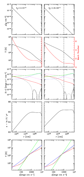
Figure 1.— Structure of 1-D accretion flow in run 1D256C (left column, $f_{X}=1\times 10^{-2}$) and 1D256D (right column, $f_{X}=1.5\times 10^{-2}$). Each panel is a snapshot taken at t=20 Myr. Panels from top to bottom show: density, temperature with Mach number (Mach number scale is on the right hand side), heating/cooling rates, and entropy S. The dashed vertical line in top panels marks the position of the sonic point. In panel with heating/cooling rates the black solid line is a net heating/cooling and color lines indicate particular physical process included in the calculations: Compton heating (red line), photoionization heating (green line), bremsstrahlung cooling (magenta-line), cooling through line emission (blue-line). The bottom panels display the gas temperature as a function of photoionization parameter; color lines indicate gas in radiative equilibrium (red), constant pressure conditions (blue) and free-fall compression (green).

Inspecting the bottom panels in Figure 1, one can suspect the gas is in the middle section of the computational domain to be thermally unstable because the slope of the $T-\xi$ relation (in the log-log scale) is larger than 1. Notice also that in both solutions the entropy is a non-monotonic function of radius. The regions where the entropy decreases with increasing radius correspond to the regions where there is net heating and the Schwarzschild criterion indicates convective instability at these radii. We therefore conclude that both solutions could be unstable. We first check more formally the thermal stability of our solutions.

4.2. Thermal Stability of Steady Accretion Flows

The linear analysis of the growth of thermal modes under the radiative equilibrium conditions (${\mathcal{L}}(\rho_{0},T_{0})=0$) has been examined in detail by Field (1965) (see Appendix for basic definitions). In Figure 2, in the top panels (left and right column correspond again to model 1D256C and D), we show the radial profiles of various mode timescales. The timescales, $\tau=1/n$, are calculated using definitions A2 and A3. The growth timescale of short wavelength, isobaric condensations $\tau_{TI}=-1/N_{p}$ is positive (thermally unstable zone marked with the dotted line) in a limited radial range between about 10 and 100 pc. The location of the thermally unstable zone depends on the central source luminosity, and it moves outward with increasing $f_{X}$. The long wavelength, isochoric perturbations are damped, at all radii, on timescales of $\tau_{v}=-1/N_{v}$ (faster than TI development). The short wavelength nearly adiabatic, acoustic waves are damped as well, and $\tau_{ac}=-2/(N_{v}-N_{p})$. In Figure 2, the dashed line is the accretion timescale $\tau_{acc}=r/v$. Within the thermally unstable zone, $\tau_{TI}$ is short in comparison to $\tau_{acc}$, in both models.

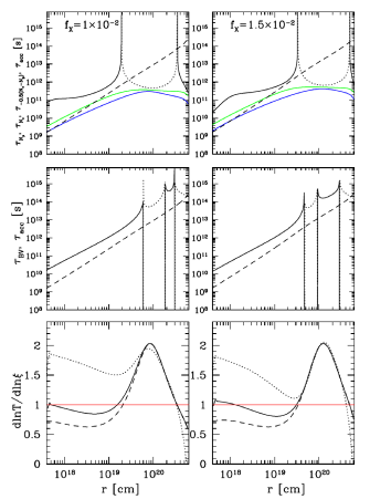
Figure 2.— Left and right panels correspond, respectively to runs 1D256 C and D. Top panels show the instability growth rates in comparison to the accretion time scale ($\tau_{acc}=r/v$, dashed line). The time scale for the short wavelength isobaric mode growth is displayed as the dotted line while the damping rate as solid line ($\tau_{N_{p}}$). Other two lines show the long-wavelength isochoric mode damping rate $\tau_{N_{v}}$ (heavy line) and the effective acoustic waves damping time scale $\tau_{N_{v}}$ (light line). Middle panel: The dashed line is $\tau_{acc}$ and solid line is $t_{BV}=1/\omega_{BV}$, where $\omega_{BV}^{2}>0$ is the ${\rm Brunt-V\ddot{a}is\ddot{a}l\ddot{a}}$ oscillation frequency for a spherical system. Solid lines show the regions which are unstable convectivelly. The dotted line indicates region where $\omega_{BV}^{2}<0$ and oscillations are possible. Bottom panels: the derivative $d\ln T/d\ln\xi$ as a function of radius is shown as a solid line. $(d\ln T/d\ln\xi)_{ad}$ for an adiabatic inflow is marked as dotted line, and dashed line is the same derivative for radiative equilibrium conditions. Horizontal one indicates slope of 1.

Balbus (1986), Balbus & Soker (1989), Mathews & Bregman (1978), (and also Krolik & London 1983) extended the analysis by Field (1965) to spherical systems with gravity, in more general case when initially the gas is not in the radiative equilibrium. Their approximate solution gives the formula for linear evolution of the short wavelength, isobaric, radial perturbation as it moves with smooth background accretion flow (Equation 23 in Balbus 1986 or Equation 4.12 in Balbus & Soker 1989). Since the two presented solutions are close to radiative equilibrium, the approximate formula for the growth of a comoving perturbation given by Balbus & Soker (1989) reduces to

$$\delta(r)=\frac{\delta\rho}{\rho}=\delta_{s}\exp\left(\int_{r_{s}}^{r_{f}}-\frac{N_{p}(r^{\prime})}{v(r^{\prime})}dr^{\prime}\right),$$ (12)

where $N_{p}(r^{\prime})$ is a locally computed growth rate of a short wavelength, isobaric perturbation as defined in the Appendix or Field (1965), $r^{\prime}$ is radius where $N_{p}(r^{\prime})<0$, and $\delta_{s}$ is an initial amplitude of a perturbation at some starting radius $r=r_{s}$. Using Equation 12, the isobaric perturbation amplification factors are $\delta/\delta_{s}\approx 10^{10},10^{16},10^{19}$ and $10^{33}$, for models 1D256A, B, C, and D, respectively. Notice that these amplification factors are calculated for the asymptotic, maximum physically allowed growth rate, $n=-N_{p}$, which might not be numerically resolved.

To quantify the role of TI in our simulations we ought to address the following question. What is the minimum amplitude and wavelength of a perturbation in our computer models? The smallest amplitude variability is due to machine precision errors, $\epsilon_{machine}\approx 10^{-15}$ (for a double float computations). The typical $\lambda$ of these numerical fluctuations are of the order of the numerical resolution, $\Delta r_{i}$. The discretization of the computational domain affects the TI growth rates in our models in two ways: (1) the numerical grid refinement limits the size of the smallest fragmentation that can be captured; (2) the rate at which the condensation grows in the numerical simulations depends on number of points resolving a condensation. As shown in Appendix the perturbation of a given $\lambda$ has to be resolved by 20, or more, grid points. A wavelength $\lambda_{0}$ for which $n=-0.9973\times N_{p}$ is shown in Figure 3 together with $\Delta r_{i}$ as a function of radius for models with $N_{r}$=256, 512, 1024, 2048, and, 4096 grid points. In low resolution models we marginally resolve $\lambda_{0}$. We therefore expect the TI fragmentations to grow slower than theoretical estimates. Reduction of the growth rate due to these numerical effects even by a factor of a few is enough to suppress variability because of the strong exponential dependence.

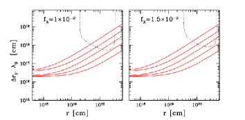
Figure 3.— Grid spacing (red lines) in models with $N_{r}$=256, 512, 1024, 2048, and 4096 points and $\lambda_{0}$ (black, dotted line) as a function of radius in models 1D256 C (left panel) and D (right panel).

Thermal mode evolution depends not only on the numerical effects but also other processes affecting the flow. Figure 4 shows the comparison of time scales of physical processes involved: the compression due to geometry of the inflow and stretching due to accretion dynamics. We expect that any eventual condensation formed from the smooth background which leaves the thermally unstable zone, would accrete with supersonic background velocity. From the continuity equation, the co-moving density evolution is a balance of two terms $(1/\rho)(D\rho/Dt)=-2v/r-\partial v/\partial r$, i.e., the compression and tidal stretching. The amplitude of condensation grows in regions where there is compression due to geometry and decreases in regions where fluid undergoes acceleration - it stretches the perturbation. In the models 1D256D and C interior of the TI zone, the evolution of the perturbation is dominated by compression because the compression time scale is the shortest.

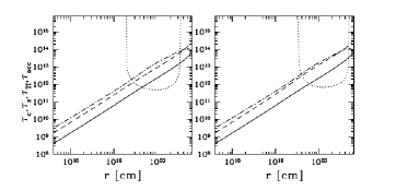
Figure 4.— Time scales in 1-D, stationary models 1D256 C (left panel) and 1D256 D (right panel): accretion time scale ($\tau_{acc}$, dashed line), compression time scale ($\tau_{c}$, solid line), tidal stretching time scale ($\tau_{s}$, dotted-dashed line), and condensation growth time scale ($\tau_{TI}$, dotted line).

4.3. Convective Stability of Steady Accretion Flows

In this subsection, we examine in more detail convective stability of our solutions. In Figure 2, (middle panels), we compare the accretion time scale $\tau_{acc}$ and the ${\rm Brunt-V\ddot{a}is\ddot{a}l\ddot{a}}$ time scale $\tau_{BV}=\frac{1}{\omega_{BV}}$ associated with the development of convection. The frequency $\omega_{BV}$ is defined as $\omega_{BV}^{2}\equiv(-\frac{1}{\rho}\frac{\partial P}{\partial r})\frac{\partial\ln S}{dr}$. The convectivelly unstable regions are marked as solid lines ($\omega_{BV}^{2}>0$). The convectivelly unstable zones overlap with the thermally unstable zones. Since $\tau_{acc}\ll\tau_{BV}$ convective motions might not develop, at least at the linear stage of the development of TI.

In the bottom panels of Figure 2 we show the logarithmic derivatives of $d\ln T/d\ln\xi$ that could be used to graphically assess the stability of the flow. This can be done by comparing the derivatives (the slopes of the $lnT-\ln\xi$ relation) for three cases: model data (solid line where $T$ and $\xi$ are taken directly from the simulations), purely adiabatic inflow (dotted line, assuming that the velocity profile is same as in the numerical solution), and radiative equilibrium conditions (dashed line). In particular, the regions where the solid line is above the red line correspond to the potentially TI zones. The regions where the dotted line is below the solid line correspond with the zone where the flow is potentially convectivelly unstable. The conclusion regarding the flow stability is consistent with the conclusion reached by analyzing the time scales shown in the top and middle panels of Fig. 2.

4.4. Other Physical Consequences of Radiative Heating and Cooling - obscuration effects

Figure 5.— Fraction of central illuminating source radiative energy intrinsically absorbed (upper panels) and emitted (bottom panels) by gas per second as a function of time. We show the steady state solutions $1D256C$ and $1D256D$ in left and right panels, respectively. Solid lines show the net absorption/emission and dashed lines indicate the intrinsic absorption and emission.

The growth of the thermal instability leads to the development of a dense cold clouds (shells in 1-D models; e.g. variable phase in model 1D256D). The enhanced absorption in the dense condensations may make them optically thick. Here we check if the time-dependent models are self-consistent with our optically thin assumption. Figure 5 shows the amount of energy absorbed and emitted by the gas (heating and cooling rates integrated over a volume at each time moment) in comparison to the luminosity of the central source in models 1D256C and D. Solid lines show the net rate of the energy exchange between radiation and matter (cooling function ${\mathcal{L}}$ integrated over the simulation volume) while dashed lines indicate the intrinsic absorption and emission (heating and cooling terms used in ${\mathcal{L}}$ are integrated independently). The net heating-cooling rate is mostly much lower than unity reflecting the fact that in the steady state the gas is nearly in a radiative equilibrium. During a variable phase (part of model 1-D256D) the energy absorbed by the accretion flow (black solid line) becomes comparable to the X-ray luminosity of the central black hole. During this variable phase the optical thickness of accreting shells can increase up to $\tau_{X,sc}\approx 20$ where the majority contribution to opacity is due to photoionization absorption. The average optical thickness increases in models with higher resolution indicating that the flow is more variable and condensations are denser. This increase in optical depth is related to shells condensating much faster in runs with higher resolutions. The dense condensations falling towards the center could reduce the radiation flux in the accretion flow at larger distances. It is beyond the scope of the present paper to investigate the dependence of the flow dynamics on the optical thickness effects and we leave it to the future study.

Significant X-ray absorption is related also to transfer of momentum from radiation field to the gas. To estimate the importance of the momentum exchange between radiation and matter, one can compute a relative radiation force:

$$f_{force}\equiv\frac{\sigma_{sc}+\sigma_{X}}{\sigma_{TH}}f_{X}$$ (13)

where $\sigma_{X}$ is the energy averaged X-ray cross-section. The momentum transfer is significant when $f_{force}>1$. Using our expression for the heating function due to X-ray photoionization $\sigma_{X}/\sigma_{TH}=H_{X}/n/F_{X}=2.85\times 10^{4}\xi^{-3/4}T^{-1/2}$ (see § 2). Even for a dense cold shell $f_{force}$ is at most 0.1 (in case when $\tau_{max}\approx 60$). Therefore radiation force is not likely to directly launch an outflow. However, the situation may change when optical effects are taken into account.

4.5. $\dot{M}$ Evolution

We end our presentation of 1-D results with a few comments on the time evolution of the mass accretion rate, $\dot{M}$. Figure 6 displays $\dot{M}$ vs time measured for all of our 1-D models. One can divide the solutions into two subcategories: steady and unsteady where $\dot{M}$ varies from small fluctuations to large changes. For a given $f_{X}$, the time behavior of the solution depends on the resolution, due to effects described above. In the variable models a fraction of the accretion proceeds in a form of a cold phase defined as all gas with $T<10^{5}$ K. Column 6 in Table 1 shows the ratio of cold to hot mass accretion rates, $\chi$, computed by averaging $\dot{M}^{\prime}s$ over the radius and simulation time. We average $\dot{M}^{\prime}s$ over $r<100$ pc because the cadence of our data dumps is comparable to the dynamical time scale at 100 pc. The larger the luminosity the more matter is accreted via the cold phase. However, the maximum value of $\chi$ is of the order of a few, so the dominance of the cold gas is not too strong.

Figure 6.— Mass accretion rate in 1-D solutions for $f_{X}=0.0005,0.08,0.01$, and $0.015$. Different colors shows $\dot{M}$ for various number of grid points: $N_{r}$=256 (blue), 512 (red), 1024 (green), 2048 (magenta), 4096 (black). 

Model ID	$f_{X}$	$N_{r}$	$N_{\theta}$	$t_{f}$	$\langle\dot{M}\rangle$	$\langle f_{Vol}\rangle_{t}$	$\langle\chi\rangle_{r,t}$	$\langle\tau_{X,sc}\rangle_{\theta,t}$	Max($\tau_{X,sc}$)	final state
				[Myr]	${\rm[M_{\odot}\,yr^{-1}]}$
2D256x64A	$5\times 10^{-4}$	256	64	20	2.0	$1\times 10^{-6}$	0	0.45	0.46	smooth
2D256x64B	$8\times 10^{-3}$	256	64	15.4	2.04	$1\times 10^{-6}$	$10^{-6}$	0.1	0.99	smooth
2D512x128B	$8\times 10^{-3}$	512	128	20	1.95	$1\times 10^{-4}$	0.02	0.11	4.7	clouds
2D1024x256B	$8\times 10^{-3}$	1024	256	1.83	1.84	$1.5\times 10^{-3}$	0.39	0.19	24.	clouds
2D256x64C	$1\times 10^{-2}$	256	64	11.8	1.94	$7\times 10{-5}$	0.15	0.11	2.5	smooth
2D512x128C	$1\times 10^{-2}$	512	128	20	1.88	$5\times 10^{-4}$	0.09	0.13	17.3	clouds
2D1024x256C	$1\times 10^{-2}$	1024	256	1.12	1.95	$4\times 10^{-3}$	0.5	0.24	70	clouds
2D256x64D	$1.5\times 10^{-2}$	256	64	12	1.57	$5\times 10^{-3}$	0.3	0.14	37.8	clouds
2D512x128D	$1.5\times 10^{-2}$	512	128	11	1.6	$3\times 10^{-3}$	0.43	0.12	13.2	outflow,filaments

Table 2 List of 2-D solutions. Columns from left to right are: model ID, $f_{X}$ - dimensionless luminosity, $N_{r},N_{\theta}$ - numerical resolution in radial and tangential direction, $t_{f}$ - final time of the simulation, $\langle\dot{M}\rangle_{t}$ - time averaged mass accretion rate, $\langle f_{Vol}\rangle_{t}$ - time averaged volume filling factor, $\chi$ - a ratio of cold to hot mass accretion rate averaged over radii less than $10^{20}$ cm and simulation time, (cold phase is any gas with temperature $T<10^{5}$ K), $\langle\tau_{X,sc}\rangle_{\theta,t}$ - angle and time averaged optical depth, Max($\tau_{X,sc}$) - maximum optical depth recorded during the simulation, and comments. In the beginning of all runs the accretion flow becomes unsteady due to randomly seeded perturbations, at $t_{f}$ the flow either returns to the original, unperturbed, smooth state (globally stable solutions), or remains unsteady with coexisting, two phase medium (cold clouds embedded in a warm gas). Only in one model a large scale outflow forms (model 2D512x128D).

5. Results: 2-D models

5.1. Seeding the TI

To investigate the growth of instabilities in 2-D, we solve eqs. 1, 2, 3, for the same parameters $M_{BH}$ and $f_{X}$ as in § 4, but on a 2-D, axisymmetric grid with $\theta$ angle changing from 0 to $90\deg$. We use three sets of numerical resolutions described in § 3. To set initial conditions in axisymmetric models, we copy the solutions found in 1-D models onto the 2-D grid. In case of time-independent 1-D models, our starting point, is the data from $t=t_{f}$. We checked, for example, the runs 2D256x64 A, B, C, and D (which are 2-D version of models 1D256A, B, C, and, D) are time-independent at all times as expected. In case of higher resolution models, for which the 1-D, steady state models do not exist we adopt a quasi-stationary data from the 1-D run early evolution (at $t$ of a fraction of a Myr), during which the flow is already relaxed from its initial conditions but the TI fluctuations are not yet developed. Models which are time varying in 1-D, in 2-D develop dynamically evolving spherical shells, as expected, also indicating that our numerical code keeps a symmetry in higher dimensions.

To break the symmetry in 2-D models, we perturb the smooth solutions adopted as initial conditions. The perturbation of a smooth flow is seeded everywhere and has a small amplitude randomly chosen from a uniform distribution. The new density at each point is $\rho=\rho_{0}(1+Amp*rand)$, where $rand$ is a random number $rand\in(-1,1)$ and maximum amplitude $Amp=10^{-3}$. To seed the isobaric, divergence free fluctuations other (than $\rho$) hydrodynamical variables are left unchanged. The amplitude magnitude $Amp$ is chosen to be much higher in comparison to $\epsilon_{machine}$, in order to investigate the development and evolution of strongly non-linear TI on relatively short time scales, starting directly from a linear regime. The list of all perturbed, 2-D models is given in Table 2.

5.2. Formation of Clouds, Filaments, & Rising Bubbles

For luminosities $L_{X}<0.015~{}L_{Edd}$, the 2-D models show similar properties to the 1-D models. The gas is thermally and convectivelly unstable within the computational domain, and we observe that very tiny fluctuations in an initially smooth, spherically symmetric, accretion flow, grow first linearly and then non-linearly. Since the symmetry is broken the cold phase of accretion forms many small clouds. For $L_{X}=0.015~{}L_{Edd}$ or higher, the cold clouds continue to accrete but in some regions a hot phase of the gas starts to move outward.

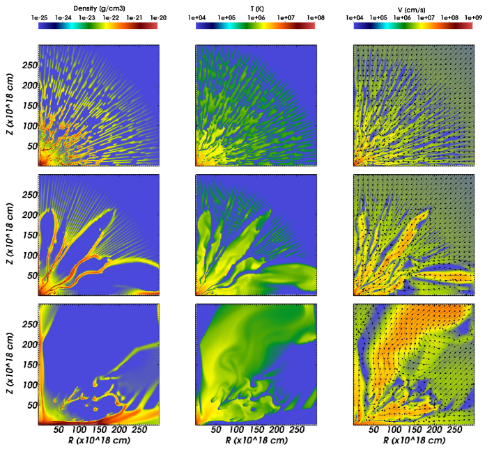
Figure 7.— Density, temperature, velocity magnitude with velocity direction (left, middle, and right column, respectively) in model 2D512x128D at t=3, 6 and 12 Myr (upper, middle, and bottom rows, respectively). Each panel show inner parts of the flow at $r\leq 100$ pc.

In Figure 7, we show three snapshots of representative 2-D model 2D512x128D at various times (t = 3, 6 and 11.8 Myrs). This model has the best resolution and the highest luminosity for which we are able to start the evolution from nearly steady state conditions. Columns from left to right show density, temperature, and total gas velocity overplotted with the arrows indicating the direction of flow. Initially (at t=3 Myr) the smooth accretion flow fragments into many clouds, which are randomly distributed in space. The cooler, denser regions are embedded in a warm background medium. The colder clouds are stretched in the radial direction and they have varying sizes. This initial phase of the evolution is common for all models in Table 2.

The phase where many cold clouds accrete along with the warm background inflow is transient. At a later stage (t=6 Myr, middle panels), model 2D512x128D shows a systematic outflow in form of rising, hot bubbles. The outflow is caused by the pressure imbalance between the cold and hot matter and buoyancy forces. The hot bubbles expand at speeds of a few hundreds km/s. Despite of the outflow, the accretion is still possible. During the rising bubble phase, the smaller clouds merge and sink towards the inner boundary as streams/filaments. However, even this phase is relatively short-lived. Bottom panels in Figure 7 show the later phase of evolution when some of the filaments occasionally break into many clouds (this process takes place between 10 and 50 pc). These ’second generation’ clouds occasionally flow out together with a hot bubble. Along the X-axis, we see an inflow of a dense filament.

To quantify the properties of clumpy accretion flow, we measure the volume filling factor of a cold gas $f_{vol}$, defined as:

$$f_{Vol}=V_{cloud}/V_{tot}$$ (14)

where $V_{cloud}$ is the volume occupied by gas of $T<10^{5}$ K, and $V_{tot}$ is the total volume of the computational domain. In model 2D512x128D, the time-averaged $f_{Vol}$ is $\langle f_{Vol}\rangle=3\times 10^{-3}$. The time evolution of $f_{vol}$ within 60 pc is shown in Figure 8 (black, solid line). The $f_{Vol}$ is variable and at the moment of the outflow formation, $f_{Vol}$ suddenly decreases by a factor of about 4. For comparison $f_{Vol}$ calculated during run 2D256x64D is also shown (blue, dashed line). Run 2D256x64D has the same physical parameters as 2D512x128D, however, no outflow forms. In the latter case, $f_{vol}$ is less variable and larger. In Table 2, we gather the time averaged $\langle f_{Vol}\rangle$ for all 2-D solutions. Measuring $f_{Vol}$ allows to quantify whether the perturbed accretion flow returns to its original, smooth state. We find that this happens when the $\langle f_{Vol}\rangle\approx 10^{-5}$ or smaller (models 2D256x64A, B, and C).

Figure 8.— Evolution of the volume filling factor $f_{vol}$ in model 2D512x128D (black, solid line) and 2D256x64D (dashed, blue line).

5.3. $\dot{M}$ Evolution

Figure 9 presents $\dot{M}$ through the inner boundary measured as a function of time. In most cases (except model 2D256x64A), $\dot{M}$ becomes stochastic instantly with spikes corresponding to the accretion of colder but denser clouds similar to those in Figure 7 (upper panels). Similar to 1-D models, one can divide the solution into two types: steady and unsteady state. In the latter, $\dot{M}$ fluctuates on various levels depending on $f_{X}$.

Figure 9.— Mass accretion rate in 2-D models with initially seeded random perturbations. Various colors code the $\dot{M}$ in models calculated with various grid resolutions: 2D256x64 (blue), 512x128 (red), 1024x256 (green). Results are sensitive to the resolution same as in 1-D models. 

Table 2 lists several characteristics of our 2-D simulations, for example, the ratio $\langle\chi\rangle_{t}$ averaged over time. In 2-D models this variable is smaller in comparison to 1-D due to geometry of the clouds. The maximum value of $\langle\chi\rangle_{t}$ is less than unity. This indicates that multi-dimensional effects (specifically development of convection) promote hot phases accretions. We plan to investigate this issue in future by carring out 3-D simulations.

We find that a large scale outflow forms only in run 2D512x128D. But even in this case, the $\dot{M}$ is not significantly affected by the outflow. Figure 10 shows the mass outflow rate (dashed line), inflow rate (dotted lines) and total mass flow rate (solid line) as a function of radius. The same types of lines show $\dot{M}$ for various times of the simulation (t=3, 6 and 11.8 Myr, green, blue and black lines, respectively) and they are averaged over $\theta$ angle. The rising bubble originates at about 10 pc in this case. We anticipate that large scale outflow are common and significant for high luminosity cases (i.e., for $f_{X}>0.02$).

Figure 10.— Model 2D512x128D: In-, out- and total mass flow rate as a function of radius for three time moments shown in Figure 7 (green, blue, and black correspond to t=3, 6 and 11.8 Myr). The solid lines mark the inflow rates while the dashed line - outflow rate. The dotted line is the total mass flow. 

5.4. Obscuration Effects

Here we again check whether the cloud opacity might affect our results. The averaged optical thickness of the filaments and clouds is similar (see Table 2, columns 8 and 9). In Figure 11 we show how much energy is absorbed and emitted in run 2D512x128D during the evolution. The figure shows the intrinsic absorption and emission integrated over the entire computational domain. We next calculate $\langle\tau_{X,cs}\rangle$ (optical thickness due to absorption, averaged over angles and times) and maximum value of $\tau_{X,cs}$ that occurred during the evolution. In case of the largest optical depth of $\tau\approx 70$ (in run 2D1024x256C) the radiation force coefficient from Equation 13: $f_{force}\approx 0.2$ which, as in 1-D models, is small but might not be negligible. Therefore, we are planning to explore the effects of optical depth in a follow-up paper.

Figure 11.— Fraction of central illuminating source radiative energy intrinsically absorbed (upper panel) and emitted (bottom panel) by gas per second as a function of time in models 2D512x128 (red, solid line) and 2D256x64D (blue, dotted line).

6. Summary and Discussions

In this work we show the evolution of thermal instabilities in gas accreting onto a supermassive black hole in an AGN. A simplified assumptions made in this work, in particular constant X-ray luminosity emitted near the central SMBH regardless of the $\dot{M}$, allows to follow the development of TI from the linear to strongly non-linear and dynamical stage up to luminosities of $L\approx 1.5\times 10^{-2}~{}L_{Edd}$.

In our 1-D models the TI is seeded by numerical errors which might be non-isobaric and are initially under-resolved. In the initial phase, the TI growth rate is smaller than predicted by theory. The rate is affected by grid resolution which leads to the formation of cold clouds of various sizes and density contrasts. This is reflected in the mass accretion rate fluctuating at different amplitude and rate for the same physical conditions but different resolutions. One cannot avoid dealing with these numerical difficulties in the numerical models. Nevertheless, we find the under-resolved, 1-D models very useful in quick checking where the thermally unstable zone exists and what type of fluctuation could cause the smooth to turn into a two-phase medium. For given physical conditions, Figure 3 shows the wavelength $\lambda_{0}$ and Equation 12 gives the amplitude of an isobaric perturbation required to break the smooth flow into a two-phase, time-dependent model.

In 2-D models, although the models depend on the resolution effects same way as in 1-D setup, we can observe an outflow formation. The convectivelly unstable gas buoyantly rises and, as found in this work, controls the later evolution of the two-phase medium and mass accretion rate. Given a simple set up with minimum number of processes included, our models display the three major features needed to explain some of the AGN observations: cold inflow, hot outflow and cold, dense clouds which occasionally escape, advected with the hot wind. We show that an accretion flow at late, non-linear stages, thus most relevant to observations, are dominated by buoyancy instability not TI. This suggests that the numerical resolution might not have to be as high as that needed to capture the small scale TI modes and it is sufficient to capture significantly larger and slower buoyancy modes. We plan to check the consistency of the models with the observations by calculating the synthetic spectra, including emission and absorption lines based on our simulation following an approach like the one in Sim et al. (2012). Here, we only briefly comment on the main outflow properties and compare them some observations of outflows in Seyfert galaxies.

Space Telescope Imaging Spectrograph (STIS) on board the Hubble Space Telescope allows us to map the kinematics of the Narrow Line Regions in some nearby Seyfert Galaxies (e.g. for NGC 4151 Das et al. 2005; NGC 1068; Das et al. 2006; Mrk 3, Crenshaw et al. 2010; Mrk 573, Fischer et al. 2010; and Mrk 78, Fischer et al. 2011). Position-dependent spectra in [O III] $\lambda$ 5007 and $H_{\alpha}$ $\lambda$ 6563, and the measurements of the outflow velocity profiles show the following general trend: the outflow has a conical geometry and the [O III] emitting gas accelerates linearly up to some radius and then decelerates. The velocities typically reach up to about 1000 km/s and a turnover radius is on one hundred to a few hundred parsec scales.

To compare our results with the observations, Figure 12 shows the radial velocity of hot and cold gas versus the radius at t=11.8 Myr for model 2D512x128D (the data correspond to a snapshot shown in the right panels in Figure 7). We reiterate that our model is quite simplified (e.g., no gas rotation) and the outer radius is relatively small (i.e., 200 pc). Therefore, our comparison is only illustrative.

We find that the hot outflow originates at around 10 pc and accelerates up to about $v_{max}\approx 200{\rm km/s}$, which is comparable to the escape velocity from 10 pc, $v_{esc}=314~{}{\rm km/s}$. At larger distances, r = 100-200 pc, we see a signature of deceleration which is consistent with the observations of Seyferts outflows. We note that the geometry of the simulated flow is affected by our treatment of the boundaries of the computational domain, specifically along the pole and the equator we use reflection boundary conditions (see § 3).

The scatter plot also indicates that the cold clouds appear at about 20-80 pc. Their maximum velocity is about $v_{max}=100$ km/s, which is smaller than the velocity of the hot outflow. The plot does not show a clear indication of a linear acceleration of the outflowing cold gas. However, it is possible that the cold clouds, seen in this snapshot, will continue to be dragged by the hot outflow and eventually will reach higher velocities.

We also measured the column density of the hot and cold gas for the same, representative, snapshot at t=11.8 Myrs. The typical column densities vary with the observer inclination, $N_{H}=5\times 10^{22}-10^{24}\,{\rm cm^{2}}$ for gas $T>10^{5}$ K, and $N_{H}=10^{20}-10^{23}\,{\rm cm^{2}}$ for gas with $T<10^{5}$ K. This is roughly consistent with column densities estimated from observations of AGN (e.g. for NGC 1068 $N_{H}=10^{19}-10^{21}\,{\rm cm^{2}}$, Das et al. 2007 and references therein).

Our results are similar in many respects, to the previous findings presented in Barai et al. (2012), i.e. the accretion evolution depends on $f_{X}$ luminosity; we also observe clouds, filaments and outflow. The outflow appears at $f_{X}=0.015$ which is consistent with $f_{X}=0.02$ found by Barai et al. (2012). Here, we are able to calculate models for about 10 times longer in comparison to 3-D SPH models. We confirm the previous results that the cold phase of accretion rate can be only a few times larger in comparison to the hot one.

Similar models has been investigated in the past by e.g. Krolik & London (1983). Our work is on one hand a simplified and on the other hand an extended version of these previous works. The key extention here is that our new results cover the non-linear phase of the evolution. There are two new conclusions added by our analysis to the previous investigations. The 2-D models with outflows are possibly governed by other than TI instabilities mainly convection. Another non-linear effects found in our 1-D and 2-D models is that the fragmentation of the flow makes it optically thick for photoionization. Further investigation of shadowing effects is required.

Some sub-resolution models of AGN feedback in galaxy formation (Di Matteo et al. 2008; Dubois et al. 2010; Lusso & Ciotti 2011) assume that BH accretion is dominated by an unresolved cold phase, in order to boost up the accretion rate obtained in simulations. Our results indicate that the cold phase accretion is unlikely dominant as even in well-developed and well- resolved multi-phase cases, the accretion is typically dominated by a hot phase. However, we note that the cold phase of our solution might be an upper branch of some more complicated multi-phase medium (i.e., a mixture of molecular, atomic and dusty gas).

This work was intentionally focused on a very limited number of processes and effects. Its results suggest that the future work should include more self-consistent approach not only with shadowing effects but also with the radiation force. Our next step would be to investigate the non-axisymmetric effects via fully 3-D simulations. The latter is challenging and one may not be able to see very fine details of the gas dynamics as in 2-D models due to resolution effects.

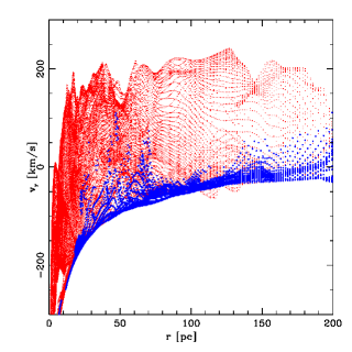
Figure 12.— Scatter plot of radial velocity of hot ($T>10^{5}K$, smaller red symbols) and cold ($T<10^{5}K$, larger blue symbols) phase of the flow in model 2D512x128D at t=11.8 Myr (model shown in right panels in Figure 7).

Appendix A Growth rate of a condensation mode in a uniform medium -code tests

Field (1965) formulated a linear stability analysis of a gas in thermal and dynamical equilibrium. Here, we briefly recall his most important, for our analysis, equations. We disregard the thermal conduction effects. The dispersion relation derived from linearized local fluid equations with heating/cooling described by ${\mathcal{L}}$ function and perturbed by a periodic, small amplitude wave given by $\exp(nt+ikx)$, is:

$$n^{3}+N_{v}n^{2}+k^{2}c_{s}^{2}n+N_{p}k^{2}c_{s}^{2}=0$$ (A1)

where $k$ is the perturbation wave number ($k=2\pi/\lambda$) and functions $N_{p}$ and $N_{v}$ are defined as

$$N_{p}\equiv\left.\frac{1}{c_{p}}\left(\frac{\partial{\mathcal{L}}}{\partial T}\right)\right|_{P}$$ (A2)

and

$$N_{v}\equiv\left.\frac{1}{c_{v}}\left(\frac{\partial{\mathcal{L}}}{\partial T}\right)\right|_{\rho}$$ (A3)

with $c_{p}$ and $c_{v}$ being the specific heats under constant pressure and constant volume conditions, respectively, and $T$ is the gas temperature. Vertical line means that the derivative is taken under constant thermodynamical variable condition. Dispersion Equation A1 has three roots. In a short wavelength regime ($\lambda\ll 2\pi N_{p}/c_{s}$), two, complex roots correspond to two conjunct nearly adiabatic sound waves and third, real one is an isobaric condensation mode (the gas density and temperature change in anti-phase so that the pressure remains constant). The sign of the real part of the root gives the stability criterion. The sound wave will grow if $\left.\partial{\mathcal{L}}/\partial T\right|_{S}<0$ (known as Parker’s criterion, Parker 1953). The condensation mode will grow if $\left.\partial{\mathcal{L}}/\partial T\right|_{P}<0$ (Field’s criterion). In a short wavelength limit, the growth rates asymptote to $n=-0.5(N_{v}-N_{p})$ (for sound waves) and $n=-N_{p}$ (for condensation modes). Isochoric modes ($n\rightarrow-N_{v}$) and effective acoustic waves are eigen modes of long wavelengths perturbations. The perturbation growth/damp time scale is $\tau_{TI}=1/n$.

We use the above Field (1965) theory to show that our numerical scheme for solving the modified energy conservation equation (Equation 3) together with two other fluid dynamics equations is accurate. The test calculations are carried out in 1-D Cartesian coordinates within $x\in(0,L)$ range where L is the size of the computational domain in dimensionless units. The boundary conditions for all variables are periodic. In an unperturbed state, the gas density ($\rho_{0}=1$) and internal energy density ($e_{0}=1$) are constant in the entire computational domain. The velocity of gas is set to zero. We assume that the gas is heated by an external source of radiation and cools due to free-free transitions. The test cooling function is simple:

$${\mathcal{L}}=C\rho T^{1/2}-H$$ (A4)

The normalization constants $H$ (for heating) and $C$ (for cooling) are set so that in the unperturbed state the gas is in radiative equilibrium i.e. ${\mathcal{L}}(\rho_{0},e_{0})=0$. In this test the functions $N_{p}$ and $N_{v}$ have explicit, analytical forms

$$N_{p}\equiv\left.\frac{1}{c_{p}}\left(\frac{\partial{\mathcal{L}}}{\partial T}\right)\right|_{P}\equiv\frac{1}{c_{p}}\left(\left.\frac{\partial{\mathcal{L}}}{\partial T}\right|_{\rho}-\frac{\rho}{T}\left.\frac{\partial{\mathcal{L}}}{\partial\rho}\right|_{T}\right)=-\frac{1}{2c_{p}}C\rho_{0}T_{0}^{-1/2}$$ (A5)

and

$$N_{v}\equiv\left.\frac{1}{c_{v}}\left(\frac{\partial{\mathcal{L}}}{\partial T}\right)\right|_{\rho}=\frac{1}{2c_{v}}C\rho_{0}T_{0}^{-1/2}=-\gamma N_{p}.$$ (A6)

The numerical values of limiting growth/damp rates are $N_{p}=-0.04$, and $N_{v}=0.067$, while the speed of sound is: $c_{s}^{2}=1.11$ ($\gamma=5/3$). The domain sound crossing time is much shorter than the perturbation growth time scale which allows to keep the constant pressure.

Our numerical scheme implemented into ZEUS-MP code correctly reproduces the expected growth rates of small amplitude perturbation of the uniform medium. The perturbation is an eigen mode of TI, and its properties depend on the assumed $\lambda$. Eigen modes are realized by first applying a cosine perturbation to the gas density $\rho=\rho_{0}+A\rho_{0}\cos(kx)$ and calculating profiles of $e$ and $v$ from e.g. Equations 11 and 14 in (Field, 1965), for a given $k$ and corresponding theoretical value of $n$ (given by Equation A1). Next we measure how fast the perturbation grows while it is in the linear regime. Figure 13 (left panel), shows the analytical solution of the theoretical dispersion relation $n(\lambda)$ (solid line, third root of Equation A1), and the numerical growth rates calculated with ZEUS-MP (points). For very short $\lambda$’s the eigen mode of this root is converging to the isobaric condensation mode and grows at $n=-N_{p}$ rate, as expected. The long $\lambda$ modes grow slower in comparison to the very short $\lambda$ condensations, as predicted by theory. For relatively large $\lambda$, the third root changes into an effective acoustic wave, it becomes complex with the real part negative meaning that the waves are damped (see Shu 1992, Equation 41 in the Problem Set No 3).

Figure 13.— Left panel: Analytical (solid line; third root of Equation A1) and numerical (points; calculated with ZEUS-MP) linear growth rates of an eigen mode with wavelength $\lambda$. The initial amplitude of a perturbation is $A=10^{-3}$. The numerical solution uses $N_{x}=64$ grid points. Right panel: The condensation mode (density profile) with $\lambda=0.1L$ shown at t=10 T (where T here is a sound crossing time over the computational domain $L=1$) when it is resolved by 4, 8 and 16 points. The dotted line shows the very high resolution of 1600 points for which the condensation mode grows at the expected theoretical rate. Here the growth rate is as expected when resolved by at least with 16 points. For lower resolutions the condensations grow slower than one would expect.

In the second test, we measure the growth rate of a condensation mode that has a finite size (i.e. smaller than the domain length). We are interested in how many numerical grid points is required to resolve the correct $n$. We set $\lambda=0.1$ while $L=1$. Figure 13 (right panel) shows the same time snapshots of the growing condensation mode density, calculated with various numerical resolutions. Models with lower resolution evolve slower. When $\lambda$ resolved with 16 points it starts converging to the right solution. We conclude that about 20 or more grid points per $\lambda$ is required to resolve the isobaric condensation.

References

- Balbus (1986) Balbus, S. A. 1986, ApJ, 303, L79
- Balbus & Soker (1989) Balbus, S. A. & Soker, N. 1989, ApJ, 341, 611
- Barai et al. (2011) Barai, P., Proga, D., & Nagamine, K. 2011, MNRAS, 418, 591
- Barai et al. (2012) —. 2012, MNRAS, 3200
- Bisnovatyi-Kogan & Blinnikov (1980) Bisnovatyi-Kogan, G. S. & Blinnikov, S. I. 1980, MNRAS, 191, 711
- Blondin (1994) Blondin, J. M. 1994, ApJ, 435, 756
- Bondi (1952) Bondi, H. 1952, MNRAS, 112, 195
- Cowie et al. (1978) Cowie, L. L., Ostriker, J. P., & Stark, A. A. 1978, ApJ, 226, 1041
- Crenshaw et al. (2010) Crenshaw, D. M., Kraemer, S. B., Schmitt, H. R., Jaffé, Y. L., Deo, R. P., Collins, N. R., & Fischer, T. C. 2010, AJ, 139, 871
- Das et al. (2005) Das, V., Crenshaw, D. M., Hutchings, J. B., Deo, R. P., Kraemer, S. B., Gull, T. R., Kaiser, M. E., Nelson, C. H., & Weistrop, D. 2005, AJ, 130, 945
- Das et al. (2007) Das, V., Crenshaw, D. M., & Kraemer, S. B. 2007, ApJ, 656, 699
- Das et al. (2006) Das, V., Crenshaw, D. M., Kraemer, S. B., & Deo, R. P. 2006, AJ, 132, 620
- Di Matteo et al. (2008) Di Matteo, T., Colberg, J., Springel, V., Hernquist, L., & Sijacki, D. 2008, ApJ, 676, 33
- Di Matteo et al. (2012) Di Matteo, T., Khandai, N., DeGraf, C., Feng, Y., Croft, R. A. C., Lopez, J., & Springel, V. 2012, ApJ, 745, L29
- Dubois et al. (2010) Dubois, Y., Devriendt, J., Slyz, A., & Teyssier, R. 2010, MNRAS, 409, 985
- Field (1965) Field, G. B. 1965, ApJ, 142, 531
- Fischer et al. (2011) Fischer, T. C., Crenshaw, D. M., Kraemer, S. B., Schmitt, H. R., Mushotsky, R. F., & Dunn, J. P. 2011, ApJ, 727, 71
- Fischer et al. (2010) Fischer, T. C., Crenshaw, D. M., Kraemer, S. B., Schmitt, H. R., & Trippe, M. L. 2010, AJ, 140, 577
- Hayes et al. (2006) Hayes, J. C., Norman, M. L., Fiedler, R. A., Bordner, J. O., Li, P. S., Clark, S. E., ud-Doula, A., & Mac Low, M.-M. 2006, ApJS, 165, 188
- Janiuk et al. (2008) Janiuk, A., Proga, D., & Kurosawa, R. 2008, ApJ, 681, 58
- Kallman & Bautista (2001) Kallman, T. & Bautista, M. 2001, ApJS, 133, 221
- Krolik & London (1983) Krolik, J. H. & London, R. A. 1983, ApJ, 267, 18
- Kurosawa & Proga (2008) Kurosawa, R. & Proga, D. 2008, ApJ, 674, 97
- Kurosawa & Proga (2009a) —. 2009a, MNRAS, 397, 1791
- Kurosawa & Proga (2009b) —. 2009b, ApJ, 693, 1929
- Kurosawa et al. (2009) Kurosawa, R., Proga, D., & Nagamine, K. 2009, ApJ, 707, 823
- Lusso & Ciotti (2011) Lusso, E. & Ciotti, L. 2011, A&A, 525, A115
- Mathews & Bregman (1978) Mathews, W. G. & Bregman, J. N. 1978, ApJ, 224, 308
- Ostriker et al. (1976) Ostriker, J. P., Weaver, R., Yahil, A., & McCray, R. 1976, ApJ, 208, L61
- Parker (1953) Parker, E. N. 1953, ApJ, 117, 431
- Proga (2007) Proga, D. 2007, ApJ, 661, 693
- Proga et al. (2008) Proga, D., Ostriker, J. P., & Kurosawa, R. 2008, ApJ, 676, 101
- Proga et al. (2000) Proga, D., Stone, J. M., & Kallman, T. R. 2000, ApJ, 543, 686
- Shu (1992) Shu, F. H. 1992, Physics of Astrophysics, Vol. II (University Science Books)
- Sim et al. (2012) Sim, S. A., Proga, D., Kurosawa, R., Long, K. S., Miller, L., & Turner, T. J. 2012, ArXiv e-prints
- Springel (2005) Springel, V. 2005, MNRAS, 364, 1105
- Stellingwerf (1982) Stellingwerf, R. F. 1982, ApJ, 260, 768