On the Performance Limits of Map-Aware Localization

Abstract

Establishing bounds on the accuracy achievable by localization techniques represents a fundamental technical issue. Bounds on localization accuracy have been derived for cases in which the position of an agent is estimated on the basis of a set of observations and, possibly, of some a priori information related to them (e.g., information about anchor positions and properties of the communication channel). In this manuscript new bounds are derived under the assumption that the localization system is map-aware, i.e., it can benefit not only from the availability of observations, but also from the a priori knowledge provided by the map of the environment where it operates. Our results show that: a) map-aware estimation accuracy can be related to some features of the map (e.g., its shape and area) even though, in general, the relation is complicated; b) maps are really useful in the presence of some combination of low signal-to-noise ratios and specific geometrical features of the map (e.g., the size of obstructions); c) in most cases, there is no need of refined maps since additional details do not improve estimation accuracy.

I Introduction

Recently, localization systems have found widespread application, since they allow to develop a number of new services in both outdoor and indoor environments [1, 2]. Conventional localization systems acquire positional information from a set of observations; these are usually extracted from noisy wireless signals propagating in harsh environments. Unavoidably, this limits the accuracy that can be achieved by such systems.

Localization accuracy can certainly benefit from the availability of any form of a priori knowledge. In the technical literature, the sources of prior knowledge commonly exploited are represented by the positions of some specific nodes (called anchors) or by some characteristic of the communication channel; for instance in [3, 4, 5, 6] the impact of different factors (like non-line-of-sight, NLOS, propagation and network synchronization) on localization accuracy have been thoroughly analysed employing Cramer-Rao bounds (CRBs) and, when a priori knowledge is available, Bayesian Cramer-Rao bounds (BCRBs). In [7, 8, 9, 10] multipath propagation in ultra wide band (UWB) systems and its effects on time-of-arrival (TOA) estimation have been investigated by means of CRBs or BCRBs. In [11, 12, 13] CRBs and BCRBs for the analysis of cooperative localization techniques have been derived.

In recent times, however, some attention has been paid to the possibility of improving accuracy by endowing localization systems with map-awareness, i.e., with the knowledge of the map of the environment in which they operate. Specific examples of map-aware algorithms have been developed in [14, 15, 16, 17, 18], which propose the adoption of non-linear filtering techniques (namely, particle filtering and extended Kalman filtering) to embed map-based a priori information in navigation systems. This work evidences that this kind of information plays an important role in improving localization and navigation accuracy; however, the impact of map-awareness on the performance limits of localization systems is still an open problem. In fact, as far as we know, the technical literature dealing with the fundamental limits of localization accuracy [10, 12, 9, 13] has not considered this issue yet.

In this paper, novel accuracy bounds for map-aware localization systems are developed and their applications to specific environments are analysed. Specifically, the BCRB, the extended Zik-Zakai bound (EZZB) and the Weiss-Weinstein bound (WWB) for the above mentioned systems are derived. These bounds, which provide several novel insights into map-aware localization, have the following features:

1. they are characterized by different tightness/analytical complexity;

2. they can be evaluated for any map geometry and, in the cases of the BCRB and the EZZB, admit a closed form for rectangular maps;

3. they allow to a) identify map features (e.g., shape, area, etc.) influencing localization accuracy and b) quantify such an influence.

Then, such bounds are evaluated and compared for simple representative environments. Our results allow to assess the importance of map-awareness in localization systems in the presence of noisy observations. In particular, they evidence that:

1. maps should be expected to play a significant role at low signal-to-noise ratios (SNRs) and in the presence of obstructions;

2. in some cases simplified map models can be adopted for localization purposes, since map details have a negligible impact on estimation accuracy.

The manuscript is organized as follows. In Section II our reference scenario is illustrated and the map model is defined. Performance bounds for map-aware localization are derived and evaluated in specific scenarios in Sections III and IV, respectively. Finally, some conclusions are offered in Section V.

Notations: Matrices are denoted by upper-case bold letters, vectors by lower-case bold letters and scalar quantities by italic letters. The notation $\mathbb{E}_{\mathbf{r}}\left\{\cdot\right\}$ denotes expectation with respect to the random vector $\mathbf{r}$; $\operatorname{tr}\{\cdot\}$ denotes the trace of a square matrix; $\operatorname{diag}\{\cdot\}$ denotes a square matrix with the arguments on its main diagonal and zeros elsewhere; $[\cdot]_{i,l}$ is the element on the $i$-th row and $l$-th column of its argument. $\mathbf{I}_{N}$ denotes the $N\times N$ identity matrix; $\mathbf{A}\succeq\mathbf{B}$ means that the matrix $\mathbf{A}-\mathbf{B}$ is positive semi-definite. The probability density function (pdf) of the random vector $\mathbf{R}$ evaluated at the point $\mathbf{r}$ is denoted as $f(\mathbf{r})$, whereas $\mathcal{N}\left(\mathbf{r};\mathbf{m},\boldsymbol{\Sigma}\right)$ denotes the pdf of a Gaussian random vector having mean $\mathbf{m}$ and covariance matrix $\boldsymbol{\Sigma}$, evaluated at the point $\mathbf{r}$. $\mathbb{I}_{\mathcal{S}}(\mathbf{x})$ denotes the so called indicator function for the set $\mathcal{S}$ (it is equal to 1 when $\mathbf{x}\in\mathcal{S}$ and zero otherwise).

II Reference Scenario and Map Modelling

In the following we focus on the problem of localizing a single device, called agent, in a 2-D environment, i.e., of estimating its position $\mathbf{p}\triangleq[x,y]^{T}$, in the presence of the following information: a) a map representing the a priori knowledge about the environment in which the localization system operates; b) an observation vector $\mathbf{z}$ related to the true position $\mathbf{p}$ of the agent.

II-A Map Modelling

In a Bayesian framework the map of a given environment can be modelled for localization purposes as a pdf $f(\mathbf{p})$ of the random variable $\mathbf{p}$, representing the agent position. Such a pdf is characterized by a 2-D support $\mathcal{R}$ having a finite size and consisting of the set of points in the environment not occupied by obstructions (e.g., walls, buildings, etc). In the absence of other prior knowledge, a natural choice for $f(\mathbf{p})$ is a simple uniform model, i.e.,

$$f(\mathbf{p})=f(x,y)=\begin{cases}1/\mathcal{A_{R}}&\mathbf{p}\in\mathcal{R}\\ 0&\text{elsewhere}\end{cases}$$ (1)

where $\mathcal{A_{R}}$ denotes the area of $\mathcal{R}$. This model is referred to as uniform map in the following and is preferable to other, more detailed, prior models since it can be adopted when only basic knowledge of the environment is available (e.g., the floor plan of a building in indoor environments or satellite photos in outdoor environments). An alternative statistical model for maps, better suited to mathematical analysis in the BCRB case, is a “smoothed” version of (1); this is obtained modifying the uniform pdf in a narrow area around the edges of $\mathcal{R}$ in order to introduce a smooth transition to zero along the boundaries of its support. Note that the adoption of a smoothed uniform model leads to analytical results similar to those found with the uniform model if the transition region is small with respect to the size of $\mathcal{R}$.

As it will become clearer in the following, for a generic map, a detailed description of the structure of its support $\mathcal{R}$ should be provided to ease the formulation of the accuracy bounds referring to the map itself.

To begin, let us define, for each $(x,y)\in\mathbb{R}^{2}$, the sets $\mathcal{R}_{h}(y)\triangleq\left\{t|(t,y)\in\mathcal{R}\right\}$ and $\mathcal{R}_{v}(x)\triangleq\left\{t|(x,t)\in\mathcal{R}\right\}$ representing the intersection between $\mathcal{R}$ and an horizontal (h) and vertical (v) line identified by the abscissa $x$ and ordinate $y$, respectively. Then, let:

• $N_{h}(y)$ and $N_{v}(x)$ denote the number of connected components of $\mathcal{R}_{h}(y)$ and $\mathcal{R}_{v}(x)$, respectively;

• $\mathcal{N}_{h}^{o}(y)$ and $\mathcal{N}_{v}^{o}(x)$ denote the set of the odd values $\left\{1,3,...,2N_{h}(y)-1\right\}$ and $\left\{1,3,...,\right.$ $\left.2N_{v}(x)-1\right\}$, respectively;

• $w_{n}(y)$ and $h_{m}(x)$, with $n\in\mathcal{N}_{h}^{o}(y)$ and $m\in\mathcal{N}_{v}^{o}(x)$, denote the length of the connected components of $\mathcal{R}_{h}(y)$ and $\mathcal{R}_{v}(x)$ respectively;

• $\mathcal{N}_{h}^{e}(y)$ and $\mathcal{N}_{v}^{e}(x)$ denote the set of the even values $\left\{2,4,...,2\left(N_{h}(y)-1\right)\right\}$ and $\left\{2,4,...,\right.$ $\left.2\left(N_{v}(x)-1\right)\right\}$, respectively.

• $\triangle w_{n}(y)$ and $\triangle h_{m}(x)$, with $n\in\mathcal{N}_{h}^{e}(y)$ and $m\in\mathcal{N}_{v}^{e}(x)$, denote the length of the connected components of $\mathcal{R}_{h}^{c}(y)$ and $\mathcal{R}_{v}^{c}(x)$ respectively (note that $\mathcal{R}_{h}^{c}(y)$ and $\mathcal{R}_{v}^{c}(x)$ represent the complementary sets of $\mathcal{R}_{h}(y)$ and $\mathcal{R}_{v}(x)$ with respect to $\mathbb{R}$); in other words, they denote the horizontal and vertical size of map obstructions, respectively;

• $\mathcal{X}$ and $\mathcal{Y}$ denote the projection of $\mathcal{R}$ on the $x$ and $y$ axis, respectively;

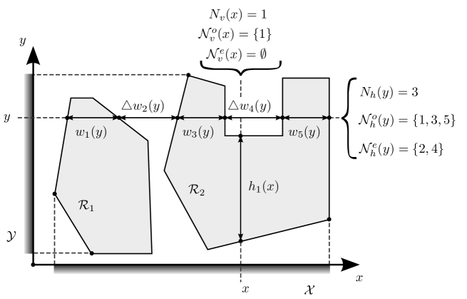
Figure 1: Support region $\mathcal{R}=\mathcal{R}_{1}\bigcup\mathcal{R}_{2}$ of a non-convex uniform map (the notation introduced in Sec. II-A has been adopted). Note that $\mathcal{R}$ (grey region) represents the area where the agent has non-zero probability to lie, so that everything else has to be considered as an “obstruction” (see (1)).

The graphical meaning of these parameters for a specific uniform map is exemplified by Fig. 1.

II-B Observation Modelling

In the following, we assume that the localization system is able to acquire a set of noisy observations, collected in a vector $\mathbf{z}$ and related to the agent position $\mathbf{p}$ according to a specific statistical model. Note that, on the one hand, the results illustrated in Sec. III-A hold for a general statistical model relating $\mathbf{z}$ to $\mathbf{p}$; on the other hand, in Sec. III-B and III-C, it is assumed that

$$f(\mathbf{z}|\mathbf{p})=\mathcal{N}\left(\mathbf{z};\mathbf{p},\boldsymbol{\Sigma}\right)$$ (2)

for mathematical convenience, where $\mathbf{z}\in\mathbb{R}^{2}$ and $\boldsymbol{\Sigma}\triangleq\operatorname{diag}\left\{\sigma_{x}^{2},\sigma_{y}^{2}\right\}$ (i.e., $\mathbf{z}$ is affected by uncorrelated noise). It is important to point out that:

1. The model (2) is purposely abstract and does not explicitly refer to a specific localization technique (e.g., TOA or received signal strength (RSS)) or to particular propagation conditions. Generally speaking, it is suitable to describe the position estimate $\mathbf{z}$ generated by a map-unaware and unbiased localization algorithm; in addition, it leads to useful bounds which unveil the impact of map modelling (instead of that of observation modelling) on estimation performance; readers interested in an in-depth analysis on the impact of observation modelling can refer to [3, 4, 5, 6, 7, 8, 9, 10].

2. In principle, the bounds derived in this manuscript can be extended to the case of correlated noise, accounting for the presence of an off-diagonal term $\sigma_{xy}\neq 0$ in $\boldsymbol{\Sigma}$. However, the presence of noise correlation is neglected in the following derivations since: a) the magnitude of $\sigma_{xy}$ in a real world system depends on several parameters (the type of measurements processed by the system, the multi-lateration or angulation technique employed, the properties of the propagation channel, etc) and cannot be easily assessed; b) our research work evidenced that the presence of noise correlation does not provide significant additional insights on the impact of map-awareness on performance bounds.

III Performance Bounds for Map-Aware Position Estimators

In this Section various bounds about the accuracy of map-aware position estimation are derived and their implications are analysed.

III-A Bayesian Cramer-Rao Bounds

Given an estimator $\hat{\mathbf{p}}(\mathbf{z})$ of $\mathbf{p}$ based on the observation vector $\mathbf{z}$, the BCRB establishes that the Bayesian mean square error (BMSE) matrix

$$\boldsymbol{\Lambda}\left(\hat{\mathbf{p}}(\mathbf{z})\right)\triangleq\mathbb{E}_{\mathbf{z},\mathbf{p}}\left\{\left(\hat{\mathbf{p}}(\mathbf{z})-\mathbf{p}\right)\left(\hat{\mathbf{p}}(\mathbf{z})-\mathbf{p}\right)^{T}\right\}$$

satisfies $\boldsymbol{\Lambda}\left(\hat{\mathbf{p}}(\mathbf{z})\right)\succeq\mathbf{J}^{-1}$ [19, 20], where $\mathbf{J}$ is the Bayesian Fisher information matrix (BFIM) associated to the statistical models employed by $\hat{\mathbf{p}}(\mathbf{z})$. This result entails that, for 2-D localization:

$$\mathbf{E}\triangleq\operatorname{diag}\left\{E_{x},E_{y}\right\}\succeq\mathbf{B}\triangleq\operatorname{diag}\left\{B_{x},B_{y}\right\}$$ (3)

where $E_{x}\triangleq\left[\boldsymbol{\Lambda}\left(\hat{\mathbf{p}}(\mathbf{z})\right)\right]_{1,1}$, $E_{y}\triangleq\left[\boldsymbol{\Lambda}\left(\hat{\mathbf{p}}(\mathbf{z})\right)\right]_{2,2}$, $B_{x}\triangleq\left[\mathbf{J}^{-1}\right]_{1,1}$ and $B_{y}\triangleq\left[\mathbf{J}^{-1}\right]_{2,2}$. It is not difficult to show that the BFIM $\mathbf{J}$ can be put in the form (e.g., see [19, p. 183, eq. (75)])

$$\mathbf{J}=\mathbf{J}_{\mathbf{z|p}}+\mathbf{J}_{\mathbf{p}}$$ (4)

where

$$\mathbf{J}_{\mathbf{z|p}}\triangleq\mathbb{E}_{\mathbf{z},\mathbf{p}}\left\{-\frac{\partial}{\partial\mathbf{p}}\left[\frac{\partial}{\partial\mathbf{p}}\ln f(\mathbf{z}|\mathbf{p})\right]^{T}\right\}$$ (5)

and

$$\mathbf{J}_{\mathbf{p}}\triangleq\mathbb{E}_{\mathbf{p}}\left\{-\frac{\partial}{\partial\mathbf{p}}\left[\frac{\partial}{\partial\mathbf{p}}\ln f(\mathbf{p})\right]^{T}\right\}$$ (6)

represent the contributions originating from the observation vector (i.e., the so called conditional information) and that due to a priori information, respectively. The last decomposition allows us to analyse the two above mentioned sources of information in a separate fashion. Therefore, in the following, we mainly focus on the evaluation of the matrix $\mathbf{J}_{\mathbf{p}}$ (6), since this term unveils the contribution of map information in the estimation of agent position. As already mentioned in Sec. II-A a smoothed uniform map model is adopted in the derivation of $\mathbf{J}_{\mathbf{p}}$ (analytical details are provided in Appendix A) so that its pdf $f(\mathbf{p})$, unlike its (discontinuous) uniform counterpart (1), satisfies the regularity condition[20]

$$\mathbb{E}_{\mathbf{p}}\left\{\frac{\partial}{\partial\mathbf{p}}\ln f(\mathbf{p})\right\}=\mathbf{0}$$ (7)

required for the evaluation of the Bayesian Fisher information. Moreover it is assumed that:

1. the smoothing of $f(\mathbf{p})$ is described by a smoothing function $s(t)$, which is required to be a continuous and differentiable pdf for which the a priori Fisher information (FI) $\mathrm{J}_{s}\triangleq\mathbb{E}_{t}\left\{\left(\frac{\partial\ln s\left(t\right)}{\partial t}\right)^{2}\right\}$ can be evaluated;

2. the smoothing of $f(\mathbf{p})$ along the $x$ axis is independent from that along the $y$ axis.

In Appendix A it is proved that, given the assumptions illustrated above, $\mathbf{J}_{\mathbf{p}}$ (6) can be approximated as

$$\mathbf{J_{p}}\simeq\frac{\mathrm{J}_{s}}{\mathcal{A_{R}}}\operatorname{diag}\left\{\int_{\mathcal{Y}}\sum_{n\in\mathcal{N}_{h}^{o}(y)}\frac{dy}{w_{n}(y)},\int_{\mathcal{X}}\sum_{m\in\mathcal{N}_{v}^{o}(x)}\frac{dx}{h_{m}(x)}\right\}$$ (8)

Note that such an expression is independent from the observation model and depends from the smoothing function through its FI $\mathrm{J}_{s}$ only. Given $\mathbf{J_{p}}$, the computation of the BCRB requires the knowledge of $\mathbf{J}_{\mathbf{z|p}}$ (5) (see (4)); for its evaluation, instead of considering a specific observation model, we just assume that the cross-information about $x$ and $y$ is negligible, so that such a matrix can be put in the form

$$\mathbf{J_{z|p}}=\operatorname{diag}\left\{\mathrm{J}_{\mathbf{z}|x},\mathrm{J}_{\mathbf{z}|y}\right\}$$ (9)

Then, the BCRB associated with the pdf $f(\mathbf{p})$ can be put in the form (see (8), (9) and (4))

$$\mathbf{E}\succeq\mathbf{B}\simeq\operatorname{diag} \left\{\left(\mathrm{J}_{\mathbf{z}|x}+\frac{\mathrm{J}_{s}}{\mathcal{A_{R}}}\int_{\mathcal{Y}}\sum_{n\in\mathcal{N}_{h}^{o}(y)}\frac{dy}{w_{n}(y)}\right)^{-1},\right.$$

$$\quad\left.\left(\mathrm{J}_{\mathbf{z}|y}+\frac{\mathrm{J}_{s}}{\mathcal{A_{R}}}\int_{\mathcal{X}}\sum_{m\in\mathcal{N}_{v}^{o}(x)}\frac{dx}{h_{m}(x)}\right)^{-1}\right\}$$ (10)

It can be shown that the last two expressions are exact, and can be put in a closed form (not involving any integral), if $\mathcal{R}$ is the union of a set of disjoint rectangles (all having parallel sides).

From (8) and (10) it can be inferred that:

1. Map-aware estimators should be expected to be always more accurate than their map-unaware counterparts; in fact $\mathbf{J_{p}}$ (8) is positive definite, so that the trace of the matrix $\mathbf{B}$ (10) (which bounds the accuracy of map-aware estimators) is smaller than the trace of

   $$\left(\mathbf{J_{z|p}}\right)^{-1}=\operatorname{diag}\left\{\mathrm{J}_{\mathbf{z}|x}^{-1},\mathrm{J}_{\mathbf{z}|y}^{-1}\right\}$$

   (see (9)) which represents the Cramer-Rao bound (CRB) in the considered scenario (and bounds the accuracy of map-unaware estimators). Note that this is a well-known result (the contribution of a priori information is positive and lowers the BCRB), but may be concealed by the complex analytical form of (10).

2. The BCRB (10) exhibits a complicated dependence on the map properties and, in particular, a complex non linear dependence on the map area $\mathcal{A_{R}}$; in fact, this parameter can be related to the functions $\left\{h_{m}(x)\right\}$ and $\left\{w_{n}(y)\right\}$ appearing in the right-hand side (RHS) of (10) as

   $$\mathcal{A_{R}}=\int_{\mathcal{Y}}\sum_{n\in\mathcal{N}_{h}^{o}(y)}w_{n}(y)dy=\int_{\mathcal{X}}\sum_{m\in\mathcal{N}_{v}^{o}(x)}h_{m}(x)dx\ .$$

   However, the following asymptotic result suggests that the BCRB is expected to increase (and thus the accuracy of map-aware estimation to worsen) as $\mathcal{A_{R}}$ gets larger: if $\mathcal{A_{R}}\rightarrow\infty$ the BCRB tends to the CRB (since the map support $\mathcal{R}\rightarrow\mathbb{R}^{2}$ and the contribution coming from prior information vanishes) which always takes on a bigger value (see point 1).

3. Only the smallest elements in the set $\left\{w_{n}(y)\right\}$ ($\left\{h_{m}(x)\right\}$) significantly contribute to the sum $\vphantom{A_{A_{A_{A_{A_{A}}}}}}\sum_{n\in\mathcal{N}_{h}^{o}(y)}\frac{1}{w_{n}(y)}$ ($\sum_{m\in\mathcal{N}_{v}^{o}(x)}\frac{1}{h_{m}(x)}$) appearing in (8) and (10) and, consequently, may appreciably influence estimation accuracy; in the limit, if $w_{n}(y)\rightarrow 0$ ($h_{m}(x)\rightarrow 0$) for some $n$ and $y$ ($m$ and $x$), then the information about $x$ ($y$) coordinate becomes infinite because the agent is constrained to lie, for those values of $n$ and $y$ ($m$ and $x$), in a single point of the map support.

4. The matrices $\mathbf{J_{p}}$ (8) and $\mathbf{B}$ (10) can be easily put in a closed form when $\left\{h_{m}(x)\right\}$ and $\left\{w_{n}(y)\right\}$ are step functions (i.e., the map is made by union of rectangles).

Further insights can be obtained taking a specific class of maps into consideration. In particular, here we focus on the case of a map without obstructions, i.e., characterized by a support $\mathcal{R}$ such that $\mathcal{N}_{h}^{e}(y)=\emptyset$ and $\mathcal{N}_{v}^{e}(x)=\emptyset$ $\forall x,y$ (note that convex maps belong to this class); under these assumptions, it is easy to show that $\mathbf{J}_{\mathbf{p}}$ (8) can be simplified as

$$\mathbf{J_{p}}\simeq\frac{\mathrm{J}_{s}}{\mathcal{A_{R}}}\operatorname{diag}\left\{\int_{\mathcal{Y}}\frac{dy}{w_{1}(y)},\int_{\mathcal{X}}\frac{dx}{h_{1}(x)}\right\}$$ (11)

From the RHS of the last expression it can be easily inferred that:

$$\mathbf{E}\succeq\mathbf{Z}=\operatorname{diag} \left\{\frac{\sigma_{x}^{3}}{2\mathcal{\mathcal{A_{R}}}}\int_{\mathcal{Y}}\left[\sum_{n\in\mathcal{N}_{h}^{o}(y)}\zeta\left(\frac{w_{n}(y)}{\sigma_{x}}\right)+\sum_{n\in\mathcal{N}_{h}^{e}(y)}\zeta_{ov}\left(\frac{\triangle w_{n}(y)}{\sigma_{x}},\frac{w_{n-1}(y)}{\sigma_{x}},\frac{w_{n+1}(y)}{\sigma_{x}}\right)\right]dy,\right.$$

$$\left.\frac{\sigma_{y}^{3}}{2\mathcal{A_{R}}}\int_{\mathcal{X}}\left[\sum_{m\in\mathcal{N}_{v}^{o}(x)}\zeta\left(\frac{h_{m}(x)}{\sigma_{y}}\right)+\sum_{m\in\mathcal{N}_{v}^{e}(x)}\zeta_{ov}\left(\frac{\triangle h_{m}(x)}{\sigma_{y}},\frac{h_{m-1}(x)}{\sigma_{y}},\frac{h_{m+1}(x)}{\sigma_{y}}\right)\right]dx\right\}$$ (14)

1. Even in this case the dependence of $\mathbf{J_{p}}$ from $\mathcal{A_{R}}$ is complicated. However, analysing (11), it is easy to note that if $\mathcal{R}\rightarrow\mathbb{R}^{2}$ (so that $\mathcal{A_{R}}\rightarrow\infty$) the elements of $\mathbf{J_{p}}$ tend to zero, so that the impact of prior information vanishes, as already mentioned above.

2. The amount of information concerning the agent position along the $x$ ($y$) axis direction is proportional to $\int_{\mathcal{Y}}\tilde{w}(y)dy$ ($\int_{\mathcal{X}}\tilde{h}(x)dx$), where $\tilde{w}(y)\triangleq 1/w_{1}(y)$ ($\tilde{h}(x)\triangleq 1/h_{1}(x)$); the last integral can be interpreted as the area of a “virtual map” characterized by the same projection $\mathcal{Y}$ ($\mathcal{X}$) as the real map, but whose width (height) at each point $y\mathcal{\in Y}$ ($x\mathcal{\in X}$) is the reciprocal of the width (height) of the real map.

3. When prior information dominates over conditional information, the map support $\mathcal{R}$ minimizing the trace of the BCRB under the constraint of a constant area $\mathcal{A_{R}}$ has a square shape. In fact, if $\mathcal{R}$ is a rectangle whose sides have lengths $L_{x}$ and $L_{y}$, it is easy to show that $\mathbf{J_{p}}=\frac{\mathrm{J}_{s}}{\mathcal{A_{R}}}\operatorname{diag}\left\{\frac{L_{y}}{L_{x}},\frac{L_{x}}{L_{y}}\right\}=\mathrm{J}_{s}\operatorname{diag}\left\{\frac{1}{L_{x}^{2}},\frac{1}{L_{y}^{2}}\right\}$; then, if we set $L_{x}=\gamma L$, $L_{y}=\frac{L}{\gamma}$, where $\gamma$ and $L$ denote two real positive parameters, the trace of the inverse of (11) can be put in the form $\frac{L^{2}}{\mathrm{J}_{s}}\left(\gamma^{2}+1/\gamma^{2}\right)$ and is minimized for $\gamma=1$ (i.e., for $L_{x}=L_{y}$).

4. In (11) the only contribution coming from the smoothing function $s(t)$ is represented by the factor $\mathrm{J}_{s}$.

Further comments about the BCRB (10) will be provided in Section IV, where this bound is computed for some specific maps.

Finally, it is important to point out that: a) in localization problems BCRB’s often provide useful insights [10, 12, 9], but these bounds are usually loose for low SNR conditions [22, 23], i.e., when a priori information (the map in this context) plays a critical role due to the poor quality of observations; b) the BCRB analysis requires the adoption of the smoothed uniform pdf model for prior information (see Section II-A).

These considerations motivate the search for other bounds and, in particular, for the EZZB, which is usually tighter than the BCRB at low SNRs [24, 23, 25, 26, 27] and does not require (7) to hold (so that the uniform model (1) can be employed as it is); this is further discussed in the following section.

III-B Zik-Zakai Bounds

Similarly to (3), the EZZB for 2D localization can be expressed as

$$\mathbf{\mathbf{E}}\triangleq\operatorname{diag}\left\{E_{x},E_{y}\right\}\succeq\mathbf{Z}\triangleq\operatorname{diag}\left\{Z_{x},Z_{y}\right\}$$ (12)

where (see Appendix B)

$$Z_{\nu}\triangleq\frac{1}{2}\iint_{\mathcal{P}_{\nu}}\left[f\left(\boldsymbol{\rho}\right)+f\left(\boldsymbol{\rho}+h\mathbf{e}_{\nu}\right)\right]P_{\text{\tiny{min}}}^{\mathbf{z}}\left(\boldsymbol{\rho},\boldsymbol{\rho}+h\mathbf{e}_{\nu}\right)h\,d\boldsymbol{\rho}dh$$ (13)

$\nu\in\{x,y\}$, $\mathbf{e}_{x}\triangleq[1,0]^{T}$, $\mathbf{e}_{y}\triangleq[0,1]^{T}$, $P_{\text{\tiny{min}}}^{\mathbf{z}}(\boldsymbol{\rho},\boldsymbol{\rho}+h\mathbf{e}_{\nu})$ represents the error probability referring to the likelihood ratio test in a binary detection problem involving the hypotheses

$$H_{0}:\>\mathbf{p}=\boldsymbol{\rho}$$

$$H_{1}:\>\mathbf{p}=\boldsymbol{\rho}+h\mathbf{e}_{\nu}$$

and the observation $\mathbf{z}$; finally, the integration domain is

$$\mathcal{P}_{\nu}\triangleq\left\{\left(h,\boldsymbol{\rho}\right):h\geq 0\wedge f\left(\boldsymbol{\rho}\right)>0\wedge f\left(\boldsymbol{\rho}+h\mathbf{e}_{\nu}\right)>0\right\}\subset\mathbb{R}^{3}$$

The EZZB (12)-(13) deserves the following comments:

1. its formulation is obtained from the standard formulation (see [25, Eq. (32)]) removing the so-called valley-filling function and the maximization operator, as shown in Appendix B; these modifications simplify the derivation of the bound at the price of a small reduction in its tightness;

2. it exhibits a complicated dependence on the observation model, which comes into play in the evaluation of the probability $P_{\text{\tiny{min}}}^{\mathbf{z}}\left(\boldsymbol{\rho},\boldsymbol{\rho}+h\mathbf{e}_{\nu}\right)$;

3. it cannot be put in a form similar to (4), so that, generally speaking, the contribution coming from conditional information (i.e., observations) cannot be easily separated from that associated with a priori information (map awareness in this case).

As shown in Appendix B, for a uniform map and the observation model (2) the EZZB (13) can be put in the form (14) shown at the top of this page where

$$\zeta(\rho)\triangleq\int_{0}^{\rho}(\rho-u)u\operatorname{erfc}\left(\frac{u}{2\sqrt{2}}\right)du$$ (15)

$$\zeta_{ov}\left(\rho_{\triangle},\rho_{1},\rho_{2}\right)\triangleq\\ \int_{\rho_{\triangle}}^{\rho_{\triangle}+\rho_{2}}(u-\rho_{\triangle})u\operatorname{erfc}\left(\frac{u}{2\sqrt{2}}\right)du+\\ \int_{\rho_{\triangle}+\rho_{2}}^{\rho_{\triangle}+\rho_{1}}\rho_{2}u\operatorname{erfc}\left(\frac{u}{2\sqrt{2}}\right)du+\\ \int_{\rho_{\triangle}+\rho_{1}}^{\rho_{\triangle}+\rho_{1}+\rho_{2}}(\rho_{\triangle}+\rho_{1}+\rho_{2}-u)u\operatorname{erfc}\left(\frac{u}{2\sqrt{2}}\right)du$$ (16)

An accurate analysis of the EZZB (14) and a comparison with the BCRB (10) lead to the following conclusions:

1. The EZZB (14) exhibits a similar dependence as the BCRB (10) in terms of the quantities $\{w_{n}(y)\}$, $\{h_{m}(y)\}$. In fact, if $\{w_{n}(y)\}$ and/or $\{h_{m}(x)\}$ increases, the trace of matrix $\mathbf{Z}$ in (14) gets larger, since $\zeta$ (15) is a monotonically increasing function.

2. In the same environment the EZZB (14) takes on larger values than the BCRB (10) and results to be a bound tighter to the performance of optimal estimators. This is due to the fact that the terms $\zeta$ appearing in the RHS of (14) give the EZZB approximately the same behaviour of the BCRB; however, the EZZB also contains terms based on $\zeta_{ov}$ (16), which is a positive valued function.

3. The EZZB (14), unlike the BCRB, is influenced by the shape of map obstructions (through the $\zeta_{ov}$ function and the $\left\{\triangle w_{n}(y)\right\}$, $\left\{\triangle h_{m}(y)\right\}$ parameters).

4. The two terms of (14) depending on the function $\zeta_{ov}$ (16) are influenced by the spatial extensions $\left\{\triangle w_{n}(y)\right\}$ and $\left\{\triangle h_{m}(y)\right\}$ of the obstructions separating consecutive map segments (which are characterized by the lengths $\{w_{n-1}(y),w_{n+1}(y)\}$ and $\{h_{m-1}(y),h_{m+1}(y)\}$, respectively); in particular, the impact of obstructions is significant when $\triangle w_{n}(y)$ ($\triangle h_{m}(y)$) is greater than one of $\{w_{n-1}(y),w_{n+1}(y)\}$ ($\{h_{m-1}(y),h_{m+1}(y)\}$).

5. The integrals in the RHS of (14) can be easily put in a closed form when $\left\{h_{m}(x)\right\}$ and $\left\{w_{n}(y)\right\}$ are step functions (i.e., the map is made by union of rectangles).

Similarly to the BCRB, further insights can be obtained considering the class of maps without obstructions. In this case the EZZB (14) simplifies as

$$\mathbf{E} \succeq\mathbf{W}=\operatorname{diag}\left\{\sup_{h_{x}\in\mathbb{R}}\frac{\left[h_{x}\exp\left(-\frac{h_{x}^{2}}{8\sigma_{x}^{2}}\right)\lambda_{x}\left(h_{x},\mathcal{R}\right)\right]^{2}}{2\mathcal{\mathcal{A_{R}}}\left[\lambda_{x}\left(h_{x},\mathcal{R}\right)-\exp\left(-\frac{h_{x}^{2}}{2\sigma_{x}^{2}}\right)\gamma_{x}\left(h_{x},\mathcal{R}\right)\right]},\sup_{h_{y}\in\mathbb{R}}\frac{\left[h_{y}\exp\left(-\frac{h_{y}^{2}}{8\sigma_{y}^{2}}\right)\lambda_{y}\left(h_{y},\mathcal{R}\right)\right]^{2}}{2\mathcal{\mathcal{A_{R}}}\left[\lambda_{y}\left(h_{y},\mathcal{R}\right)-\exp\left(-\frac{h_{y}^{2}}{2\sigma_{y}^{2}}\right)\gamma_{y}\left(h_{y},\mathcal{R}\right)\right]}\right\}$$ (22)

$$\mathbf{E}\succeq\mathbf{Z}=\frac{1}{2\mathcal{\mathcal{A_{R}}}}\operatorname{diag} \left\{\sigma_{x}^{3}\int_{\mathcal{Y}}\zeta\left(\frac{w_{1}(y)}{\sigma_{x}}\right)dy,\right.$$

$$\>\>\>\left.\sigma_{y}^{3}\int_{\mathcal{X}}\zeta\left(\frac{h_{1}(x)}{\sigma_{y}}\right)dx\right\}$$ (17)

It is also worth mentioning that, if the map support $\mathcal{R}$ can be expressed as the union of a set of disjoint rectangles (all having parallel sides), the EZZB (17) can be simplified further, obtaining a closed-form bound.

The result (17) deserves the following comments:

1. The structure of its RHS is similar to that of the equivalent BFIM (11). Despite the differences between the integrand functions, our numerical results show that in this case both the EZZB and the BCRB are tight and that the EZZB does not provide additional hints on localization accuracy with respect to the BCRB (see Section IV).

2. The EZZB predicts the correct variance of map-aware estimation when the SNR is very low whereas a specific assumption about the value of $\mathrm{J}_{s}$ is required to obtain the same result in the BCRB case. For instance, let us consider a uniform map whose support $\mathcal{R}$ is a rectangle whose sides have lengths $L_{x}$ and $L_{y}$; with model (2) and for $\sigma_{x}^{2}\rightarrow\infty$ and $\sigma_{y}^{2}\rightarrow\infty$ (i.e., for a SNR approaching zero), the BMSE of the minimum mean square error (MMSE) estimator tends to $\operatorname{diag}\left\{L_{x}^{2}/12,L_{y}^{2}/12\right\}$. The EZZB provides this exact result since the RHS of (17) can be put in the closed form

   $$\mathbf{Z}=\operatorname{diag}\left\{\frac{\sigma_{x}^{3}}{2L_{x}}\zeta\left(\frac{L_{x}}{\sigma_{x}}\right),\frac{\sigma_{y}^{3}}{2L_{y}}\zeta\left(\frac{L_{y}}{\sigma_{y}}\right)\right\}$$ (18)

   and $\zeta(\rho)/(2\rho)\rightarrow\rho^{2}/12$ for a SNR $\rho$ approaching zero. This result can be compared with its BCRB counterpart; in this case, from (11) it can be inferred that $\mathbf{B}\mathbf{\rightarrow}\operatorname{diag}\left\{L_{x}^{2}/J_{s},L_{y}^{2}/J_{s}\right\}$, so that $J_{s}=12$ should be selected to match the correct variance.

3. The EZZB (17) confirms that map-aware estimators should be expected to be more accurate than their map-unaware counterparts, at least for maps without obstructions: for instance, if a rectangular map of sides $L_{x}$, $L_{y}$ is considered, then (18) is easily proved to be always smaller than $\operatorname{diag}\left\{\sigma_{x}^{2},\sigma_{y}^{2}\right\}$ (because $0\leq\zeta(\rho)/(2\rho)<1$) which is the trivial EZZB for the observation model (2) when the map is unavailable (i.e., when no prior information is available). This derives from the fact that a priori information lowers the EZZB (similarly to what occurs in the case of the CRB and the BCRB); this is a well-known result, but may not be evident in (17).

4. Similarly to the BCRB, the dependence on the map area is complicated; however, it should be expected that the elements of $\mathbf{Z}$ get larger when $\mathcal{\mathcal{A_{R}}}$ increases as suggested by the following asymptotic result: when $\mathcal{A_{R}}\rightarrow\infty$ the contribution coming from a priori information vanishes and the EZZB (18) tends to $\operatorname{diag}\left\{\sigma_{x}^{2},\sigma_{y}^{2}\right\}$, i.e., to the map-unaware EZZB, which is larger (see point 3).

As already mentioned above, the EZZB allows us to understand the role played by some map features, which do not have any impact on the BCRB. However, our numerical results evidence that, for complex maps and, in particular, at very low SNRs, this bound turns out to be somewhat far from the performance offered by a MMSE estimator. This has motivated the derivation of the WWB [28], which can be tighter than the EZZB at very low-SNRs.

III-C Wess-Weinstein Bounds

Similarly to the BCRB and the EZZB (see (3) and (12), respectively), the WWB, for 2-D localization, can be expressed as

$$\mathbf{E}\succeq\mathbf{W}\triangleq\operatorname{diag}\left\{W_{x},W_{y}\right\}$$ (19)

where [29]

$$W_{\nu}\triangleq\sup_{h_{\nu}\in\mathbb{R}}\frac{\left(h_{\nu}\mathbb{E}_{\mathbf{z},\mathbf{p}}\left\{L^{\frac{1}{2}}\left(\mathbf{z};\mathbf{p}^{+},\mathbf{p}\right)\right\}\right)^{2}}{\mathbb{E}_{\mathbf{z},\mathbf{p}}\left\{\left[L^{\frac{1}{2}}\left(\mathbf{z};\mathbf{p}^{+},\mathbf{p}\right)-L^{\frac{1}{2}}\left(\mathbf{z};\mathbf{p}^{-},\mathbf{p}\right)\right]^{2}\right\}}$$ (20)

and

$$\mathbf{p}^{+}\triangleq\mathbf{p}+h_{\nu}\mathbf{e}_{\nu}$$

$$\mathbf{p}^{-}\triangleq\mathbf{p}-h_{\nu}\mathbf{e}_{\nu}$$

are functions of the $h_{\nu}$ parameter; moreover

$$L\left(\mathbf{z};\mathbf{p}_{1},\mathbf{p}_{2}\right)\triangleq\frac{f(\mathbf{z},\mathbf{p}_{1})}{f(\mathbf{z},\mathbf{p}_{2})}=\frac{f(\mathbf{z}|\mathbf{p}_{1})f(\mathbf{p}_{1})}{f(\mathbf{z}|\mathbf{p}_{2})f(\mathbf{p}_{2})}$$ (21)

is a likelihood ratio and $\nu\in\{x,y\}$. Note that (20) can be obtained from [29, Eqs. (7)-(8)] setting $N=2$, $s_{1}=s_{2}=\frac{1}{2}$ for the WWB optimization parameters and $\mathbf{H}=\operatorname{diag}\left\{h_{x},h_{y}\right\}$, since we are interested in a bound on the variance (not on the co-variance) of the estimates of $\mathbf{p}$.

As shown in Appendix C, for a uniform map and the observation model (2) the WWB (20) can be put in the form (22) shown at the top of the next page, where $h_{x}$, $h_{y}$ denote the parameters to be optimized to make the bound tighter,

$$\lambda_{x}\left(h_{x},\mathcal{R}\right)\triangleq\int\mathbb{I}_{\mathcal{R}}(\mathbf{p})\mathbb{I}_{\mathcal{R}}(\mathbf{p}+h_{x}\mathbf{e}_{x})d\mathbf{p}\\ =\int_{\mathcal{Y}}\sum_{n\in\mathcal{N}_{h}^{o}(y)}\omega\left(w_{n}(y),h_{x}\right)dy+\\ \int_{\mathcal{Y}}\sum_{n\in\mathcal{N}_{h}^{e}(y)}\omega_{ov}\left(\triangle w_{n}(y),w_{n-1}(y),w_{n+1}(y),h_{x}\right)dy$$ (23)

and

$$\gamma_{x}\left(h_{x},\mathcal{R}\right) \triangleq\int\mathbb{I}_{\mathcal{R}}(\mathbf{p})\mathbb{I}_{\mathcal{R}}(\mathbf{p}+h_{x}\mathbf{e}_{x})\mathbb{I}_{\mathcal{R}}(\mathbf{p}-h_{x}\mathbf{e}_{x})d\mathbf{p}$$

$$=2\int_{\mathcal{Y}}\sum_{n\in\mathcal{N}_{h}^{o}(y)}\omega\left(\frac{1}{2}w_{n}(y),h_{x}\right)dy$$ (24)

are functions of the parameters $h_{x}$, $h_{y}$ and of the geometrical features of the map support $\mathcal{R}$ (dual expressions hold for $\lambda_{y}\left(h_{y},\mathcal{R}\right)$ and $\gamma_{y}\left(h_{y},\mathcal{R}\right)$); finally

$$\omega\left(w,h_{x}\right)\triangleq(w-h_{x})\mathbb{I}_{[0;w]}(h_{x})$$ (25)

$$\omega_{ov}\left(\triangle w,w_{1},w_{2},h\right)\triangleq\\ \begin{cases}h-\triangle w&h\in[\triangle w;\triangle w+w_{2}]\\ w_{2}&h\in[\triangle w+w_{2};\triangle w+w_{1}]\\ w_{tot}-h&h\in[\triangle w+w_{1};w_{tot}]\end{cases}$$ (26)

$$w_{tot}\triangleq\triangle w+w_{1}+w_{2}\ .$$

Note that the structure of $\lambda_{x}\left(h_{x},\mathcal{R}\right)$ (23) is similar to that of some terms contained in the RHS of the EZZB (14); however, in the WWB the noise variances appear in some exponential functions (22) only.

Unfortunately, it is hard to infer from (22) any conclusion about the dependence of the WWB on the features of a given map; this is mainly due to the presence of the $\sup\left(\cdot\right)$ operators and to the discontinuous behaviour of the functions $\omega\left(\cdot\right)$ and $\omega_{ov}\left(\cdot\right)$. Despite this, the WWB may play an important role, since, as shown in Section IV for specific maps, it is tighter than the BCRB and the EZZB at low-SNRs.

In the following Section the general bounds provided above are evaluated for specific maps, so that some additional insights about the ultimate accuracy achieved by map-aware estimators can be obtained.

IV Numerical Results

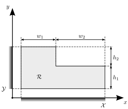
Figure 2: Support region $\mathcal{R}$ of a “L-shaped” map (map #2).

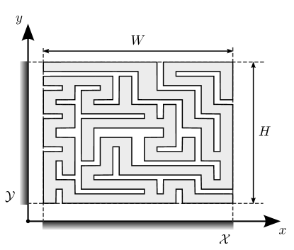
Figure 3: Support region $\mathcal{R}$ of a map modelling the floor of a big building (map #3).

The bounds illustrated in the previous Section have been evaluated for the following 3 specific maps:

1. map #1: a unidimensional map whose support $\mathcal{R}$ consists of $N_{r}=2$ disjoint segments (denoted $\mathcal{R}_{1}$ and $\mathcal{R}_{2}$ in the following) having the same length $w$ and separated by $\triangle x$ meters;

2. map #2: the “L-shaped” 2-D map shown in Fig. 2 and fully described by the set $\left\{w_{1},w_{2},\right.$ $\left.h_{1},h_{2}\right\}$ of geometrical parameters;

3. map #3: the 2-D map shown in Fig. 3; note that such a map models the floor of a large building and is quite complex, so that its geometrical parameters are not given and analytical bounds are not evaluated for it; instead, some numerical results generated by means of computer simulations will be illustrated.

It is important to point out that maps #2 and #3 are examples of 2-D rectangular uniform maps, i.e., each of them is characterised by a support $\mathcal{R}$ that can be represented as the union of non-overlapping rectangles, all having parallel sides; such non-overlapping rectangles form the so called rectangular covering of the map support $\mathcal{R}$ [30, 31, 32]. Note that any map characterised by a support of arbitrary shape can be always approximated, up to an arbitrary precision, by a rectangular map if a proper covering, containing a sufficiently large number of rectangles, is selected. For this reason, maps #2 and #3 are relevant and practical examples. Map #1 can be also deemed relevant from a practical point of view since it can be thought of as a transversal slice of a 2-D map (consisting, for instance, of two road lanes or two rooms facing each other); in addition, such a simple scenario allows to acquire more insights than maps #2 and #3, as shown later.

In all cases the observation model (2) has been adopted (with $\boldsymbol{\Sigma}=\sigma^{2}$ and $\boldsymbol{\Sigma}=\sigma^{2}\mathbf{I}_{2}$ in the 1-D and 2-D scenarios, respectively) and the tightness of the bounds has been assessed comparing them with the root mean square error (RMSE) performance of optimal estimators evaluated by means of extensive computer simulations. In addition, in accordance with the theoretical arguments of Paragraph III-B (see the comments to (17)), $J_{s}=12$ has been selected in the evaluation of all the BCRB results illustrated in this Section. Finally, in our simulations $N_{runs}=10^{4}$ realizations of the random parameter $\mathbf{p}$ have been generated according to a uniform distribution over the map support $\mathcal{R}$; then Gaussian noise samples (characterized by $\sigma=3\,\text{m}$ if not explicitly stated) have been added to generate the noisy observations, according to (2).

IV-A Map #1

Bounds - The BCRB, the EZZB and WWB for map #1 are (see (10), (14), and (22), respectively)

$$E_{x}\geq B_{x}=\sigma^{2}\frac{\rho^{2}}{\rho^{2}+\mathrm{J}_{s}}$$ (27)

$$E_{x}\geq Z_{x}=\frac{\sigma^{2}}{4\rho}\left[2\zeta(\rho)+\zeta_{ov}(\rho_{\triangle},\rho,\rho)\right]$$ (28)

and $E_{x}\geq W_{x}$, respectively, where

$$W_{x} =\sup_{h\in\mathbb{R}}\frac{h^{2}\exp\left(-\frac{h^{2}}{4\sigma^{2}}\right)\lambda^{2}\left(h,w,\triangle x\right)}{4w\left[\lambda\left(h,w,\triangle x\right)-\exp\left(-\frac{h^{2}}{2\sigma^{2}}\right)\gamma\left(h,w,\triangle x\right)\right]}$$ (29)

$\rho\triangleq w/\sigma$ is the SNR, $\rho_{\triangle}\triangleq\triangle x/\sigma$,

$$\lambda\left(h,w,\triangle x\right)\triangleq 2\omega\left(w,h\right)+\omega_{ov}\left(\triangle x,w,w,h\right)$$

and $\gamma\left(h,w,\triangle x\right)\triangleq 2\omega\left(\frac{1}{2}w,h\right)$. It is important to point out that that no approximations have been adopted in the derivations of the BCRB, the EZZB and the WWB for the considered 1-D scenario, so that (27)-(29) represent exact bounds (of course, a smoothed uniform map has been assumed for the BCRB only).
Estimators - Map-aware localization can be accomplished exploiting the MMSE estimator

$$\hat{x}_{\text{\tiny{MMSE}}}(z)=(1/c(z))\sum_{n=1}^{N_{r}}\int_{\mathcal{R}_{n}}x\,\mathcal{N}\left(z;x,\sigma^{2}\right)dx$$ (30)

where $c(z)\triangleq\sum_{n=1}^{N_{r}}\int_{\mathcal{R}_{n}}\mathcal{N}\left(z;x,\sigma^{2}\right)dx$ is a normalization factor, or the maximum-a-posteriori (MAP) estimator

$$\hat{x}_{\text{\tiny{MAP}}}(z)=\arg\max_{\tilde{x}\in\mathcal{R}}\mathcal{N}\left(z;\tilde{x},\sigma^{2}\right)$$ (31)

On the contrary, if the map is unknown, the (map-unaware) maximum likelihood (ML) estimator $\hat{x}_{\text{\tiny{ML}}}(z)=z$ can be used (obviously, the resulting estimate has the same variance $\sigma^{2}$ as the observation noise). Note that the RMSE performance of these estimators is influenced by the geometrical parameters $w$ and $\triangle x$ and by the noise standard deviation $\sigma$.
Numerical results - Figs. 4 and 5 compare the square roots of the BCRB, EZZB and WWB bounds $\sqrt{B_{x}}$, $\sqrt{Z_{x}}$, $\sqrt{W_{x}}$ and the RMSE of $\hat{x}_{\text{\tiny{MMSE}}}(z)$, $\hat{x}_{\text{\tiny{MAP}}}(z)$ and $\hat{x}_{\text{\tiny{ML}}}(z)$ versus $\rho$ (with $w$ and $\triangle x$ fixed) and $\triangle x$ (with $w$ and $\sigma$ fixed), respectively.

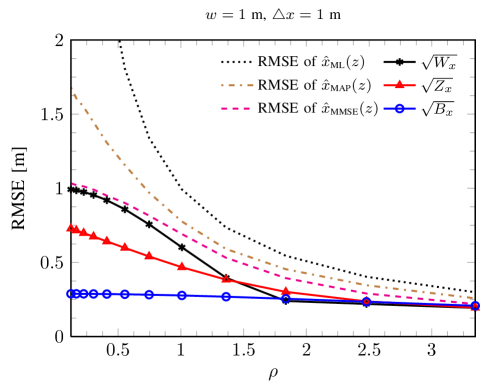
Figure 4: RMSE versus the SNR $\rho$ for the MMSE (30), MAP (31) and ML estimators. Map #1, $w=1\,\text{m}$ and $\triangle x=1\,\text{m}$ are assumed. The BCRB (27), EZZB (28) and WWB (29) are shown for comparison.

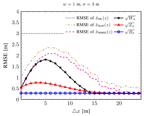
Figure 5: RMSE versus $\triangle x$ for the MMSE (30), MAP (31) and ML estimators. Map #1, $w=1\,\text{m}$ and $\sigma=3\,\text{m}$ are assumed. The BCRB (27), EZZB (28) and WWB (29) are shown for comparison.

These results evidence that:

1. The BCRB is tight at high SNRs only; in such conditions all the bounds and the RMSE of both map-aware and map-unaware estimators tend to $\sigma$ (see Fig. 4): conditional knowledge dominates.

2. Unlike the BCRB, the EZZB and, in particular, the WWB exhibit a dependence on $\triangle x$ and are much tighter (see Fig. 5) to the performance of optimal estimators and, for this reason, represent more useful tools for predicting system accuracy.

3. The role played by map knowledge in estimation accuracy becomes significant as $\rho$ decreases, i.e., as the quality of the observations gets worse; indeed map knowledge prevents the bounds and the RMSE of the map-aware estimators from diverging (note that in Fig. 4 the map-unaware RMSE diverges for $\rho\rightarrow 0$).

4. The performance gap among the MMSE, the MAP and especially the ML estimators is significant for low SNRs (see Fig. 4).

5. If the gap $\triangle x$ is small (i.e., if the segments $\mathcal{R}_{1}$ and $\mathcal{R}_{2}$ are close), the RMSE of the considered estimators is low. On the contrary, if $\triangle x$ increases, the RMSE gets larger, reaches a maximum and then decreases, tending to $w/\sqrt{12}$ (see Fig. 5). This behaviour can be explained as follows: if the noise level is large with respect to $\triangle x$, the estimate of the agent position may belong to the wrong segment, thus resulting in a large error. However, a further increase of $\triangle x$ entails a reduction of the RMSE, since, for a large spacing between $\mathcal{R}_{1}$ and $\mathcal{R}_{2}$, it is unlikely that the wrong segment is selected in map-aware estimation.

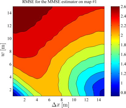
Figure 6: RMSE versus $\triangle x$ and $w$ for the MMSE estimator (30). Map #1 and $\sigma=3\,\text{m}$ are assumed. The data has been smoothed to remove simulation noise and improve readability.

Further insights are provided by Fig. 6, which shows the RMSE versus $w$ and $\triangle x$ for the MMSE estimator (note that the MMSE data shown in Fig. 5 can be extracted from Fig. 6 setting $w=1\,\text{m}$). In fact, the numerical results shown in this figure evidence that:

1. For $w>3\sigma$ the RMSE decreases only mildly as $\triangle x$ gets larger and the main geometric feature of the map affecting estimation accuracy is the area of $\mathcal{R}$; in this case a map-aware estimator still provides an advantage over map-unaware counterparts (the maximum RMSE for the first estimator is $2.6\,\text{m}$, as shown in Fig. 6, and is smaller than $\sigma=3\,\text{m}$, which represents the RMSE for the ML estimator, as shown in Fig. 5).

2. For $w<3\sigma$ the RMSE reaches its maximum for $\triangle x\simeq 3\sigma-w$; for this reason, any combination of the geometric parameters and noise level satisfying such equality should be avoided.

Based on the numerical results shown in Fig. 6, we can draw some observations about an indoor localization system operating in two adjacent rooms, each having width $w_{room}$ and separated by a wall having thickness $\triangle x_{wall}=0.2\,\text{m}$, and processing noisy observations characterized by $\sigma=3\,\text{m}$ (realistic value for RSS systems, see [34, 35, 36]). From Fig. 6 we can infer that, even if $w_{room}<3\sigma=9\,\text{m}$, since $\triangle x_{wall}$ is appreciably smaller than $3\sigma-w$, the advantage in terms of RMSE provided by a map modelling wall obstructions is small with respect to that offered by a map modelling the environment as a single connected room having width $2w_{room}+\triangle x_{wall}$. In fact, in Fig. 6, if the presence of the wall is accounted for, the map-aware estimator performance is associated with the point $(\triangle x_{wall},w_{room})$, whereas, if it is not, with the point $(0,w_{room}+\frac{1}{2}\triangle x_{wall})$. Unless the room size $w_{room}$ is very small (i.e., $w_{room}\simeq\triangle x_{wall}$) the two “operating points” will be very close (due to the small value of $\triangle x_{wall}$) and the resulting RMSE values will be similar so that, in this case, a map modelling wall obstructions is not very useful. Note also that, if the quality of observations improves substantially (i.e., $\sigma\rightarrow 0$), map information plays a less significant role than the conditional information provided by such observations, so that a detailed a priori map modelling walls is not useful in this case, too. On the contrary, maps may play an important role in localization in outdoor environments, where the region characterized by $w<3\sigma$ and $\triangle x\ll 3\sigma-w$ in the $(\triangle x,w)$ plane is easier to reach, since noisy observations and large obstructions should be expected; for this reason, in this case the presence of the obstructions in map modelling should not be neglected.

IV-B Map #2

$$\mathbf{E} \succeq\mathbf{W}=\operatorname{diag}\left\{\sup_{h_{x}\in\mathbb{R}}\frac{h_{x}^{2}\exp\left(-\frac{h_{x}^{2}}{4\sigma^{2}}\right)\lambda_{x}^{2}\left(h_{x},\mathcal{R}\right)}{2\mathcal{A_{R}}\left[\lambda_{x}\left(h_{x},\mathcal{R}\right)-\exp\left(-\frac{h_{x}^{2}}{2\sigma^{2}}\right)\gamma_{x}\left(h_{x},\mathcal{R}\right)\right]},\right.\left.\sup_{h_{y}\in\mathbb{R}}\frac{h_{y}^{2}\exp\left(-\frac{h_{y}^{2}}{4\sigma^{2}}\right)\lambda_{y}^{2}\left(h_{y},\mathcal{R}\right)}{2\mathcal{A_{R}}\left[\lambda_{y}\left(h_{y},\mathcal{R}\right)-\exp\left(-\frac{h_{y}^{2}}{2\sigma^{2}}\right)\gamma_{y}\left(h_{y},\mathcal{R}\right)\right]}\right\}$$ (34)

Bounds - Let us now focus on map #2. The BCRB and the EZZB in this case are (see (10) and (14), respectively)

$$\mathbf{E}\succeq\mathbf{B}=\operatorname{diag} \left\{\sigma^{2}\frac{\rho_{\mathcal{A}}^{2}}{\rho_{\mathcal{A}}^{2}+\mathrm{J}_{s}\left(\frac{h_{2}}{w_{1}}+\frac{h_{1}}{w_{1}+w_{2}}\right)},\right.$$

$$\quad\left.\sigma^{2}\frac{\rho_{\mathcal{A}}^{2}}{\rho_{\mathcal{A}}^{2}+\mathrm{J}_{s}\left(\frac{w_{2}}{h_{1}}+\frac{w_{1}}{h_{1}+h_{2}}\right)}\right\}$$ (32)

$$\mathbf{E}\succeq\mathbf{Z}=\operatorname{diag} \left\{\frac{\sigma^{2}}{2\rho_{\mathcal{A}}}\left[h_{1}\zeta\left(\frac{w_{1}+w_{2}}{\sigma}\right)+h_{2}\zeta\left(\frac{w_{1}}{\sigma}\right)\right],\right.$$

$$\quad\left.\frac{\sigma^{2}}{2\rho_{\mathcal{A}}}\left[w_{1}\zeta\left(\frac{h_{1}+h_{2}}{\sigma}\right)+w_{2}\zeta\left(\frac{h_{1}}{\sigma}\right)\right]\right\}$$ (33)

respectively, where $\rho_{\mathcal{A}}\triangleq\mathcal{A_{R}}/\sigma$. The WWB derived from (22) is shown in (34) at the top of the next page; in (34) the $\lambda_{x}\left(h_{x},\mathcal{R}\right)$ and $\gamma_{x}\left(h_{x},\mathcal{R}\right)$ functions have the expressions

$$\lambda_{x}\left(h_{x},\mathcal{R}\right)=h_{1}\omega(w_{1}+w_{2},h_{x})+h_{2}\omega(w_{1},h_{x})$$

$$\gamma_{x}\left(h_{x},\mathcal{R}\right)=2h_{1}\omega\left(\frac{w_{1}+w_{2}}{2},h_{x}\right)+2h_{2}\omega\left(\frac{w_{1}}{2},h_{x}\right)$$

respectively (dual expressions hold for $\lambda_{y}\left(h_{y},\mathcal{R}\right)$ and $\gamma_{y}\left(h_{y},\mathcal{R}\right)$). Note that $h_{1}$ and $h_{2}$ ($w_{1}$ and $w_{2}$) play a symmetric role in (32), (33) and (34); this suggests that a change in the geometrical features improving $B_{x}$ will reduce $B_{y}$ and vice versa, when the overall area $\mathcal{A_{R}}$ of the map is kept constant.
Estimators - Map-aware localization can be accomplished exploiting the MMSE estimator

$$\hat{\mathbf{p}}_{\text{\tiny{MMSE}}}(\mathbf{z})\triangleq\left[\begin{array}[]{c}\hat{x}_{\text{\tiny{MMSE}}}\\ \hat{y}_{\text{\tiny{MMSE}}}\end{array}\right]=(1/c(\mathbf{z}))\iint_{\mathcal{R}}\mathbf{p}\,\mathcal{N}\left(\mathbf{z};\mathbf{p},\boldsymbol{\Sigma}\right)d\mathbf{p}$$ (35)

where $c(\mathbf{z})\triangleq\iint_{\mathcal{R}}\mathcal{N}\left(\mathbf{z};\mathbf{p},\boldsymbol{\Sigma}\right)d\mathbf{p}$. On the contrary, the (map-unaware) ML estimate is given by $\hat{\mathbf{p}}_{\text{\tiny{ML}}}(\mathbf{z})=\mathbf{z}$.
Numerical results - Fig. 7 shows the square roots of the BCRB components $\sqrt{B_{x}}$, $\sqrt{B_{y}}$, its trace $\sqrt{\operatorname{tr}\{\mathbf{B}\}}$ and the RMSE of the estimators $\hat{x}_{\text{\tiny{MMSE}}}$, $\hat{y}_{\text{\tiny{MMSE}}}$, $\hat{\mathbf{p}}_{\text{\tiny{MMSE}}}(\mathbf{z})$ and $\hat{\mathbf{p}}_{\text{\tiny{ML}}}(\mathbf{z})$ (the EZZB (33) and WWB (34) are not shown to ease the reading); $\sigma=3\,\text{m}$, $w_{1}=5\,\text{m}$ and $h_{2}=5\,\text{m}$ have been assumed in this case. In addition, when increasing $w_{2}$, $h_{1}$ is reduced according to the law

$$h_{1}(w_{2})=\frac{\mathcal{A_{R}}-h_{2}w_{1}}{w_{1}+w_{2}}\,,$$

so that the equality $\mathcal{A_{R}}=75\,\text{m}^{2}$ always holds. From these results it is inferred that:

1. As already noted for map #1, map-unaware estimation, which is unaffected by a change in the geometrical features of the map, provides a worse accuracy than its map-aware counterpart (the RMSE of ML estimator is $\simeq 21\%$ larger than that of its MMSE counterpart).

2. Increasing $w_{2}$ and decreasing $h_{1}$ changes the aspect ratio of a portion of the map (see Fig. 2); this results in an appreciable reduction in the RMSE of the parameter $y$, but also in a mild increase of the RMSE of the parameter $x$. Therefore, the improvement along one direction is compensated for by the worsening in the orthogonal direction, so that no significant advantage for the RMSE of $\hat{\mathbf{p}}_{\text{\tiny{MMSE}}}(\mathbf{z})$ is found.

The last result suggests that when the accuracy in the estimation of a given element of $\mathbf{p}$ is improved maintaining $\mathcal{A_{R}}$ constant, a reduction in the estimation accuracy of the other element should be expected, so that that the overall accuracy does not change much.

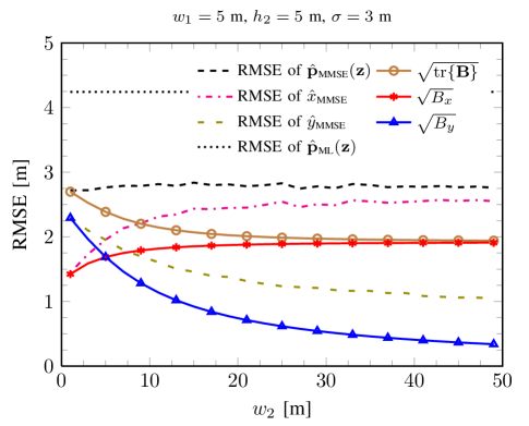
Figure 7: RMSE versus $w_{2}$ for the MMSE estimator (35). Map #2 (Fig. 2), $\sigma=3\,\text{m}$ and $\mathcal{A_{R}}=75\,\text{m}^{2}$ are assumed. The BCRB components $\sqrt{B_{x}}$, $\sqrt{B_{y}}$, $\sqrt{\operatorname{tr}\{\mathbf{B}\}}$ (see (32)) and the RMSE for the ML estimator are also shown for comparison.

IV-C Map #3

Observation model - Finally, let us analyse the RMSE performance of localization systems operating in the environment described by map #3 in two cases: A) the map-aware estimator knows map #3 exactly; B) the map-aware estimator assumes that the localization environment is described by the bounding box of map #3. Note that the last case is significant from a practical point of view, since, in the absence of detailed information about the floor of a building, the bounding box represents the best a priori model which can be adopted to describe the floor itself.
In addition, in this Paragraph model (2) is compared against a more specific counterpart, called “ranging observation model” in the following; for such modelling we assume that 1) the observations are acquired by 4 anchors placed in the map corners; 2) the observation provided by the $i$-th anchor can be expressed as

$$z_{i}=\left\|\mathbf{p}-\mathbf{p}_{i}^{a}\right\|+n_{i}$$ (36)

with $i=1,2,3,4$, where $n_{i}$ represents Gaussian noise with variance $\sigma^{2}$ and $\mathbf{p}_{i}^{a}$ represents the $i$-th anchor position.

The scenario considered in this example is helpful to assess 1) to what extent a detailed knowledge of the geometrical features of a map can improve localization accuracy with respect to the availability of a simplified map model (like a bounding box model) and 2) if a localization system based on the Gaussian model (2) can exhibit a similar behaviour as that of a localization system based on (36), at least in the considered cases.
Estimators - Given the model (36), the MAP estimator can be expressed as

$$\hat{\mathbf{p}}_{\text{\tiny{MAP}}}^{R}(\mathbf{z})=\arg\max_{\tilde{\mathbf{p}}\in\mathcal{R}}\mathcal{N}\left(\mathbf{z};\boldsymbol{\mu}(\tilde{\mathbf{p}}),\boldsymbol{\Sigma}^{R}\right)$$ (37)

where $\boldsymbol{\mu}(\mathbf{p})\triangleq\left[\left\|\mathbf{p}-\mathbf{p}_{1}^{a}\right\|,...,\left\|\mathbf{p}-\mathbf{p}_{4}^{a}\right\|\right]^{T}$ and $\boldsymbol{\Sigma}^{R}=\sigma^{2}\mathbf{I}_{4}$. If the observation model (2) is adopted in place of (36), the MAP estimator

$$\hat{\mathbf{p}}_{\text{\tiny{MAP}}}^{G}(\mathbf{z})=\arg\max_{\tilde{\mathbf{p}}\in\mathcal{R}}\mathcal{N}\left(\mathbf{z};\tilde{\mathbf{p}},\boldsymbol{\Sigma}^{G}\right)$$ (38)

is obtained, where $\boldsymbol{\Sigma}^{G}=\boldsymbol{\Sigma}=\sigma^{2}\mathbf{I}_{2}$.
Numerical results - Fig. 8 compares the RMSE performance achieved by the MAP estimators (37) and (38) versus $\sigma$ in cases A and B. These results show that:

1. Surprisingly the selection of the map model (map #3 in case A or its bounding box in case B) does not affect the MMSE estimation performance, whatever the model for the observations. This result can be motivated as follows. For each value of $\sigma$, there is some portion of the map where the combination of noise level and geometrical features (see the analysis of map #1) entails a large RMSE and where a detailed map (map #3) does not provide a substantial advantage over simpler maps (e.g., the bounding box); since the Bayesian RMSE results from an average of the agent position over the entire map, it is biased by such portions of the map for each value of $\sigma$. Such an effect influences also any global Bayesian bound, like the BCRB, the EZZB and the WWB: their values result from an average over the entire parameter space (in this case $\mathcal{R}$) and can be strongly influenced by the parameter values (in this case, the values of $\mathbf{p}$) characterized by the largest errors [37]. Note also that local bounds (e.g., CRB), which model the parameters to be estimated as deterministic variables, do not suffer from this problem, but cannot exploit a priori information and represent performance limits for unbiased estimators only [25]. In our case study a detailed knowledge of map #3 (case A) provides, in various subsets of $\mathcal{R}$, a substantial improvement with respect to the knowledge of the bounding box (case B), but the effects of such subsets are then “averaged out” when evaluating the Bayesian RMSE, as shown in Fig. 8.

2. The adoption of the Gaussian observation model (2) entails a worse accuracy than that provided by the ranging observation model (36). This can be related to the placement of the anchors and to their number; in fact, range observations coming from anchors displaced with a constant angular spacing allow to average out the measurement errors better than the positional observation of the Gaussian model (2) when the same noise variance $\sigma^{2}$ is assumed in both models. If the offset between the curves referring to the Gaussian and the ranging model is neglected, our results show that both curves exhibit the same behaviour, when $\sigma$ is varied; this is an hint to the fact that the insights obtained from the bounds derived for the model (2) may be useful also in the analysis of systems employing different observation models (like (36)).

Finally, comment 1) suggests that, when assessing the improvement in localization accuracy coming from map awareness, the evaluation of the overall RMSE does not provide sufficient information about the importance of a given map. In fact, if the effects of different portions of the maps are analysed, it is found that some of them play a more relevant role than other ones; in this perspective, the insights and the intuition acquired from the results referring to map #1 are very useful, given that map #1 can be thought of as a transversal slice of a subset of any 2-D map.

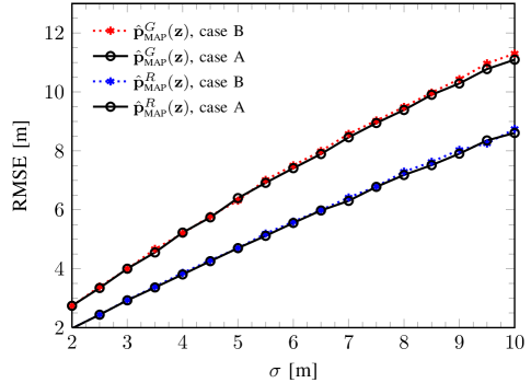
Figure 8: RMSE versus $\sigma$ for the MAP estimators (37) and (38), using either the Gaussian observation model (see (2)) or the ranging observation model (see (36)). The a priori map is map #3 (case A) or its bounding box (case B). The RMSE of ML estimators is also shown for comparison.

V Conclusion

In this manuscript the impact of map awareness on localization performance has been investigated from a theoretical perspective, evaluating different accuracy bounds. Such bounds provide some general indications about the role and importance of this form of a priori information. Our study has evidenced that, unluckily, the tighter is an accuracy bound, the more complicated is its dependence on the geometric parameters of maps. This has motivated the analysis of the developed bounds in specific environments; in particular, three different maps have been considered and, for each of them, the accuracy bounds have been evaluated and compared with the performance offered by map-aware and map-unaware estimators. Our analytical and numerical results have evidenced that: a) map-aware estimation accuracy can be related to some features of the map (e.g., its shape and area) even though, in general, the relation is complicated; b) maps are really useful in the presence of some combination of low SNRs and specific geometrical features of the map (e.g., the size of obstructions); c) for some combinations of SNRs and geometrical features, there is no need of refined maps since knowledge of map details provides only a negligible performance gain; d) in a given environment the EZZB and, in particular, the WWB are usually much tighter than the BCRB; e) in the cases of maps containing many features, the importance of map awareness is better captured by the analysis of subsets of those map.

Future improvements include the development of map-aware bounds for specific observation models; in particular models including bias due to the non-line of sight (NLOS) propagation may unveil important insights about map-aware localization systems operating in NLOS conditions.

Finally, it is important to point out that all the bounds derived in this manuscript can be also exploited for other estimation problems (provided that the vector of random parameters to be estimated is characterized by a uniform a priori pdf) and can be easily generalized to the case of estimation of an $N$-dimensional parameter vector, with $N>2$.

Appendix A Derivation of the BFIM and BCRB

In this Appendix the derivation of (8) and (11) is sketched. To begin, we consider a real function $s(t)$ having the following properties:

• it is continuous and differentiable;

• $s(t)\geq 0\>\forall t\in\mathbb{R}$;

• $\int s(t)dt=1$;

• $\int\frac{\partial s(t)}{\partial t}dt=0$;

• its support is the interval $\left[-1/2;1/2\right]$;

• $s(0)=1$.

These properties have the following implications: a) $s(t)$ is a pdf function (see P.1-P.3); b) an a-priori FI $\mathrm{J}_{s}$ can be computed for it (the regularity condition P.4 ensures the FI existence) [20]; c) $s(\cdot)$ can be used to model bounded statistical distributions (i.e., maps), eventually after some scaling and translation (see P.5, P.6). As far as the last point is concerned, it is worth mentioning that

$$\tilde{s}(t,a,b)\triangleq(1/b)\cdot s\left((t-a)/b\right)\>,$$

with $b>0$, is still a pdf function and its FI is $\tilde{\mathrm{J}}_{s}(b)=\mathrm{J}_{s}/b^{2}$. Any function $s(\cdot)$ sharing the properties P.1-P.6 represents a “smoothing function”; specific examples of smoothing functions can be found in [38].

Any smoothing function $s(t)$ can be used to define the analytical model of a smoothed uniform map. To show how this can be done, we start considering a unidimensional (1-D) scenario first, where the agent position to estimate is the scalar $x$. The support $\mathcal{R}\subset\mathbb{R}$ of a 1-D uniform map can be always represented as the union of $N_{r}$ disjoint segments spaced by $N_{r}-1$ segments where the map pdf $f(x)$ is equal to 0. Let the $N_{r}$ segments of the support $\mathcal{R}$ be indexed by the odd numbers of the set $\mathcal{N}^{o}=\{1,3,...,2N_{r}-1\}$ and let $c{}_{n}$ ($w{}_{n}$) denote the centre (width) of the $n$-th segment, with $n\in\mathcal{N}^{o}$. Then the map pdf $f(x)$ associated with this scenario can be expressed as

$$f(x)=\frac{1}{\mathcal{W_{R}}}\sum_{n\in\mathcal{N}^{o}}s\left(\frac{x-c_{n}}{w_{n}}\right)=\frac{1}{\mathcal{W_{R}}}\sum_{n\in\mathcal{N}^{o}}w_{n}\tilde{s}(x,c_{n},w_{n})$$ (39)

where $\mathcal{W_{R}}\triangleq\sum_{n\in\mathcal{N}^{o}}w_{n}$. The a priori FI associated with $f(x)$ is given by

$$\mathrm{J}_{x} \triangleq\mathbb{E}_{x}\left\{\left(\frac{\partial\ln f(x)}{\partial x}\right)^{2}\right\}$$

$$=\frac{1}{\mathcal{\mathcal{W_{R}}}}\sum_{n\in\mathcal{N}^{o}}w_{n}\mathbb{E}_{x}\left\{\left(\frac{\partial}{\partial x}\ln\tilde{s}(x,c_{n},w_{n})\right)^{2}\right\}$$

$$=\frac{1}{\mathcal{\mathcal{W_{R}}}}\sum_{n\in\mathcal{N}^{o}}w_{n}\tilde{\mathrm{J}}_{s}(w_{n})=\frac{1}{\mathcal{\mathcal{W_{R}}}}\sum_{n\in\mathcal{N}^{o}}\frac{\mathrm{J}_{s}}{w_{n}}$$ (40)

Let us extend these results to 2-D maps. Exploiting some definitions given in Section II and assuming that the smoothing along $x$ and that along $y$ are independent, the pdf for an arbitrary smoothed uniform 2-D map can be put in the form

$$f(\mathbf{p})=\frac{1}{\mathcal{\mathcal{A_{R}}}} \sum_{n\in\mathcal{N}_{h}^{o}(y)}s\left(\frac{x-c_{x,n}(y)}{w_{n}(y)}\right)\cdot$$

$$\sum_{m\in\mathcal{N}_{v}^{o}(x)}s\left(\frac{y-c_{y,m}(x)}{h_{m}(x)}\right)$$ (41)

where $c_{x,n}(y)$ ($c_{y,m}(x)$) and $w_{n}(y)$ ($h_{m}(x)$) denote the centre and the length, respectively of the $n$-th ($m$-th) segment. Let us now compute the elements of the BFIM $\mathbf{J}_{\mathbf{p}}$ associated with this pdf (see (6)). The analysis of (41) can be connected to that of (39) exploiting the formula (iterated expectation)

$$\left[\mathbf{J}_{\mathbf{p}}\right]_{1,1} \triangleq\mathbb{E}_{\mathbf{p}}\left\{\left(\frac{\partial\ln f(\mathbf{p})}{\partial x}\right)^{2}\right\}$$

$$=\mathbb{E}_{y}\left\{\mathbb{E}_{x|y}\left\{\left(\frac{\partial\ln f(\mathbf{p})}{\partial x}\right)^{2}\right\}\right\}$$ (42)

and adopting the approximation

$$f(\mathbf{p}) \simeq\frac{1}{\mathcal{\mathcal{A_{R}}}}\sum_{n\in\mathcal{N}_{h}^{o}(y)}s\left(\frac{x-c_{x,n}(y)}{w_{n}(y)}\right)$$ (43)

$$=\frac{\mathcal{W_{R}}(y)}{\mathcal{\mathcal{A_{R}}}}\frac{1}{\mathcal{\mathcal{W_{R}}}(y)}\sum_{n\in\mathcal{N}_{h}^{o}(y)}s\left(\frac{x-c_{x,n}(y)}{w_{n}(y)}\right)$$

where $\mathcal{\mathcal{W_{R}}}(y)\triangleq\sum_{n\in\mathcal{N}_{h}^{o}(y)}w_{n}(y)$. It is worth noting that in (43) the smoothing along the $y$ coordinate is ignored. This is a reasonable approximation whenever the smoothing only modifies a narrow area of the edges of $\mathcal{R}$ compared to the area of the flat regions of (41); the selection of a proper smoothing function ensures that such a condition holds (see Sec. II-A and [38]).
Thanks to (43), the evaluation of the inner expectation in (42) is equivalent to that of the FI referring to a 1-D map which consists of $N_{r}=N_{h}(y)$ segments having widths $\left\{w_{n}(y)\right\}$ and centred around the points $\left\{c_{x,n}(y)\right\}$; for this reason, from (39)-(40) it is easily inferred that

$$\mathbb{E}_{x|y}\left\{\left(\frac{\partial\ln f(\mathbf{p})}{\partial x}\right)^{2}\right\}\simeq\frac{\mathcal{\mathcal{\mathcal{W_{R}}}}(y)}{\mathcal{A_{R}}}\frac{\mathrm{J}_{s}}{\mathcal{\mathcal{\mathcal{W_{R}}}}(y)}\sum_{n\in\mathcal{N}_{h}^{o}(y)}\frac{1}{w_{n}(y)}$$ (44)

Substituting the last result in the RHS of (42) produces

$$\left[\mathbf{J}_{\mathbf{p}}\right]_{1,1} \simeq\frac{\mathrm{J}_{s}}{\mathcal{\mathcal{A_{R}}}}\int_{\mathcal{Y}}\sum_{n\in\mathcal{N}_{h}^{o}(y)}\frac{1}{w_{n}(y)}f(y)dy$$

$$\simeq\frac{\mathrm{J}_{s}}{\mathcal{\mathcal{A_{R}}}}\int_{\mathcal{Y}}\sum_{n\in\mathcal{N}_{h}^{o}(y)}\frac{dy}{w_{n}(y)}$$ (45)

where $f(y)\triangleq\int f(\mathbf{p})dx$ is the pdf of $y$ only and it has been ignored in the integral since the smoothing only affects a small portion of the integration domain (see Section II). A similar approach can be adopted in the evaluation of $\left[\mathbf{J}_{\mathbf{p}}\right]_{2,2}$ (ignoring, in this case, the smoothing along $x$); this leads to

$$\left[\mathbf{J}_{\mathbf{p}}\right]_{2,2}\simeq\frac{\mathrm{J}_{s}}{\mathcal{\mathcal{A_{R}}}}\int_{\mathcal{X}}\sum_{m\in\mathcal{N}_{v}^{o}(x)}\frac{1}{h_{m}(x)}dx$$ (46)

Note also that the approximated results (45)-(46) become exact if $\mathcal{R}$ is a rectangle having its sides parallel to the reference axes, since in this case the smoothing along $x$ is truly independent from the smoothing along $y$. For the same reason the cross terms $\left[\mathbf{J}_{\mathbf{p}}\right]_{2,1}$ and $\left[\mathbf{J}_{\mathbf{p}}\right]_{1,2}$ are exactly equal to zero for a rectangle; however since 2-D maps usually exhibit a weak correlation between the variables $x$ and $y$, these terms can be neglected; this leads to (8), from which (11) is easily obtained assuming that $\mathcal{N}_{h}^{e}(y)=\emptyset$ and $\mathcal{N}_{v}^{e}(x)=\emptyset$ $\forall x,y$.

Appendix B Derivation of the EZZB

In this Appendix the EZZB (13) is derived following a procedure conceptually similar to the one provided in [25, Sec. II.B]. We start from the identity (see [39, p. 24])

$$E_{\nu}=\frac{1}{2}\int_{0}^{\infty}\Pr\left\{\left|\xi_{\nu}\right|\geq\frac{h}{2}\right\}h\>dh$$ (47)

where $\xi_{\nu}\triangleq\left[\hat{\mathbf{p}}(\mathbf{z})-\mathbf{p}\right]_{\nu}$. Following [25], the probability appearing in (47) can be put in the form

$$\Pr\left\{\left|\xi_{\nu}\right|\geq\frac{h}{2}\right\} =\Pr\left\{\xi_{\nu}>\frac{h}{2}\right\}+\Pr\left\{\xi_{\nu}\leq-\frac{h}{2}\right\}$$

$$=\int_{\mathbb{R}^{N}}\Pr\left\{\xi_{\nu}>\frac{h}{2}|\mathbf{p}=\boldsymbol{\rho}_{0}\right\}f(\boldsymbol{\rho}_{0})d\boldsymbol{\rho}_{0}$$

$$+\int_{\mathbb{R}^{N}}\Pr\left\{\xi_{\nu}\leq-\frac{h}{2}|\mathbf{p}=\boldsymbol{\rho}_{1}\right\}f(\boldsymbol{\rho}_{1})d\boldsymbol{\rho}_{1}$$ (48)

where $f(\cdot)$ denotes the pdf of $\mathbf{p}$. Let $\boldsymbol{\rho}_{0}=\boldsymbol{\rho}$ and $\boldsymbol{\rho}_{1}=\boldsymbol{\rho}+\boldsymbol{\delta}(h)$, where $\boldsymbol{\delta}(h)$ is some function of the integration variable of (47). If the integration domain of (48) is constrained to be a subset $\mathcal{R}(h)$ of the map support $\mathcal{R}$, such that $f(\boldsymbol{\rho})>0$ and $f(\boldsymbol{\rho}+\boldsymbol{\delta}(h))>0$, then, dividing and multiplying the RHS of (48) by $f(\boldsymbol{\rho})+f(\boldsymbol{\rho}+\boldsymbol{\delta}(h))>0$, produces the expression [25, eqs. (22)-(30)]

$$\Pr\left\{\left|\xi_{\nu}\right|\geq\frac{h}{2}\right\}\geq\\ \int_{\mathcal{R}(h)}\left[f(\boldsymbol{\rho})+f(\boldsymbol{\rho}+\boldsymbol{\delta}(h))\right]P_{\text{\tiny{min}}}^{\mathbf{z}}(\boldsymbol{\rho},\boldsymbol{\rho}+\boldsymbol{\delta}(h))d\boldsymbol{\rho}$$ (49)

($P_{\text{\tiny{min}}}^{\mathbf{z}}(\boldsymbol{\rho},\boldsymbol{\rho}+\boldsymbol{\delta}(h))$ is defined in Sec. III-B) which holds for any $\boldsymbol{\delta}(h)$ satisfying the equality $\mathbf{a}^{T}\boldsymbol{\delta}(h)=h$, where $\mathbf{a}\in\mathbb{R}^{2}$. Note that (49) generalizes [25, eq. (30)] to the case where the pdf $f(\cdot)$ of the parameter to estimate has a bounded support. Here $\mathbf{a}=\mathbf{e}_{\nu}$ is selected so that $\boldsymbol{\delta}(h)=h\mathbf{e}_{\nu}$. Then substituting (49) in (47) produces (13), where the integration domains of $h$ and $\boldsymbol{\rho}$ have been merged in the set $\mathcal{P}_{\nu}$.

Like in the previous Appendix, let us evaluate now (13) for a 1-D uniform map whose support $\mathcal{R}\subset\mathbb{R}$ consists of the union of $N_{r}$ disjoint segments. In the following such segments are indexed by the odd numbers of the set $\mathcal{N}^{o}=\{1,3,...,2N_{r}-1\}$ and the lower (upper) limit of the segment $n\in\mathcal{N}^{o}$ is denoted $l_{n}\triangleq c_{n}-\frac{w_{n}}{2}$ ($u_{n}\triangleq c_{n}+\frac{w_{n}}{2}$), where $c{}_{n}$ ($w{}_{n}$) represents the centre (length) of the segment itself. Moreover, it is assumed, without any loss of generality, that $c_{1}<c_{3}<...<c_{2N_{r}-1}$. In this 1-D scenario (13) simplifies as

$$Z\triangleq\frac{1}{2}\iint_{\mathcal{P}}\left[f(\tau)+f(\tau+h)\right]P_{\text{\tiny{min}}}^{z}(\tau,\tau+h)h\,d\tau\>dh$$ (50)

where $\boldsymbol{\rho}=\tau$,

$$\mathcal{P}=\left\{(\tau,h):h\geq 0\wedge f(\tau)>0\wedge f(\tau+h)>0\right\}$$

and $P_{\text{\tiny{min}}}^{z}(\tau,\tau+h)$ represents the minimum error probability of a binary detector which, on the basis of a noisy datum $z$ and a likelihood ratio test, has to select one of the following two hypotheses $H_{0}:\>x=\tau$ and $H_{1}:\>x=\tau+h$. Note that, for any $(\tau,h)\in\mathcal{P}$, we have that $f(\tau)+f(\tau+h)=2/\mathcal{W_{\mathcal{R}}}$ (with $\mathcal{W_{\mathcal{R}}}\triangleq\sum_{n\in\mathcal{N}^{o}}w_{n}\vphantom{A_{A_{A_{A_{A}}}}}$), because of the uniformity of the considered map. If the Gaussian observation model (2) adopted to the 1-D case is assumed, the average error probability of the above mentioned detector is easily shown to be

$$P_{\text{\tiny{min}}}^{z}(\tau,\tau+h)=\frac{1}{2}\operatorname{erfc}\left(h/(2\sigma\sqrt{2})\right)$$

(where $\sigma$ denotes the standard deviation of the noise observation model), which is independent of $\tau$; then, (50) simplifies as

$$Z =\frac{1}{2\mathcal{\mathcal{W_{\mathcal{R}}}}}\iint_{\mathcal{P}}h\operatorname{erfc}\left(\frac{h}{2\sigma\sqrt{2}}\right)d\tau\>dh$$

$$=\frac{\sigma^{3}}{2\mathcal{\mathcal{W_{\mathcal{R}}}}}\iint_{\mathcal{Q}}u\operatorname{erfc}\left(\frac{u}{2\sqrt{2}}\right)dt\>du$$ (51)

where $u\triangleq h/\sigma$, $t\triangleq\tau/\sigma$ and

$$\mathcal{Q}\triangleq\left\{(t,u):u\geq 0\wedge f(\sigma t)>0\wedge f(\sigma(t+u))>0\right\}$$

can be shown to be 2-D domain consisting of the union of $N_{r}$ triangles and $N_{r}(N_{r}-1)/2$ parallelograms in the plane $(t,u)$, as exemplified by Fig. 9, which refers to the case $N_{r}=3$. In particular, the contribution to the RHS of (51) from the $i$-th triangle

$$\mathcal{Q}_{i}\triangleq\left\{(t,u):\frac{l_{i}}{\sigma}\leq t\leq\frac{u_{i}}{\sigma}\wedge 0\leq u\leq\frac{u_{i}}{\sigma}-t\right\}$$

can be shown to be $\sigma^{2}\zeta(\rho_{i})/(2\rho_{\mathcal{W}})$, where $\rho_{i}\triangleq w_{i}/\sigma$, $\rho_{\mathcal{W}}\triangleq\mathcal{W_{\mathcal{R}}}/\sigma$, the function $\zeta(\rho)$ is defined in (15) and $i\in\mathcal{N}^{o}$ (see [38] for more details). As far as the parallelograms are concerned, we retain only the contributions coming from $(N_{r}-1)$ parallelograms

$$\mathcal{Q}_{ov,i}\triangleq\left\{(t,u):\frac{l_{i}}{\sigma}\leq t\leq\frac{u_{i}}{\sigma}\right.\left.\wedge\frac{l_{i}}{\sigma}-t\leq u\leq\frac{u_{i}}{\sigma}-t\right\}$$

with $i\in\mathcal{N}^{e}\triangleq\{2,4,...,2(N_{r}-1)\}$ (see Fig. 9); such contributions are given by $\sigma^{2}\zeta_{ov}(\rho_{\triangle_{i}},\rho_{i-1},\rho_{i+1})/(2\rho_{\mathcal{W}})$, where $\rho_{\triangle_{i}}\triangleq\triangle x_{i}/\sigma$, $\triangle x_{i}\triangleq l_{i+1}-u_{i-1}$ and $\zeta_{ov}(\rho_{\triangle},\rho_{1},\rho_{2})$ is defined in (16) for $\rho_{1}>\rho_{2}$ (it can be shown that $\zeta_{ov}(\rho_{\triangle},\rho_{1},\rho_{2})=\zeta_{ov}(\rho_{\triangle},\rho_{2},\rho_{1})$). Note that the contributions to (51) coming from the discarded parallelograms are always positive since $u\operatorname{erfc}\left(\frac{u}{2\sqrt{2}}\right)\geq 0$ for $u\geq 0$. Then, substituting the above mentioned contributions in (51) produces the lower bound

$$Z>\frac{\sigma^{2}}{2\rho_{\mathcal{W}}}\left[\sum_{n\in\mathcal{N}^{o}}\zeta\left(\rho_{n}\right)+\sum_{n\in\mathcal{N}^{e}}\zeta_{ov}\left(\rho_{\triangle_{n}},\rho_{n-1},\rho_{n+1}\right)\right]$$ (52)

for the EZZB. The approach developed for a 1-D uniform map can be extended to a 2-D scenario keeping into account that a) the term $P_{\text{\tiny{min}}}^{\mathbf{z}}(\boldsymbol{\rho},\boldsymbol{\rho}+h\mathbf{e}_{\nu})$ of (13) takes on a similar form as $P_{\text{\tiny{min}}}^{z}(\tau,\tau+h)$ of (50), b) the integral on $\boldsymbol{\rho}$ can be decomposed in a couple of nested integrals, one over $\mathcal{X}$ and the other one over $\mathcal{Y}$, and c) eq. (52) can be exploited for the inner integral. Further details can be found in [38].

Appendix C Derivation of the WWB

In this Appendix we first derive the WWB for a $2$-D uniform map characterized by a support $\mathcal{R}$, assuming the observation model (2). Note that this derivation can be easily generalised to a $N$-D scenario. To begin, we note that, since $f(\mathbf{z}|\mathbf{p})=\mathcal{N}(\mathbf{z};\mathbf{p},\boldsymbol{\Sigma})$ (see (2)), the likelihood ratio $L\left(\mathbf{z};\mathbf{p}_{1},\mathbf{p}_{2}\right)$ (21) is given by $\mathcal{N}(\mathbf{z};\mathbf{p}_{1},\boldsymbol{\Sigma})/\mathcal{N}(\mathbf{z};\mathbf{p}_{2},\boldsymbol{\Sigma})$ $\forall\mathbf{p}_{1},\mathbf{p}_{2}\in\mathcal{R}$. Then, it is not difficult to prove that the expectation appearing in the numerator of (20) is given by

$$\mathbb{E}_{\mathbf{z},\mathbf{p}}\left\{L^{\frac{1}{2}}\left(\mathbf{z};\mathbf{p}+h_{\nu}\mathbf{e}_{\nu},\mathbf{p}\right)\right\}$$

$$=\frac{1}{\mathcal{A_{R}}}\int_{\mathbb{R}^{2}}\int_{\mathcal{P}_{\nu}(h_{\nu})}\negthickspace\mathcal{N}^{\frac{1}{2}}\left(\mathbf{z};\boldsymbol{\rho}+h_{\nu}\mathbf{e}_{\nu},\boldsymbol{\Sigma}\right)\mathcal{N}^{\frac{1}{2}}\left(\mathbf{z};\boldsymbol{\rho},\boldsymbol{\Sigma}\right)d\boldsymbol{\rho}\>d\mathbf{z}$$

$$=\frac{1}{\mathcal{A_{R}}}\exp\left(-\frac{h_{\nu}^{2}}{8\sigma_{\nu}^{2}}\right)\int_{\mathcal{P}_{\nu}(h_{\nu})}d\boldsymbol{\rho}$$ (53)

where $\mathcal{P}_{\nu}(h_{\nu})\triangleq\left\{\boldsymbol{\rho}:f(\boldsymbol{\rho})>0\wedge f(\boldsymbol{\rho}+h_{\nu}\mathbf{e}_{\nu})>0\right\}$ is a slice of the integration domain $\mathcal{P}_{\nu}\subset\mathbb{R}^{3}$ involved in the evaluation of the EZZB [38] and $\nu\in\{x,y\}$. The expectation appearing in the denominator of (19) can be expressed as

$$\mathbb{E}_{\mathbf{z},\mathbf{p}}\left\{\left[L^{\frac{1}{2}}\left(\mathbf{z};\mathbf{p}+h_{\nu}\mathbf{e}_{\nu},\mathbf{p}\right)-L^{\frac{1}{2}}\left(\mathbf{z};\mathbf{p}-h_{\nu}\mathbf{e}_{\nu},\mathbf{p}\right)\right]^{2}\right\}\\ =\mathbb{E}_{\mathbf{z},\mathbf{p}}\left\{L\left(\mathbf{z};\mathbf{p}+h_{\nu}\mathbf{e}_{\nu},\mathbf{p}\right)\right\}+\mathbb{E}_{\mathbf{z},\mathbf{p}}\left\{L\left(\mathbf{z};\mathbf{p}-h_{\nu}\mathbf{e}_{\nu},\mathbf{p}\right)\right\}\\ -2\cdot\mathbb{E}_{\mathbf{z},\mathbf{p}}\left\{L^{\frac{1}{2}}\left(\mathbf{z};\mathbf{p}+h_{\nu}\mathbf{e}_{\nu},\mathbf{p}\right)L^{\frac{1}{2}}\left(\mathbf{z};\mathbf{p}-h_{\nu}\mathbf{e}_{\nu},\mathbf{p}\right)\right\}$$

i.e., as the sum of three terms which are denoted $A$, $B$ and $C$, respectively, in the following. It is important to note that

$$A =\mathbb{E}_{\mathbf{z},\mathbf{p}}\left\{L\left(\mathbf{z};\mathbf{p}+h_{\nu}\mathbf{e}_{\nu},\mathbf{p}\right)\right\}$$

$$=\frac{1}{\mathcal{A_{R}}}\int_{\mathbb{R}^{2}}\int_{\mathcal{P}_{\nu}(h_{\nu})}\mathcal{N}(\mathbf{z};\boldsymbol{\rho}+h_{\nu}\mathbf{e}_{\nu},\boldsymbol{\Sigma})d\boldsymbol{\rho}d\mathbf{z}$$

$$=\frac{1}{\mathcal{A_{R}}}\int_{\mathcal{P}_{\nu}(h_{\nu})}d\boldsymbol{\rho}=\frac{1}{\mathcal{A_{R}}}\lambda_{\nu}\left(h_{\nu},\mathcal{R}\right)$$

$$=\mathbb{E}_{\mathbf{z},\mathbf{p}}\left\{L\left(\mathbf{z};\mathbf{p}-h_{\nu}\mathbf{e}_{\nu},\mathbf{p}\right)\right\}$$

$$=B$$ (54)

and

$$C =\frac{1}{\mathcal{A_{R}}}\int_{\mathbb{R}^{2}}\int_{\tilde{\mathcal{P}}_{\nu}(h_{\nu})}\mathcal{N}(\mathbf{z};\boldsymbol{\rho}+h_{\nu}\mathbf{e}_{\nu},\boldsymbol{\Sigma})d\boldsymbol{\rho}d\mathbf{z}$$

$$=\frac{1}{\mathcal{A_{R}}}\exp\left(-\frac{h_{\nu}^{2}}{2\sigma_{\nu}^{2}}\right)\int_{\tilde{\mathcal{P}}_{\nu}(h_{\nu})}d\boldsymbol{\rho}$$

$$=\frac{1}{\mathcal{A_{R}}}\exp\left(-\frac{h_{\nu}^{2}}{2\sigma_{\nu}^{2}}\right)\gamma_{\nu}\left(h_{\nu},\mathcal{R}\right)$$ (55)

where

$$\tilde{\mathcal{P}}_{\nu}(h_{\nu})\triangleq\left\{\boldsymbol{\rho}:f(\boldsymbol{\rho})>0\right. \wedge f(\boldsymbol{\rho}+h\mathbf{e}_{\nu})>0$$

$$\left.\wedge f(\boldsymbol{\rho}-h\mathbf{e}_{\nu})>0\right\}$$

and the functions $\lambda_{\nu}\left(h_{\nu},\mathcal{R}\right)$ and $\gamma_{\nu}\left(h_{\nu},\mathcal{R}\right)$ are defined in (23) and (24). Then, substituting (53), (54), (55) in (20) produces (22).

Finally, it is worth pointing out that $\lambda_{\nu}\left(h_{\nu},\mathcal{R}\right)$ (23) and $\gamma_{\nu}\left(h_{\nu},\mathcal{R}\right)$ (24) can be explicitly related to the functions $\left\{w_{n}(\cdot)\right\}$, $\left\{\triangle w_{n}(\cdot)\right\}$, $\left\{h_{m}(\cdot)\right\}$, $\left\{\triangle h_{m}(\cdot)\right\}$ introduced in Section II. To clarify this point, let us focus on $\lambda_{x}\left(h_{x},\mathcal{R}\right)$ and $\gamma_{x}\left(h_{x},\mathcal{R}\right)$ which can be derived, for a given ordinate $y$, analysing the integration domain

$$\mathcal{P}_{x}(h_{x},y)\triangleq\left\{\tau:f(\tau,y)>0\wedge f(\tau+h_{x},y)>0\right\}\>.$$

If the variables $t\triangleq\tau/\sigma$ and $u\triangleq h_{x}/\sigma$ are defined, this domain can be put in the form

$$\mathcal{Q}_{x}(u,y)=\left\{t:f(\sigma t,y)>0\wedge f(\sigma(t+u),y)>0\right\}\>,$$

which describes a slice of the $(t,u)$ plane of Fig. 9. The contribution of the $i$-th triangle $\mathcal{Q}_{i}$ to $\lambda_{x}(h_{x},\mathcal{R}(y))$ ($\gamma_{x}(h_{x},\mathcal{R}(y))$) is given by $\omega\left(w_{i}(y),h_{x}\right)$ ($\omega_{ov}\left(\triangle w_{i}(y),w_{i-1}(y),w_{i+1}(y),h_{x}\right)$), where $\omega(w_{n}(y),h_{x})$ is defined in (25), $\omega_{ov}\left(\triangle w,w_{1},w_{2},h\right)$ is defined in (26) and $\mathcal{R}(y)$ is the slice of the map support $\mathcal{R}$ at the ordinate $y$. Similarly, the contribution from the $i$-th parallelogram $\mathcal{Q}_{ov,i}$ to $\lambda_{x}\left(h_{x},\mathcal{R}(y)\right)$ is given by $\omega_{ov}\left(\triangle w_{i}(y),w_{i-1}(y),w_{i+1}(y),h_{x}\right)$. Therefore, the overall contribution to $\lambda_{x}(h_{x},\mathcal{R}(y))$ can be expressed as

$$\sum_{n\in\mathcal{N}_{h}^{o}(y)}\omega\left(w_{n}(y),h_{x}\right)+\\ \sum_{n\in\mathcal{N}_{h}^{e}(y)}\omega_{ov}\left(\triangle w_{n}(y),w_{n-1}(y),w_{n+1}(y),h_{x}\right)$$ (56)

whereas that to $\gamma_{x}(h_{x},\mathcal{R}(y))$ as

$$2\sum_{n\in\mathcal{N}_{h}^{o}(y)}\omega\left(\frac{1}{2}w_{n}(y),h_{x}\right)$$ (57)

Finally, integrating (56) and (57) produces (23) and (24), respectively.

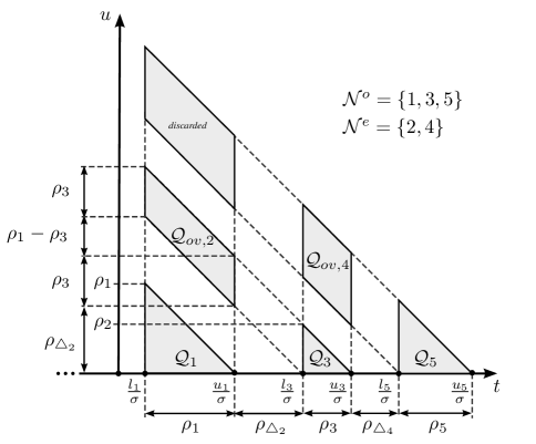
Figure 9: Representation of the set $\mathcal{Q}$ and of its subsets $\left\{\mathcal{Q}_{i}\right\}_{i\in\mathcal{N}^{o}}$ and $\left\{\mathcal{Q}_{ov,i}\right\}_{i\in\mathcal{N}^{e}}$ in the $(t,u)$ plane ($N_{r}=3$ is assumed). Note that the contribution from the “discarded” parallelogram is neglected in the evaluation of both (24)-(23) and (51).

Francesco Montorsi (S’06) received both the Laurea degree (cum laude) and the Laurea Specialistica degree (cum laude) in Electronic Engineering from the University of Modena and Reggio Emilia, Italy, in 2007 and 2009, respectively. He received the Ph.D degree in Information and Communications Technologies (ICT) from the University of Modena and Reggio Emilia in 2013. He is employed as embedded system engineer for an ICT company since 2013. In 2011 he was a visiting PhD student at the Wireless Communications and Network Science Laboratory of Massachusetts Institute of Technology (MIT). His research interests are in the area of localization and navigation systems, with emphasis on statistical signal processing (linear and non-linear filtering, detection and estimation problems), model-based design and model-based performance assessment. Dr. Montorsi is a member of IEEE Communications Society and served as a reviewer for the IEEE Transactions on Wireless Communications, IEEE Transactions on Signal Processing, IEEE Wireless Communications Letters and several IEEE conferences.

Santiago Mazuelas (M’10) received his Ph.D. in mathematics and Ph.D. in telecommunications engineering from the University of Valladolid, Spain, in 2009 and 2011, respectively. Since 2009, he has been a postdoctoral fellow in the Wireless Communication and Network Sciences Laboratory at MIT. He previously worked from 2006 to 2009 as a researcher and project manager in a Spanish technological center, as well as a junior lecturer in the University of Valladolid. His research interests are the application of mathematical and statistical theories to communications, localization, and navigation networks. Dr. Mazuelas has served as a member of the Technical Program Committee (TPC) for the IEEE Global Communications Conference (GLOBECOM) in 2010, 2011, and 2012, the IEEE International Conference on Ultra-Wideband (ICUWB) in 2011, the 75th IEEE Vehicular Technology Conference 2012, and the IEEE Wireless Telecommunications Symposium (WTS) in 2010 and 2011. He has received the 2012 IEEE Communications Society Fred W. Ellersick Prize, the Best Paper Award from the IEEE GLOBECOM in 2011, the Best Paper Award from the IEEE ICUWB in 2011, and the young scientists prize for the best communication at the Union Radio-Scientifique Internationale (URSI) XXII Symposium in 2007.

Giorgio M. Vitetta (S’89-M’91-SM’99) was born in Reggio Calabria, Italy, in April 1966. He received the Dr. Ing. degree in electronic engineering (cum laude) in 1990, and the Ph.D. degree in 1994, both from the University of Pisa, Pisa, Italy. From 1995 to 1998, he was a Research Fellow with the Department of Information Engineering, University of Pisa. From 1998 to 2001, he was an Associate Professor with the University of Modena and Reggio Emilia, Modena, Italy, where he is currently a full Professor. His main research interests lie in the broad area of communication theory, with particular emphasis on detection/equalization/synchronization algorithms for wireless communications, statistical modelling of wireless and powerline channels, ultrawideband communication techniques and applications of game theory to wireless communications. Dr. Vitetta is serving as an Editor of the IEEE Wireless Communications Letters and as an Area Editor of the IEEE Transactions on Communications.

Moe Z. Win (S’85-M’87-SM’97-F’04) received both the Ph.D. in Electrical Engineering and M.S. in Applied Mathematics as a Presidential Fellow at the University of Southern California (USC) in 1998. He received an M.S. in Electrical Engineering from USC in 1989, and a B.S. (magna cum laude) in Electrical Engineering from Texas A&M University in 1987. He is a Professor at the Massachusetts Institute of Technology (MIT). Prior to joining MIT, he was at AT&T Research Laboratories for five years and at the Jet Propulsion Laboratory for seven years. His research encompasses fundamental theories, algorithm design, and experimentation for a broad range of real-world problems. His current research topics include network localization and navigation, network interference exploitation, intrinsic wireless secrecy, adaptive diversity techniques, and ultra-wide bandwidth systems. Professor Win is an elected Fellow of the AAAS, the IEEE, and the IET, and was an IEEE Distinguished Lecturer. He was honored with two IEEE Technical Field Awards: the IEEE Kiyo Tomiyasu Award (2011) and the IEEE Eric E. Sumner Award (2006, jointly with R. A. Scholtz). Together with students and colleagues, his papers have received numerous awards including the IEEE Communications Society’s Stephen O. Rice Prize (2012), the IEEE Aerospace and Electronic Systems Society’s M. Barry Carlton Award (2011), the IEEE Communications Society’s Guglielmo Marconi Prize Paper Award (2008), and the IEEE Antennas and Propagation Society’s Sergei A. Schelkunoff Transactions Prize Paper Award (2003). Highlights of his international scholarly initiatives are the Copernicus Fellowship (2011), the Royal Academy of Engineering Distinguished Visiting Fellowship (2009), and the Fulbright Fellowship (2004). Other recognitions include the Laurea Honoris Causa from the University of Ferrara (2008), the Technical Recognition Award of the IEEE ComSoc Radio Communications Committee (2008), and the U.S. Presidential Early Career Award for Scientists and Engineers (2004). Dr. Win is an elected Member-at-Large on the IEEE Communications Society Board of Governors (2011–2013). He was the chair (2004–2006) and secretary (2002–2004) for the Radio Communications Committee of the IEEE Communications Society. Over the last decade, he has organized and chaired numerous international conferences. He is currently an Editor-at-Large for the IEEE Wireless Communications Letters, and serving on the Editorial Advisory Board for the IEEE Transactions on Wireless Communications. He served as Editor (2006–2012) for the IEEE Transactions on Wireless Communications, and served as Area Editor (2003–2006) and Editor (1998–2006) for the IEEE Transactions on Communications. He was Guest-Editor for the Proceedings of the IEEE (2009) and IEEE Journal on Selected Areas in Communications (2002).

References

- [1] K. Pahlavan and J. Makela, “Indoor geolocation science and technology,” IEEE Commun. Mag., vol. 40, no. 2, pp. 112–118, Feb. 2002.
- [2] M. Z. Win, W. M. Gifford, S. Mazuelas, Y. Shen, D. Dardari, and M. Chiani, “Network Localization and Navigation via Cooperation,” IEEE Commun. Mag., vol. 49, no. 5, pp. 56–62, May 2011.
- [3] Y. Qi and H. Kobayashi, “On geolocation accuracy with prior information in non-line-of-sight environment,” in Proc. of IEEE Veh. Technology Conference, Birmingham, AL, 2002, pp. 285–288.
- [4] E. Larsson, “Cramer-Rao Bound Analysis of Distributed Positioning in Sensor Networks,” IEEE Signal Process. Lett., vol. 11, no. 3, pp. 334–337, Mar. 2004.
- [5] F. Gustafsson and F. Gunnarsson, “Mobile positioning using wireless networks: possibilities and fundamental limitations based on available wireless network measurements,” IEEE Signal Process. Mag., vol. 22, no. 4, pp. 41 – 53, Jul. 2005.
- [6] Y. Qi, H. Kobayashi, and H. Suda, “Analysis of wireless geolocation in a non-line-of-sight environment,” IEEE Trans. Wireless Commun., vol. 5, no. 3, pp. 672–681, Mar. 2006.
- [7] S. Gezici, Z. Tian, G. Giannakis, H. Kobayashi, A. Molisch, H. Poor, and Z. Sahinoglu, “Localization via ultra-wideband radios: a look at positioning aspects for future sensor networks,” IEEE Signal Process. Mag., vol. 22, no. 4, pp. 70–84, Jul. 2005.
- [8] S. Gezici and H. Poor, “Position Estimation via Ultra-Wide-Band Signals,” Proc. IEEE, vol. 97, no. 2, pp. 386–403, Feb. 2009.
- [9] Y. Shen and M. Z. Win, “On the Accuracy of Localization Systems Using Wideband Antenna Arrays,” IEEE Trans. on Commun., vol. 58, no. 1, pp. 270–280, Jan. 2010.
- [10] ——, “Fundamental Limits of Wideband Localization - Part I: A General Framework,” IEEE Trans. on Inf. Theory, vol. 56, no. 10, pp. 4956–4980, Oct. 2010.
- [11] N. Patwari, J. Ash, S. Kyperountas, A. O. Hero, III, R. Moses, and N. Correal, “Locating the nodes: cooperative localization in wireless sensor networks,” IEEE Signal Process. Mag., vol. 22, no. 4, pp. 54–69, Jul. 2005.
- [12] Y. Shen, H. Wymeersch, and M. Z. Win, “Fundamental Limits of Wideband Localization - Part II: Cooperative Networks,” IEEE Trans. on Inf. Theory, vol. 56, no. 10, pp. 4981–5000, Oct. 2010.
- [13] S. Mazuelas, Y. Shen, and M. Z. Win, “Information Coupling in Cooperative Localization,” IEEE Commun. Lett., vol. 15, no. 7, pp. 737–739, Jul. 2011.
- [14] Y. Cheng and T. Singh, “Efficient Particle Filtering for Road-Constrained Target Tracking,” IEEE Trans. Aerosp. Electron. Syst., vol. 43, no. 4, pp. 1454–1469, Oct. 2007.
- [15] S. Beauregard, Widyawan, and M. Klepal, “Indoor PDR Performance Enhancement using Minimal Map Information and Particle Filters,” in IEEE/ION Position, Location and Navigation Symp., Monterey, CA, 2008, pp. 141–147.
- [16] P. Davidson, J. Collin, and J. Takala, “Application of Particle Filters for Indoor Positioning Using Floor Plans,” in Proc. Ubiquitous Positioning Indoor Navigation and Location Based Service Conf., Kirkkonummi, 2010, pp. 1–4.
- [17] D. Anzai and S. Hara, “An Area Layout-based MAP Estimation for Indoor Target Tracking,” in IEEE Veh. Technol. Conf., Ottawa, ON, 2010, pp. 1–5.
- [18] M. Anisetti, C. A. Ardagna, V. Bellandi, E. Damiani, and S. Reale, “Map-Based Location and Tracking in Multipath Outdoor Mobile Networks,” IEEE Trans. on Wireless Commun., vol. 10, no. 3, pp. 814–824, Mar. 2011.
- [19] H. L. V. Trees, Detection, Estimation and Modulation Theory, Part III: Radar-Sonar Processing and Gaussian Signals in Noise. John Wiley & Sons, Inc, 2001.
- [20] S. Kay, Fundamentals of Statistical Signal Processing: Estimation Theory. Prentice Hall, 1993, vol. I.
- [21] R. E. Kass and L. Wasserman, “The Selection of Prior Distributions by Formal Rules,” J. of the Amer. Statistical Association, vol. 91, no. 435, pp. 1343–1370, Sep. 1996.
- [22] L. Seidman, “Performance limitations and error calculations for parameter estimation,” Proc. of the IEEE, vol. 58, no. 5, pp. 644–652, May 1970.
- [23] D. Chazan, M. Zakai, and J. Ziv, “Improved Lower Bounds on Signal Parameter Estimation,” IEEE Trans. on Inf. Theory, vol. 21, no. 1, pp. 90–93, Jan. 1975.
- [24] J. Ziv and M. Zakai, “Some Lower Bounds on Signal Parameter Estimation,” IEEE Trans. on Inf. Theory, vol. 15, no. 3, pp. 386–391, May 1969.
- [25] K. Bell, Y. Steinberg, Y. Ephraim, and H. L. Van Trees, “Extended Ziv-Zakai Lower Bound for Vector Parameter Estimation,” IEEE Trans. on Inf. Theory, vol. 43, no. 2, pp. 624–637, Mar. 1997.
- [26] D. Nicholson and A. Vecchio, “Bayesian bounds on parameter estimation accuracy for compact coalescing binary gravitational wave signals,” Physical Review D, vol. 57, no. 8, pp. 4588–4599, Apr. 1998.
- [27] F. Montorsi and G. M. Vitetta, “On the Performance Limits of Pilot-Based Estimation of Bandlimited Frequency-Selective Communication Channels,” IEEE Trans. on Commun., vol. 59, no. 11, pp. 2964–2969, Nov. 2011.
- [28] A. J. Weiss and E. Weinstein, “A Lower Bound on the Mean-Square Error in Random Parameter Estimation,” IEEE Trans. on Inf. Theory, vol. 31, no. 5, pp. 680–682, Sep. 1985.
- [29] Z. Ben-Haim and Y. C. Eldar, “A Comment on the Weiss-Weinstein Bound for Constrained Parameter Sets,” IEEE Trans. on Inf. Theory, vol. 54, no. 10, pp. 4682–4684, Oct. 2008.
- [30] S. Chaiken, D. J. Kleitman, M. Saks, and J. Shearer, “Covering regions by rectangles,” SIAM J. Alg. Disc. Meth., vol. 2, no. 4, pp. 394–410, 1981.
- [31] W. Liou, J.-M. Tan, and R. Lee, “Minimum rectangular partition problem for simple rectilinear polygons,” IEEE Trans. Comput.-Aided Des. Integr. Circuits Syst., vol. 9, no. 7, pp. 720–733, Jul. 1990.
- [32] S.-Y. Wu and S. Sahni, “Fast Algorithms to Partition Simple Rectilinear Polygons,” VLSI Design, vol. 1, no. 3, pp. 193–215, 1994.
- [33] P. Vandewalle, J. Kovacevic, and M. Vetterli, “Reproducible Research in Signal Processing - What, why, and how,” IEEE Signal Process. Mag., vol. 26, no. 3, pp. 37–47, May 2009.
- [34] S. Mazuelas, A. Bahillo, R. M. Lorenzo, P. Fernandez, F. a. Lago, E. Garcia, J. Blas, and E. J. Abril, “Robust Indoor Positioning Provided by Real-Time RSSI Values in Unmodified WLAN Networks,” IEEE J. Sel. Topics Signal Process., vol. 3, no. 5, pp. 821–831, Oct. 2009.
- [35] P. Pivato, L. Palopoli, and D. Petri, “Accuracy of RSS-Based Centroid Localization Algorithms in an Indoor Environment,” IEEE Trans. Instrum. Meas., vol. 60, no. 10, pp. 3451–3460, Oct. 2011.
- [36] H. Liu, H. Darabi, P. Banerjee, and J. Liu, “Survey of Wireless Indoor Positioning Techniques and Systems,” IEEE Trans. Syst. Man Cybern. C, Appl. Rev., vol. 37, no. 6, pp. 1067–1080, Nov. 2007.
- [37] T. Routtenberg and J. Tabrikian, “A General Class of Outage Error Probability Lower Bounds in Bayesian Parameter Estimation,” IEEE Trans. on Signal Process., vol. 60, no. 5, pp. 2152–2166, May 2012.
- [38] F. Montorsi and G. M. Vitetta, “Technical Report: Detailed Proofs of Bounds for Map-Aware Localization,” University of Modena and Reggio Emilia, Tech. Rep., 2012, available online at http://frm.users.sourceforge.net/publications.html.
- [39] E. Cinlar, Introduction to Stochastic Processes. Prentice-Hall, 1975.