$WW\gamma/Z$ production in the Randall-Sundrum model at the LHC and CLIC

Abstract

We study the $W^{+}W^{-}\gamma(Z)$ productions at both the CERN Large Hadron Collider (LHC) and the Compact Linear Collider (CLIC) in the framework of the Randall-Sundrum (RS) model. The impacts of the virtual RS Kaluza-Klein (KK) graviton on these processes are studied and compared with the standard model (SM) background. We present the integrated and differential cross sections in both the RS model and the SM. The results show that the relative RS discrepancies at the CLIC differ from those at the LHC, particularly in the transverse momentum and rapidity distributions. We also find that the RS signature performance, as a result of the resonance character of the RS KK-graviton spectrum, is distinctively unlike that in the large extra dimensions model. We conclude that the CLIC with unprecedented precision and high center-of-mass energy has a potential advantage over the LHC in exploring the effects of the RS KK graviton on the $W^{+}W^{-}\gamma(Z)$ production processes.

PACS: 11.10.Kk, 14.70.Fm, 14.70.Hp

I. INTRODUCTION

Solving the huge disparity between the Planck scale $M_{P}$ and the electroweak scale $M_{EW}$, which is known as the gauge hierarchy problem, has long been the motivation for proposing new physics beyond the standard model (SM). Strikingly distinct from the supersymmetry or technicolor models, the extra dimensions models, including the large extra dimensions (LED) [1] model with factorizable geometry and the Randall-Sundrum (RS) [2] model with nonfactorizable (warped) geometry, provide alternative solutions to the gauge hierarchy problem by postulating that the quantum gravity effects appear at the TeV scale, which may induce rich collider phenomena at the CERN Large Hadron Collider (LHC) and the future Compact Linear Collider (CLIC) [3].

In the LED model [1], we have $D=(4+n)$-dimensional spacetime with $n$ being the number of extra dimensions compactified on a $n$-dimensional torus with radius $R$, and the gauge hierarchy problem is solved via the relation $M_{P}\sim R^{n/2}M_{D}^{n/2+1}$ if $R$ is large enough. However, there appears a new hierarchy between the $D$-dimensional fundamental scale $M_{D}\sim 1$ TeV and the compactification radius $R^{-1}\sim$ eV-MeV in the LED molel, which motivates proposing the RS model. The RS model is based on a compactified warped extra dimension and two $3$-branes in the background of the $\textrm{AdS}_{5}$ spacetime. In the RS model, the gauge hierarchy problem is solved by an exponential warp factor. The RS Kaluza-Klein (KK) graviton spectrum shares distinct properties compared with that in the LED model, which has inspired many works on the phenomenological studies in the RS model, for example, the works on $pp\to VV,~{}\bar{l}l,~{}\bar{t}t$ [4]-[6], $e^{+}e^{-},pp\to G_{KK}G_{KK}$ [7], and $e^{+}e^{-},pp\to\bar{l}l\gamma$ [8].

The triple gauge boson (TGB) productions are of particular interest because they not only are sensitive to the quartic gauge couplings (QGCs) but also could demonstrate new physics signatures [9]. Any deviation from the SM predictions would hint at the existence of new physics, such as the non-SM electroweak symmetry breaking mechanism or the extra dimensions signals [10]. In this sense, the studies on the TGB production channels in extra dimensions models, including the LED model and the RS model, are necessary. Up to now, the TGB productions have been thoroughly studied in the SM [11], and the TGB production studies in the LED model have also received impressive attention in the literature, including the neutral TGB production processes $pp\to\gamma\gamma\gamma$, $pp\to\gamma\gamma Z$, $pp\to\gamma ZZ$ and $pp\to ZZZ$ in Ref.[12], $e^{+}e^{-}\to ZZZ$ at the CLIC in Ref.[13], and $e^{+}e^{-},pp\to W^{+}W^{-}\gamma/Z$ at the LHC and ILC in Ref.[14]. In the RS model, only the TGB production process $pp\to\gamma\gamma\gamma$ has been studied in Ref.[15].

In the present paper, we consider the effects of the virtual RS KK-graviton exchange on the $W^{+}W^{-}\gamma$ and $W^{+}W^{-}Z$ productions at both the LHC and the CLIC. Three areas of interest motivate this work. First, the $W^{+}W^{-}\gamma$ and $W^{+}W^{-}Z$ productions are excellent probes of the SM QGCs. Second, and different from the LED model, the fact that the RS KK-graviton spectrum generally manifests itself as TeV-order resonances could alter the cross sections and thus lead to identifiable changes in the TGB phenomenology at the LHC and the multi-TeV CLIC. Third, compared with the current data for QGCs available from LEP II and Tevatron [16], the LHC can provide more precise measurements of the QGCs due to its high energy and luminosity [17], and the multi-TeV CLIC can probe the QGCs with unprecedented precision due to the cleaner environment arising from $e^{+}e^{-}$ collisions and the compelling high energy [18]. Therefore, it can be expected that the LHC and the future multi-TeV CLIC will provide complementary studies on the TGB productions. The rest of the paper is organized as follows. In Sec.II, we briefly describe the related theory of the RS model. In Sec.III, the calculation strategy is presented. We perform the numerical analyses for the $W^{+}W^{-}\gamma$ and $W^{+}W^{-}Z$ productions at both colliders in Sec.IV. Section V is devoted to a short summary. In the Appendix, we present the relevant Feynman rules for vertices of the RS KK graviton coupled with the SM fields.

II. RELATED THEORY

In the brane-bulk scenario of the RS model [2], the spacetime is assumed to be $5=(4+1)$-dimensional with the one-dimensional extra dimension compactified on an $S_{1}/Z_{2}$ orbifold with radius $R_{c}$, and two $3$-branes, the Planck brane and TeV brane, reside at the orbifold fixed points $\phi=0,~{}\pi$, respectively. The five-dimensional bulk connecting the two branes is a slice of the $\textrm{AdS}_{5}$ spacetime, which is nonfactorizable and has a constant negative curvature. The nonfactorizable bulk metric is given by

$$ds^{2}=e^{-{\cal K}R_{c}\phi}\eta_{\mu\nu}dx^{\mu}dx^{\nu}~{}+~{}R_{c}^{2}d\phi^{2},$$ (2.1)

where $0\leq\phi\leq\pi$, and ${\cal K}$ is the curvature scale of the bulk. It is assumed that the SM fields are located at the TeV brane, while the gravity can propagate in the whole five-dimensional bulk. The Planck scale $M_{P}$ for gravity can be suppressed to the TeV scale via the exponential warp factor $e^{-\pi{\cal K}R_{c}}$, i.e., $M_{P}e^{-\pi{\cal K}R_{c}}\sim{\cal O}({\rm TeV})$ and thus the gauge hierarchy problem is solved. In the low-energy effective four-dimensional theory view, after taking a linear expansion of the gravity field as fluctuations around the flat metric and adopting the KK reduction [19], we obtain the interactions between the KK tower of massive spin-2 gravitons and the SM particles as

$${\cal L}=-{1\over\overline{M}_{P}}T^{\mu\nu}(x)G_{KK,\mu\nu}^{(0)}(x)-{1\over\Lambda_{\pi}}T^{\mu\nu}(x)\sum_{n=1}^{\infty}G_{KK,\mu\nu}^{(n)}(x),$$ (2.2)

where $\overline{M}_{P}=M_{P}/\sqrt{8\pi}$ is the reduced Planck scale and $T^{\mu\nu}$ is the energy-momentum tensor of the SM particles. The interactions between the zero mode of the RS KK graviton and the SM particles are suppressed by $\overline{M}_{P}$ and thus decouple, while the couplings of the massive RS KK graviton are suppressed by $\Lambda_{\pi}=e^{-\pi{\cal K}R_{c}}\overline{M}_{P}\sim$TeV. The mass of the $n$th RS KK graviton $G_{KK,\mu\nu}^{(n)}$ is

$$M_{n}=x_{n}{\cal K}~{}e^{-\pi{\cal K}R_{c}}={x_{n}\over x_{1}}M_{1},$$ (2.3)

where $x_{n}$ are roots of the equation of Bessel function $J_{1}(x)$, i.e., $J_{1}(x_{n})=0$. For example, the first three roots are $x_{1}\simeq 3.83$, $x_{2}\simeq 7.02$, and $x_{3}\simeq 10.17$. That shows the masses of the RS KK gravitons are unevenly spaced with the mass splitting of TeV order if $M_{1}\sim{\rm TeV}$.

The two independent input parameters in the RS model are chosen as

$$M_{1}=x_{1}{\cal K}e^{-\pi{\cal K}R_{c}},~{}~{}~{}~{}~{}c_{0}={\cal K}/\overline{M}_{P},$$ (2.4)

where $M_{1}$ is the mass of the first RS KK graviton and $c_{0}$ is the effective coupling. The theoretical requirements [19, 20] constrain $c_{0}$ in the range of $0.01\leq c_{0}\leq 0.1$. The Feynman rules for the RS model can be read off from the counterparts in the LED model [21] upon the replacement of [8, 19, 22]

$${\kappa\over 2}\to{1\over\Lambda_{\pi}}={c_{0}\over M_{1}}x_{1},$$ (2.5)

where $\kappa={2\over\overline{M}_{P}}$ is the gravitational coupling strength in the LED model [21]. We present the explicit expressions of the vertex Feynman rules in the RS model related to our calculations in the Appendix. The spin-2 RS KK-graviton propagator in the de Donder gauge can be expressed as

$$\tilde{G}_{\rm KK}^{\mu\nu\alpha\beta}=\frac{1}{2}D(\hat{s})\left[\eta^{\mu\alpha}\eta^{\nu\beta}+\eta^{\mu\beta}\eta^{\nu\alpha}-\frac{2}{1+2}\eta^{\mu\nu}\eta^{\alpha\beta}\right],$$ (2.6)

where the summation over the tower of the KK graviton is

$$D(\hat{s})=\sum_{n=1}^{\infty}\frac{i}{\hat{s}-M_{n}^{2}+iM_{n}\Gamma_{n}}.$$ (2.7)

The total decay width of the $n$th KK graviton can be expressed as [6, 22]

$$\Gamma_{n}={1\over 8\pi}x_{n}^{2}M_{n}c_{0}^{2}\Delta_{n},$$ (2.8)

and

$$\Delta_{n}=\Delta_{n}^{\gamma\gamma}+\Delta_{n}^{gg}+\Delta_{n}^{WW}+\Delta_{n}^{ZZ}+\sum_{\nu}\Delta_{n}^{\nu\nu}+\sum_{l}\Delta_{n}^{ll}+\sum_{q}\Delta_{n}^{qq}+\Delta_{n}^{HH},$$ (2.9)

where $\Delta_{n}^{yy}$ is a numerical coefficient for the decay $G^{(n)}_{KK}(x)\to yy$, and $y$ is the SM particle involved. The explicit values for $\Delta_{n}^{yy}$ are given in Refs.[6, 8, 21].

From Eqs.(2.2) and (2.7), one can find that all the massive RS KK gravitons should be considered and summed over. Howerver, the contributions of the higher modes of the massive KK gravitons are negligible due to the fact that the higher zeros of the Bessel function $J_{1}(x)$ generate heavier RS KK gravitons with masses of several TeV [22]. For simplicity, we consider only the lightest RS KK graviton ($n=1$) resonance which provides the dominant contribution [8, 23].

III. CALCULATION STRATEGY

The calculation strategy in this section is similar with that in Ref.[14]. The $pp\to W^{+}W^{-}\gamma,W^{+}W^{-}Z$ processes at the LHC include two kinds of subprocesses: the quark-antiquark annihilation and the gluon-gluon fusion, which are denoted as

$$~{}~{}~{}q(p_{1})+\bar{q}(p_{2})\to W^{+}(p_{3})+W^{-}(p_{4})+V(p_{5}),~{}~{}~{}~{}~{}~{}~{}~{}~{}~{}~{}~{}~{}~{}~{}~{}~{}$$ (3.1)

$$g(p_{1})+g(p_{2})\to W^{+}(p_{3})+W^{-}(p_{4})+V(p_{5}),~{}~{}~{}~{}~{}~{}~{}~{}~{}~{}~{}~{}~{}~{}~{}~{}~{}$$ (3.2)

where $q=u,d,s,c,b$ and $V=\gamma,Z$. The $e^{+}e^{-}\to W^{+}W^{-}\gamma,W^{+}W^{-}Z$ processes at the CLIC can be denoted as

$$e^{+}(p_{1})+e^{-}(p_{2})\to W^{+}(p_{3})+W^{-}(p_{4})+V(p_{5}),~{}~{}~{}~{}(V=\gamma,Z).$$ (3.3)

In reactions (3.1), (3.2) and (3.3), $p_{i}$ $(i=1,2,3,4,5)$ are the four-momenta of the incoming and outgoing particles. The leading order (LO) Feynman diagrams with RS KK-graviton exchange for the partonic processes (3.1) and (3.2) are depicted in Figs.1 and 2, respectively, while the LO non-SM-like Feynman diagrams in the RS model for the process (3.3) are depicted in Fig.3.

From the Feynman diagrams shown in Figs.1-3, one can find that the RS KK graviton couples not only to the fermion pair ($f\bar{f}G_{KK}$), vector boson pair ($VVG_{KK}$), and fermion-antifermion-vector boson ($f\bar{f}VG_{KK}$) but also to the TGB vertices ($VVVG_{KK}$), which is similar to the case in the LED model [14]. In this sense, it is natural to expect that the RS KK graviton with mass of TeV order may induce considerably distinctive effects on the TGB production processes at the LHC and the future multi-TeV CLIC.

Figure 1: The LO Feynman diagrams for the partonic process $q\bar{q}\to W^{+}W^{-}\gamma/Z~{}(q=u,d,s,c,b)$ with KK-graviton exchange in the RS model. The SM-like diagrams are not shown.

Figure 2: The LO Feynman diagrams for the gluon-gluon fusion subprocess $gg\to W^{+}W^{-}\gamma/Z$ with KK-graviton exchange in the RS model.

Figure 3: The LO Feynman diagrams for the $e^{+}e^{-}\to W^{+}W^{-}\gamma/Z$ process with KK-graviton exchange in the RS model. The SM-like diagrams are not shown.

We express the Feynman amplitudes for the subprocesses $q\bar{q}\to W^{+}W^{-}\gamma/Z$ $(q=u,d,c,s,b)$ and $gg\to W^{+}W^{-}\gamma/Z$ as

$${\cal M}_{q\bar{q}}^{\gamma/Z}={\cal M}_{q\bar{q}}^{\gamma/Z,SM}+{\cal M}_{q\bar{q}}^{\gamma/Z,RS},~{}~{}~{}~{}{\cal M}_{gg}^{\gamma/Z}={\cal M}_{gg}^{\gamma/Z,RS},$$ (3.4)

where ${\cal M}_{q\bar{q}}^{\gamma/Z,SM}$ stands for the amplitude contributed by the SM-like diagrams, while ${\cal M}_{q\bar{q}}^{\gamma/Z,RS}$ and ${\cal M}_{gg}^{\gamma/Z,RS}$ are the amplitudes contributed by the diagrams with virtual RS KK-graviton exchange. The Feynman amplitude for the $e^{+}e^{-}\to W^{+}W^{-}\gamma/Z$ process can be separated into two components,

$${\cal M}_{ee}^{\gamma/Z}={\cal M}_{ee}^{\gamma/Z,SM}+{\cal M}_{ee}^{\gamma/Z,RS},$$ (3.5)

where ${\cal M}_{ee}^{\gamma/Z,SM}$ and ${\cal M}_{ee}^{\gamma/Z,RS}$ represent the amplitudes of the SM-like and the RS KK-graviton exchange diagrams, respectively.

The total cross sections for the partonic processes $q\bar{q}(gg)\to W^{+}W^{-}\gamma/Z$ have the form

$$\hat{\sigma}_{ij}^{\gamma/Z}=\frac{1}{4|\vec{p}|\sqrt{\hat{s}}}\int{\rm d}\Gamma_{3}\sum_{spin}^{color}{}^{\prime}|{\cal M}_{ij}^{\gamma/Z}|^{2},~{}~{}~{}~{}(ij=u\bar{u},d\bar{d},c\bar{c},s\bar{s},b\bar{b},gg),$$ (3.6)

where $\vec{p}$ is the three-momentum of one initial parton in the center-of-mass system (c.m.s), the summation is taken over the spins and colors of the initial and final states, and the prime on the sum denotes averaging over the initial spins and colors. The three-body phase space element ${\rm d}\Gamma_{3}$ is defined as

$${\rm d}\Gamma_{3}=(2\pi)^{4}\delta^{(4)}\left(p_{1}+p_{2}-\sum_{i=3}^{5}p_{i}\right)\prod_{i=3}^{5}\frac{d^{3}\vec{p}_{i}}{(2\pi)^{3}2E_{i}}.$$ (3.7)

The total cross sections for the $pp\to W^{+}W^{-}\gamma/Z$ processes at the hadronic level are obtained by convoluting $\hat{\sigma}^{\gamma/Z}_{ij}$ with the parton distribution functions (PDFs) of the colliding protons in the following way,

$$\sigma_{pp}^{\gamma/Z}=\sum^{c\bar{c},b\bar{b},gg}_{ij=u\bar{u},d\bar{d},s\bar{s}}\frac{1}{1+\delta_{ij}}\int dx_{A}dx_{B}\left[G_{i/A}(x_{A},\mu_{f})G_{j/B}(x_{B},\mu_{f})\hat{\sigma}^{\gamma/Z}_{ij}(\sqrt{\hat{s}}=x_{A}x_{B}\sqrt{s})+(A\leftrightarrow B)\right],$$

where $G_{i/P}$ $(i=q,\bar{q},g,P=A,B)$ represents the PDF of parton $i$ in proton $P(=A,B)$, $\mu_{f}$ is the factorization scale, and $x_{A}$ and $x_{B}$ refer to the momentum fractions of the parton (quark or gluon) in protons $A$ and $B$, respectively. The total cross sections for $e^{+}e^{-}\to W^{+}W^{-}\gamma(Z)$ can be expressed as

$$\sigma_{ee}^{\gamma/Z} = \frac{1}{4|\vec{p}|\sqrt{s}}\int{\rm d}\Gamma_{3}\sum_{spin}{}^{\prime}|{\cal M}_{ee}^{\gamma/Z}|^{2},$$ (3.9)

where $\vec{p}$ is the three-momentum of the incoming $e^{+}$ (or $e^{-}$) in the c.m.s of the $e^{+}e^{-}$ collider. The prime on the sum means averaging over the initial spin states as declared for Eq.(3.6).

IV. NUMERICAL RESULTS AND DISCUSSIONS

In this section we present the numerical results and the kinematic distributions for the $W^{+}W^{-}\gamma$ and $W^{+}W^{-}Z$ productions in both the SM and the RS model at the LHC and the CLIC. For the computations at the LHC, we use the CTEQ6L1 PDFs [24] with $\Lambda_{QCD}=165$ MeV and $n_{f}=5$ and take the factorization scale as $\mu_{f}=m_{W}$ and $\mu_{f}=m_{W}+m_{Z}/2$ for the $pp\to W^{+}W^{-}\gamma$ and $pp\to W^{+}W^{-}Z$ processes, respectively. The masses of the active quarks are neglected, i.e., $m_{q}=0~{}(q=u,d,c,s,b)$, and the CKM matrix is set to be the unit matrix. The other relevant input parameters are chosen as [25]

$$~{}~{}~{}~{}~{}~{}\alpha^{-1}(0)=137.036,~{}~{}m_{W}=80.385~{}\textrm{GeV},~{}~{}m_{Z}=91.1876~{}\textrm{GeV},$$

$$M_{H}=125~{}\textrm{GeV},~{}~{}m_{t}=173.5~{}\textrm{GeV},~{}~{}m_{e}=0.511\times 10^{-3}~{}\textrm{GeV}.$$ (4.1)

For the $e^{+}e^{-}/pp\to W^{+}W^{-}\gamma$ processes we apply a transverse momentum cut $p_{T}^{\gamma}>25$ GeV and a rapidity cut $|\eta^{\gamma}|<2.7$ on the final photon in order to remove the infrared (IR) singularity at the tree level.

Recently, the dilepton searches at ATLAS have excluded at the $95\%$ confidence level the RS KK graviton with masses below $2.16$ TeV [26]. The diphoton experiments at ATLAS provided $95\%$ confidence level lower limits on the lightest RS KK-graviton mass $M_{1}$ [27]: $1.03$ TeV for $c_{0}=0.01$, and $2.23$ TeV for $c_{0}=0.1$. In the present paper, we choose $M_{1}=2.25$ TeV and $c_{0}=0.1$ unless otherwise stated.

In Figs.4 and 5, we depict the transverse momentum ($p_{T}$) distributions of final $W^{-}$, $\gamma$ and $Z$ for the $e^{+}e^{-}\to W^{+}W^{-}\gamma,W^{+}W^{-}Z$ processes at the $\sqrt{s}=5$ TeV CLIC, respectively. Figures 6 and 7 show the $p_{T}^{W^{-}}$, $p_{T}^{\gamma}$ and $p_{T}^{Z}$ distributions for the processes $pp\to W^{+}W^{-}\gamma,W^{+}W^{-}Z$ at the $\sqrt{s}=14$ TeV LHC. In each plot of Figs.4-7, we provide $p_{T}^{W^{-}}$, $p_{T}^{\gamma}$ and $p_{T}^{Z}$ distributions in both the SM and the RS model for comparison. We define the relative RS discrepancy of $p_{T}$ distribution as $\delta(p_{T})\equiv\left(\frac{d\sigma_{RS}}{dp_{T}}-\frac{d\sigma_{SM}}{dp_{T}}\right)/\frac{d\sigma_{SM}}{dp_{T}}$ to describe the virtual RS KK-graviton effect, and plot the corresponding $\delta(p_{T})$ distribution in the nether plot for each figure. From Fig.4 we find that at the CLIC both $\delta(p_{T}^{W^{-}})$ and $\delta(p_{T}^{\gamma})$ for the $e^{+}e^{-}\to W^{+}W^{-}\gamma$ process lie in the negative range, which means that the RS KK-graviton mediated processes attenuate the SM background in the $p_{T}$ region of $25$ GeV $\leq p_{T}\leq 250$ GeV. The curves of $\delta(p_{T}^{W^{-}})$ and $\delta(p_{T}^{Z})$ for the $e^{+}e^{-}\to W^{+}W^{-}Z$ process behave in a similar way as the former process. Figures 6 and 7 show that the RS effect at the LHC enhances the SM contributions in the same region, and the relative discrepancies $\delta(p_{T}^{W^{-}})$, $\delta(p_{T}^{\gamma})$ and $\delta(p_{T}^{Z})$ at the LHC become larger with the increment of $p_{T}$. The distinct characteristic of the $p_{T}$ distributions at the CLIC and the LHC can serve as the complementary study on the TGB production events.

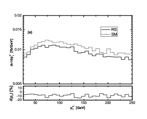
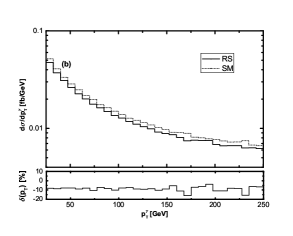
Figure 4: The transverse momentum distributions of the final $W^{-}$ and $\gamma$ and the corresponding relative RS discrepancies for the $e^{+}e^{-}\to W^{+}W^{-}\gamma$ process at the $\sqrt{s}=5$ TeV CLIC, with the RS parameters $M_{1}=2.25$ TeV and $c_{0}=0.1$. (a) for $p_{T}^{W^{-}}$, (b) for $p_{T}^{\gamma}$.

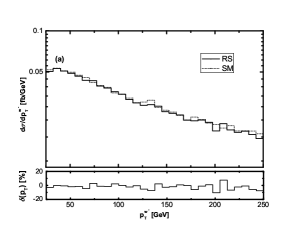
Figure 5: The transverse momentum distributions of the final $W^{-}$ and $Z$ and the corresponding relative RS discrepancies for the $e^{+}e^{-}\to W^{+}W^{-}Z$ process at the $\sqrt{s}=5$ TeV CLIC, with the RS parameters $M_{1}=2.25$ TeV and $c_{0}=0.1$. (a) for $p_{T}^{W^{-}}$, (b) for $p_{T}^{Z}$.

Figure 6: The transverse momentum distributions of the final $W^{-}$ and $\gamma$ and the corresponding relative RS discrepancies for the $pp\to W^{+}W^{-}\gamma$ process at the $\sqrt{s}=14$ TeV LHC, with the RS parameters $M_{1}=2.25$ TeV and $c_{0}=0.1$. (a) for $p_{T}^{W^{-}}$, (b) for $p_{T}^{\gamma}$.

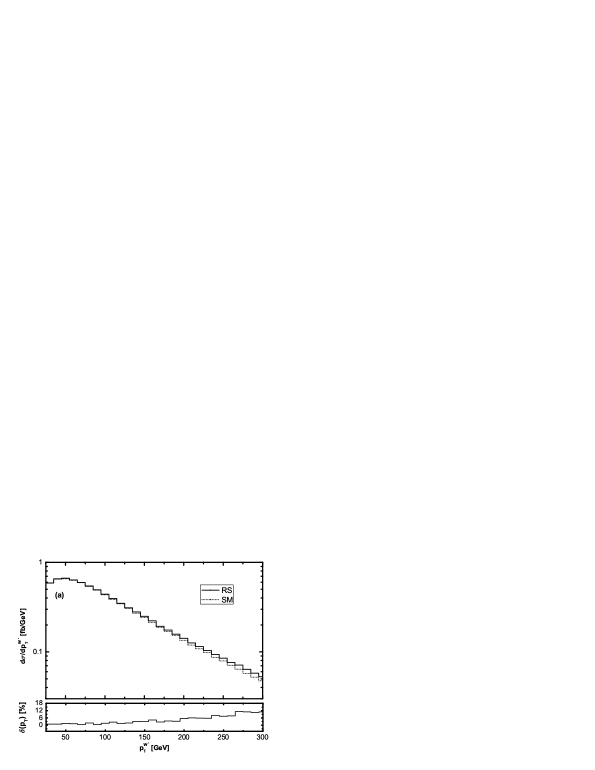
Figure 7: The transverse momentum distributions of the final $W^{-}$ and $Z$ and the corresponding relative RS discrepancies for the $pp\to W^{+}W^{-}Z$ process at the $\sqrt{s}=14$ TeV LHC, with the RS parameters $M_{1}=2.25$ TeV and $c_{0}=0.1$. (a) for $p_{T}^{W^{-}}$, (b) for $p_{T}^{Z}$.

In Figs.8 and 9, we present the rapidity ($y$) distributions of the final $W$ pair, $\gamma$ and $Z$ boson for the $e^{+}e^{-}\to W^{+}W^{-}\gamma,W^{+}W^{-}Z$ processes at the $\sqrt{s}=5$ TeV CLIC. In each plot of Figs.8-9, the $y^{WW}$, $y^{\gamma}$ and $y^{Z}$ distributions are given in both the SM and the RS model for comparison, and the corresponding relative RS discrepancies, defined as $\delta(y)\equiv\left(\frac{d\sigma_{RS}}{dy}-\frac{d\sigma_{SM}}{dy}\right)/\frac{d\sigma_{SM}}{dy}$, are depicted in each nether plot. They show that the curves of $\delta(y^{WW})$ at the CLIC are quite different from the corresponding results at the ILC in the LED model presented in Ref.[14] due to the RS KK-graviton resonance effects. The $\delta(y^{WW})$ distributions at the CLIC depicted in Figs.8(a) and 9(a) reach the same maximum value of about $50\%$ at the positions of $y^{WW}\sim\pm 0.78$. In addition, $\delta(y^{\gamma})$ in Fig.8(b) reaches its maximum (minimum) value about $12\%$ ($-12\%$) at $y^{\gamma}\sim 0$ ($y^{\gamma}\sim\pm 1.0$), and $\delta(y^{Z})$ in Fig.9(b) achieves its maximum (minimum) value of of about $19\%$ ($-14\%$) at $y^{Z}\sim 0$ ($y^{Z}\sim\pm 1.4$).

The $y^{WW}$, $y^{\gamma}$ and $y^{Z}$ distributions of the $pp\to W^{+}W^{-}\gamma,W^{+}W^{-}Z$ processes in the SM and the RS model at the $\sqrt{s}=14$ TeV LHC are shown in Figs.10 and 11, separately. There we also provide the corresponding relative RS discrepancies depicted in each nether plot. From the figures we can see that the line shapes of the relative RS discrepancies at the LHC differ from those at the CLIC, and the variations of $\delta(y^{WW})$, $\delta(y^{\gamma})$ and $\delta(y^{Z})$ at the LHC are milder than the corresponding ones at the CLIC shown in Figs.8 and 9.

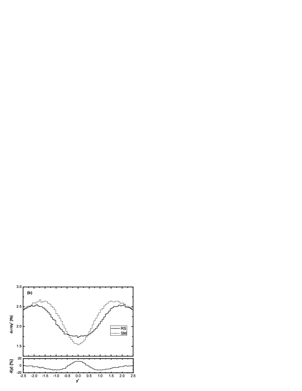
Figure 8: The rapidity distributions of the final $W$ pair and $\gamma$ and the corresponding relative RS discrepancies for the $e^{+}e^{-}\to W^{+}W^{-}\gamma$ process in both the SM and the RS model at the $\sqrt{s}=5$ TeV CLIC, with the RS parameters $M_{1}=2.25$ TeV and $c_{0}=0.1$, (a) for $y^{WW}$. (b) for $y^{\gamma}$.

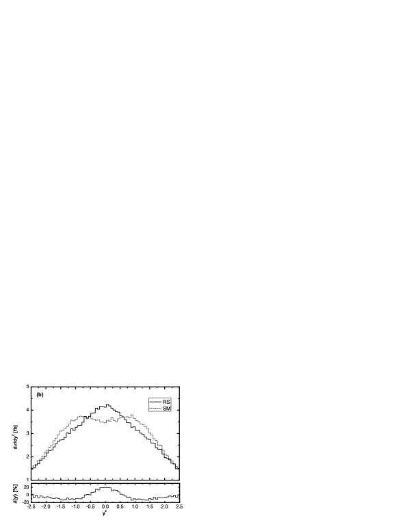
Figure 9: The rapidity distributions of final $W$ pair and $Z$ and the corresponding relative RS discrepancies for the $e^{+}e^{-}\to W^{+}W^{-}Z$ process in both the SM and the RS model at the $\sqrt{s}=5$ TeV CLIC, with the RS parameters $M_{1}=2.25$ TeV and $c_{0}=0.1$. (a) for $y^{WW}$, (b) for $y^{Z}$.

Figure 10: The rapidity distributions of final $W$ pair and $\gamma$ and the corresponding relative RS discrepancies for the $pp\to W^{+}W^{-}\gamma$ process in both the SM and the RS model at the $\sqrt{s}=14$ TeV LHC, with the RS parameters $M_{1}=2.25$ TeV and $c_{0}=0.1$. (a) for $y^{WW}$, (b) for $y^{\gamma}$.

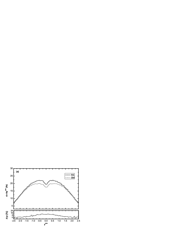
Figure 11: The rapidity distributions of final $W$ pair and $Z$ and the corresponding relative RS discrepancies for the $pp\to W^{+}W^{-}Z$ process in both the SM and the RS model at the $\sqrt{s}=14$ TeV LHC, with the RS parameters $M_{1}=2.25$ TeV and $c_{0}=0.1$. (a) for $y^{WW}$, (b) for $y^{Z}$.

In Figs.12 and 13, we present the $W$-pair invariant mass ($M_{WW}$) distributions in both the SM and the RS model at the $\sqrt{s}=5$ TeV CLIC and $\sqrt{s}=14$ TeV LHC, respectively. In Figs.14(a) and 14(b), the $W^{+}W^{-}\gamma/Z$ invariant mass ($M_{WW\gamma/Z}$) distributions for the $pp\to W^{+}W^{-}\gamma,W^{+}W^{-}Z$ processes at the LHC are depicted, separately. In each plot of Figs.12-14, the peaks on the solid curves indicate the existence of the RS KK graviton. We can see that the RS resonances appear at the locations of $M_{WW}\simeq M_{1}=2.25$ TeV in Figs.12-13 and $M_{WW\gamma/Z}\simeq M_{1}=2.25$ TeV in Fig.14, where $M_{1}=2.25$ TeV is the mass of the lightest RS KK graviton. Figs.12-14 show that the spin-2 RS KK graviton, which couples not only with the $W$ pair but also with the $W^{+}W^{-}\gamma(Z)$ vertices, contributes dominantly over the SM component in the RS KK-graviton resonance region, which is the character of the RS model and definitely differs from the results in the LED model [14].

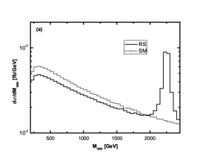
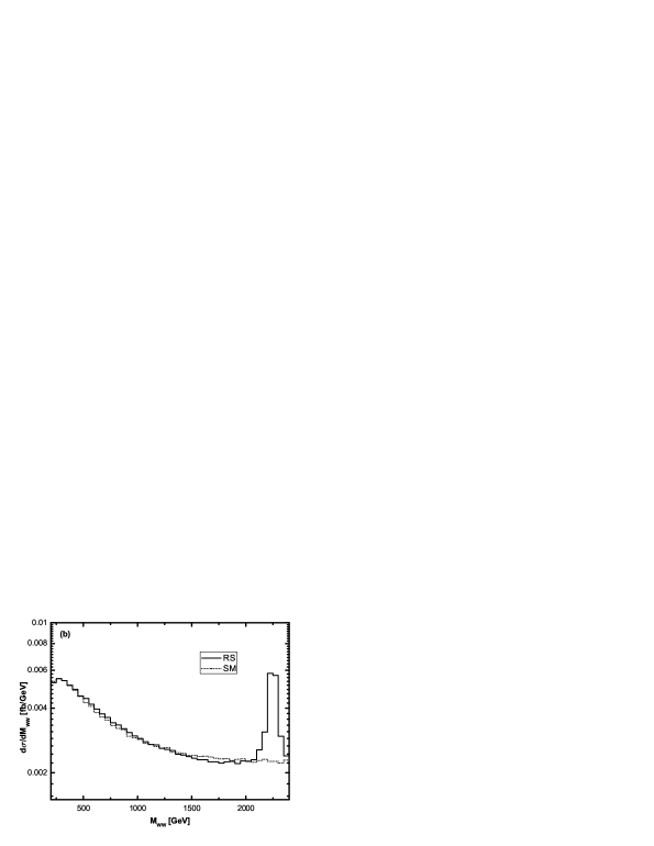
Figure 12: $M_{WW}$ distributions in both the SM and the RS model at the $\sqrt{s}=5$ TeV CLIC, with the RS parameters $M_{1}=2.25$ TeV and $c_{0}=0.1$. (a) for the $e^{+}e^{-}\to W^{+}W^{-}\gamma$ process, (b) for the $e^{+}e^{-}\to W^{+}W^{-}Z$ process.

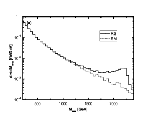
Figure 13: $M_{WW}$ distributions in both the SM and the RS model at the $\sqrt{s}=14$ TeV LHC, with the RS parameters $M_{1}=2.25$ TeV and $c_{0}=0.1$. (a) for the $pp\to W^{+}W^{-}\gamma$ process, (b) for the $pp\to W^{+}W^{-}Z$ process.

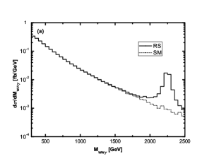
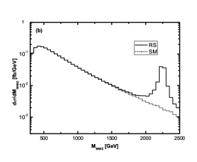
Figure 14: $M_{WW\gamma(Z)}$ distributions in both the SM and the RS model at the $\sqrt{s}=14$ TeV LHC, with the RS parameters $M_{1}=2.25$ TeV and $c_{0}=0.1$. (a) for the $pp\to W^{+}W^{-}\gamma$ process, (b) for the $pp\to W^{+}W^{-}Z$ process.

In Figs.15 and 16, we present the integrated cross sections as functions of the c.m.s energy $\sqrt{s}$ at the CLIC and the LHC, respectively. From Figs.15(a) and 15(b) we find that the integrated cross sections at the CLIC in both the SM and the RS model decrease as $\sqrt{s}$ becomes larger, and there exists an RS KK-graviton resonance peak on each curve for the $e^{+}e^{-}\to W^{+}W^{-}\gamma,W^{+}W^{-}Z$ processes in the RS model at the position of $\sqrt{s}\simeq M_{1}=2.25$ TeV. By contrast, the curves in Fig.16 for the $pp\to W^{+}W^{-}\gamma,W^{+}W^{-}Z$ processes at the LHC in both the SM and RS model increase with the increment of $\sqrt{s}$, and there is no appearance of the RS resonance peak due to the convolution of the PDFs.

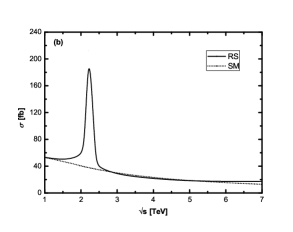
Figure 15: The integrated cross sections as functions of the c.m.s energy $\sqrt{s}$ in both the SM and the RS model at the CLIC, with the RS parameters $M_{1}=2.25$ TeV and $c_{0}=0.1$. (a) for the $e^{+}e^{-}\to W^{+}W^{-}\gamma$ process, (b) for the $e^{+}e^{-}\to W^{+}W^{-}Z$ process.

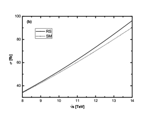
Figure 16: The integrated cross sections as functions of the c.m.s energy $\sqrt{s}$ in both the SM and the RS model at the LHC, with the RS parameters $M_{1}=2.25$ TeV and $c_{0}=0.1$. (a) for the $pp\to W^{+}W^{-}\gamma$ process, (b) for the $pp\to W^{+}W^{-}Z$ process.

In Figs.17 and 18, we show the relations between the integrated cross sections and the RS parameter $M_{1}$ with $c_{0}=0.03,0.05,0.07$ and $0.1$, in the $W^{+}W^{-}\gamma(Z)$ production processes at the CLIC and LHC, respectively. The horizon line in each plot stands for the SM cross section, which is independent of $M_{1}$ and $c_{0}$. Compared with the obscure behaviors of $\sigma(M_{1},c_{0})$ at the CLIC shown in Fig.17, the cross sections for the $pp\to W^{+}W^{-}\gamma,W^{+}W^{-}Z$ processes in Fig.18 exhibit more monotone relationship with the increment of the RS parameter $M_{1}$ or $c_{0}$. Figure.18 shows when the value of $M_{1}$ is fixed, we see the larger the value of $c_{0}$, the more evident the deviation due to the large RS KK-graviton contributions. In addition, it shows $\sigma(M_{1},c_{0})$ decreases and gradually approaches the SM results with the increment of $M_{1}$.

Figure 17: The integrated cross sections as functions of $M_{1}$ with $c_{0}=0.03,0.05,0.07$ and $0.1$ at the $\sqrt{s}=5$ TeV CLIC. The SM results appear as the straight lines. (a) for the $e^{+}e^{-}\to W^{+}W^{-}\gamma$ process, (b) for the $e^{+}e^{-}\to W^{+}W^{-}Z$ process.

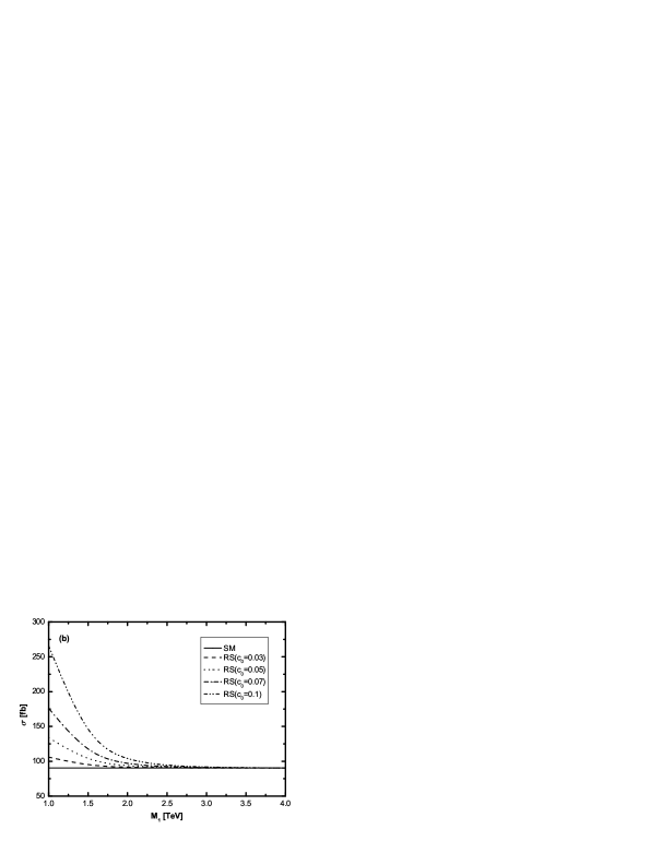
Figure 18: The integrated cross sections as functions of $M_{1}$ with $c_{0}=0.03,0.05,0.07$ and $0.1$ at the $\sqrt{s}=14$ TeV LHC. The SM results appear as the straight lines. (a) for the $pp\to W^{+}W^{-}\gamma$ process, (b) for the $pp\to W^{+}W^{-}Z$ process.

From the above discussion we can see that the kinematical observables for the $W^{+}W^{-}\gamma(Z)$ production processes at the CLIC and LHC have generally different behaviors, and the resonance effects of the RS KK graviton at both colliders are also dissimilar to those in the LED model shown in Ref.[14]. This difference can be ascribed to the following distinct features of the RS KK-graviton spectrum [22]: (1) In the LED model the multiplicity of the LED KK-graviton density collectively contributes to arrive at the electroweak scale, while the coupling of the RS KK graviton with the SM particles individually reaches the electroweak strength via the enhancement of the warp factor $e^{\pi{\cal K}R_{c}}$. (2) The LED KK-graviton spectrum is closely spaced with mass separation $\Delta m\sim{\cal O}(1/R)<0.1$ GeV leading to form a quasicontinuum, which manifests itself as a nonresonance contribution. Comparatively, the spectrum of the RS KK graviton is widely spaced with mass splitting of TeV order, and can possibly make the RS KK graviton being produced as resonance at the LHC and the CLIC.

V. SUMMARY

In this paper, we study the effects of the virtual RS KK graviton on the $W^{+}W^{-}\gamma$ and $W^{+}W^{-}Z$ productions at the LHC and the CLIC. The SM background is also included for comparison. We find that the transverse momentum ($p_{T}$) distributions and the corresponding RS relative discrepancies $\delta(p_{T})$ at the CLIC and the LHC exhibit opposite behaviors, namely, the RS KK-graviton effects tend to eliminate the SM contributions at the CLIC, but enhance them at the LHC. We provide the rapidity distributions ($y$) of the final particles, and it is shown that the RS relative discrepancies $\delta(y)$ at the LHC differ from those at the CLIC, and the $\delta(y)$ distribution shapes are unlike those in the LED model [14]. The invariant mass ($M_{WW}$ or $M_{WW\gamma/Z}$) distributions in the RS model are also presented. There exists a resonance peak on each distribution, and the RS KK-graviton makes dominant contributions over the SM background in the KK graviton resonant region. Moreover, we study the effects of the colliding energy $\sqrt{s}$ and the RS parameters on the integrated cross sections. We find that the results for the $W^{+}W^{-}\gamma(Z)$ production processes in the RS model exhibit distinct behaviors from those in the LED model due to the nonfactorizable coupling property and the sufficiently separated resonance characteristic of the RS KK-graviton spectrum. We conclude that the CLIC with unprecedented precision and high colliding energy has a potential advantage over the LHC in studying the phenomenological effects of the RS KK graviton on the $W^{+}W^{-}\gamma(Z)$ productions.

Acknowledgments: This work was supported in part by the National Natural Science Foundation of China (No.11075150, No.11005101, No.11275190) and the Fundamental Research Funds for the Central Universities (No.WK2030040024).

Appendix: The relevant couplings

The Feynman rules for the vertices in the RS model related to our calculations are listed below [7, 8, 22].

• $G_{\rm KK}^{\mu\nu}(k_{3})-\bar{\psi}(k_{1})-\psi(k_{2})~{}\textrm{vertex}:$

  $$-i{1\over{4\Lambda_{\pi}}}\left[\gamma^{\mu}(k_{1}+k_{2})^{\nu}+\gamma^{\nu}(k_{1}+k_{2})^{\mu}-2\eta^{\mu\nu}(\hbox to0.0pt{/\hss}{k}_{1}+\hbox to0.0pt{/\hss}{k}_{2}-2m_{\psi})\right]$$ (5.1)

• $G_{\rm KK}^{\mu\nu}(k_{4})-\bar{\psi}(k_{1})-\psi(k_{2})-A^{\rho}(k_{3})~{}\textrm{vertex}:$

  $$ieQ_{f}{1\over{2\Lambda_{\pi}}}\left(\gamma^{\mu}\eta^{\nu\rho}+\gamma^{\nu}\eta^{\mu\rho}-2\gamma^{\rho}\eta^{\mu\nu}\right)$$ (5.2)

• $G_{\rm KK}^{\mu\nu}(k_{4})-\bar{\psi}(k_{1})-\psi(k_{2})-Z^{\rho}(k_{3})~{}\textrm{vertex}:$

  $$-ie{1\over{2\Lambda_{\pi}}}\left[(\gamma^{\mu}\eta^{\nu\rho}+\gamma^{\nu}\eta^{\mu\rho}-2\gamma^{\rho}\eta^{\mu\nu})(\upsilon_{f}-a_{f}\gamma_{5})\right]$$ (5.3)

• $G_{\rm KK}^{\mu\nu}(k_{3})-W^{+\rho}(k_{1})-W^{-\sigma}(k_{2})~{}\textrm{vertex}:$

  $$-2i{1\over\Lambda_{\pi}}\left[B^{\mu\nu\rho\sigma}m_{W}^{2}+(C^{\mu\nu\rho\sigma\tau\beta}-C^{\mu\nu\rho\beta\sigma\tau})k_{1\tau}k_{2\beta}+\frac{1}{\xi}E^{\mu\nu\rho\sigma}(k_{1},k_{2})\right]$$ (5.4)

• $G_{\rm KK}^{\mu\nu}(k_{4})-W^{+\rho}(k_{1})-W^{-\sigma}(k_{2})-A^{\lambda}(k_{3})~{}\textrm{vertex}:$

  $$-2ie{1\over\Lambda_{\pi}}\left[(k_{1}-k_{3})_{\tau}C^{\mu\nu\tau\sigma\rho\lambda}+(k_{2}-k_{1})_{\tau}C^{\mu\nu\sigma\rho\tau\lambda}+(k_{3}-k_{2})_{\tau}C^{\mu\nu\lambda\sigma\tau\rho}\right]$$ (5.5)

• $G_{\rm KK}^{\mu\nu}(k_{4})-W^{+\rho}(k_{1})-W^{-\sigma}(k_{2})-Z^{\lambda}(k_{3})~{}\textrm{vertex}:$

  $$2ie\frac{s_{w}}{c_{w}}{1\over\Lambda_{\pi}}\left[(k_{1}-k_{3})_{\tau}C^{\mu\nu\tau\sigma\rho\lambda}+(k_{2}-k_{1})_{\tau}C^{\mu\nu\sigma\rho\tau\lambda}+(k_{3}-k_{2})_{\tau}C^{\mu\nu\lambda\sigma\tau\rho}\right]$$ (5.6)

where $G_{\rm KK}^{\mu\nu}$, $\psi$, $W^{\pm\mu}$, $Z^{\mu}$ and $A^{\mu}$ refer to the fields of the RS KK graviton, fermion, $W$ boson, $Z$ boson and photon, respectively. We assume all the momenta flow into the vertices except for the fermion momenta, which are set along with the fermion line directions. The electric coupling strength $e=\sqrt{4\pi\alpha}$, $\alpha$ is the fine-structure constant, $Q_{f}$ is the electric charge, $s_{w}~{}(c_{w})$ are sine (cosine) of the Weinberg angle, the vector and axial vector couplings of the $Z$ boson, i.e., $\upsilon_{f}$ and $a_{f}$, are the same as those in the SM. We adopt the Feynman gauge and the gauge-fixing parameter is then set as $\xi=1$. The tensor coefficients $B^{\mu\nu\alpha\beta}$, $C^{\rho\sigma\mu\mu\alpha\beta}$ and $E^{\mu\nu\rho\sigma}(k_{1},k_{2})$ are defined as [14]

$$B^{\mu\nu\alpha\beta} = \frac{1}{2}(\eta^{\mu\nu}\eta^{\alpha\beta}-\eta^{\mu\alpha}\eta^{\nu\beta}-\eta^{\mu\beta}\eta^{\nu\alpha}),$$

$$C^{\rho\sigma\mu\nu\alpha\beta} = \frac{1}{2}[\eta^{\rho\sigma}\eta^{\mu\nu}\eta^{\alpha\beta}-(\eta^{\rho\mu}\eta^{\sigma\nu}\eta^{\alpha\beta}+\eta^{\rho\nu}\eta^{\sigma\mu}\eta^{\alpha\beta}+\eta^{\rho\alpha}\eta^{\sigma\beta}\eta^{\mu\nu}+\eta^{\rho\beta}\eta^{\sigma\alpha}\eta^{\mu\nu})],$$

$$E^{\mu\nu\rho\sigma}(k_{1},k_{2}) = \eta^{\mu\nu}(k_{1}^{\rho}k_{1}^{\sigma}+k_{2}^{\rho}k_{2}^{\sigma}+k_{1}^{\rho}k_{2}^{\sigma})-\left[\eta^{\nu\sigma}k_{1}^{\mu}k_{1}^{\rho}+\eta^{\nu\rho}k_{2}^{\mu}k_{2}^{\sigma}+(\mu\leftrightarrow\nu)\right].$$

References

[1]
N. Arkani-Hamed, S. Dimopoulos, G. Dvali, Phys. Lett. B429, 263(1998);
ibid., Phys. Rev. D59, 086004(1999); I. Antoniadis, N. Arkani-Hamed, S. Dimopoulos,
and G. Dvali, Phys. Lett.B436, 257(1998).
[2]
L. Randall and R. Sundrum, Phys. Rev. Lett. 83, 3370(1999).
[3]
G. Weiglein et al. (LHC/LC Study Group Collaboration), Phys. Rept. 426, 47(2006).
J. Ellis, Report No. CERN-PH-TH/2008-216.
[4]
J. P. Skittrall, Eur. Phys. J. C60, 291(2009); M.C. Kumar, P. Mathews, V. Ravindran,
A. Tripathi, and Nucl .Phys. B818, 28(2009); N. Agarwal, V. Ravindran, V.K. Tiwari,
and A. Tripathi, Phys.Lett. B686, 244(2010); ibid. Phys. Lett. B690, 390(2010).
[5]
J. Bijnens, P. Eerola, M. Maul, A. Mansson, and T. Sjostrand, Phys. Lett. B503, 341(2001);
P. Mathews, V. Ravindran, and K. Sridhar, J. High Energy Phys. 10, 031(2005)
P. Mathews, V. Ravindran, Nucl. Phys. B753, 1(2006).
[6]
E. De Pree, M. Sher, Phys. Rev. D73, 095006(2006);
M. Arai, N. Okada, K. Smolek, and V. Simak, Phys. Rev. D75, 095008(2007);
J. Gao, C. S. Li, B. H. Li, C.-P. Yuan, and H. X. Zhu, Phys. Rev. D82, 014020(2010).
[7]
P. Jain, S. Panda, J. High Energy Phys. 03, 011(2004);
[8]
E. Dvergsnes, P. Osland, and N. Ozturk, Phys. Rev. D67, 074003(2003);
T. Buanes, E. W. Dvergsnes, and P. Osland, Eur. Phys. J. C35, 555(2004).
[9]
J. M. Campbell, J.W. Huston, and W.J. Stirling, Rept. Prog. Phys. 70, 89(2007).
[10]
S. Godfrey, AIP Conf. Proc. 350, 209(1995);
O.J.P. Eboli, M.C. Gonzalez-Garcia, and S.M. Lietti, Phys. Rev. D69, 095005(2004);
F. Ferro, et al., arXiv:1012.5169.
[11]
A. Lazopoulos, K. Melnikov, and F. Petriello, Phys. Rev. D76, 014001(2007);
V. Hankele, D. Zeppenfeld, Phys. Lett. B661, 103(2008);
G. Bozzi, F. Campanario, V. Hankele, and D. Zeppenfeld, Phys. Rev. D81, 094030(2010).
[12]
M.C. Kumar, P. Mathews, V. Ravindran, and S. Seth, Phys. Rev. D85, 094507(2012).
[13]
H. Sun, Y.-J. Zhou, Phys. Rev. D86, 075003(2012).
[14]
Li X.-Z., Duan P.-F., Ma W.-G., Zhang R.-Y., and Guo L., Phys. Rev. D86, 095008(2012).
[15]
D. Atwood, S. K. Gupta, arXiv:1006.4370.
[16]
ALEPH, DELPHI, L3 and OPAL Collaborations, and LEP Electroweak Working Group Group, Report No.
CERN-PH-EP/2005-051 (unpublished); L3 Collaboration, Phys. Lett. B490, 187(2000).
[17]
O.J.P. Eboli, M.C. Gonzalez-Garcia, S.M. Lietti, and S.F. Novaes, Phys. Rev. D63, 075008(2001);
Dan Green, arXiv:hep-ex/0310004.
[18]
CLIC Physics Working Group, Report No. CERN-2004-005;
L. Linssen, A. Miyamoto, M. Stanitzki, and H. Weerts, CERN Yellow Report CERN-2012-003;
J.E. Brau, R.M. Godbole, F.R. Le Diberder, M.A. Thomson, H. Weerts, G. Weiglein, J.D. Wells, and H. Yamamoto,
Report No. LC-REP-2012-071, ILC ESD-2012-4, CLIC-Note-949.
[19]
H. Davoudiasl, J.L. Hewett, and T.G. Rizzo, Phys. Rev. Lett. 84, 2080(2000).
[20]
H. Davoudiasl, J.L. Hewett, and T.G. Rizzo, Phys. Rev. D63, 075004(2001).
[21]
G.F. Giudice, R. Rattazzi, and J.D. Wells, Nucl. Phys. B544, 3(1999);
T. Han, J.D. Lykken, and R.-J. Zhang, Phys. Rev. D59, 105006(1999).
[22]
S. Lola, P. Mathews, S. Raychaudhuri, and K. Sridhar,
Report No. CERN-TH/2000-275, IFT-P082/2000, IITK-PHY/2000/20, and TIFR/TH/00-54.
[23]
Y. Tang, J. High Energy Phys. 08, 078(2012).
[24]
J. Pumplin, D.R. Stump, J. Huston, H.L. Lai, P. M. Nadolsky, and W.K. Tung,
J. High Energy Phys. 07, 012(2002).
[25]
J. Beringer et al. (Particle Data Group), Phys. Rev. D86, 010001(2012).
[26]
ATLAS Collaboration, J. High Energy Phys. 11 (2012) 138.