Zero-point attracting projection algorithm for sequential compressive sensing

Abstract

Sequential Compressive Sensing, which may be widely used in sensing devices, is a popular topic of recent research. This paper proposes an online recovery algorithm for sparse approximation of sequential compressive sensing. Several techniques including warm start, fast iteration, and variable step size are adopted in the proposed algorithm to improve its online performance. Finally, numerical simulations demonstrate its better performance than the relative art.

Keywords: Compressive sensing, sparse signal recovery, sequential, online algorithm, zero-point attracting projection

1 Introduction

Compressive sensing (CS) [1, 2] is a recently proposed concept that enables sampling below Nyquist rate, without (or with little) sacrificing reconstruction quality. Based on exploiting the signal sparsity in typical domains, CS methods can be used in the sensing devices, such as MR imaging [3] and AD conversion [4], where the devices have a high cost of acquiring each additional sample or a high requirement on time. Therefore, as the sparsity level is often not known a priori, it can be very challenging to use CS in practical sensing hardware.

Sequential compressive sensing [5] can effectively deal with the above problems. Sequential CS considers a scenario where the observations can be obtained in sequence, and computations with observations are performed to decide whether these samples are enough. Consequently, it is allowed to recover the signal either exactly or to a given tolerance from the smallest possible number of observations. There have been several recovery algorithms for sequential CS. Asif [6] solved the problem by homotopy method. Garrigues [7] discussed the Lasso problem with sequential observations.

This work extends a recent proposed zero-point attracting projection (ZAP) algorithm [8] to the scenario of sequential CS. ZAP employs an approximate $l_{0}$ norm as the sparsity constraint and updates in the solution space. Comparing with the existing algorithms, it needs fewer measurements and lower computation complexity. Therefore the new algorithm can provide a much more appropriate solution for practical sensing devices, which is validated by numerical simulations.

2 Background

2.1 Compressive sensing

Suppose $\bf x$ is an unknown sparse signal, which is $N$-length but has only $K$ nonzero entries, where $K\ll N$. In their ice-breaking contributions, Candes et al suggested to measure $\bf x$ with under-determined observations, i.e. $\bf y=Ax$, where $\bf A$ consists of random entries and has much fewer rows than columns. They also proved that $l_{0}$ norm or $l_{1}$ norm constraint optimization can successfully recover the unknown signal with overwhelming probability,

$$\hat{\bf x}=\arg\min_{\bf x}\|{\bf x}\|_{0\,{\rm or}\,1},\,{\rm subject\ to}\ {\bf y}={\bf A}{\bf x}.$$ (1)

There are many methods proposed to solve (1), of which concerned in this work is ZAP.

2.2 Zero-point attracting projection

ZAP iteratively searches the sparsest result in solution space. The recursion starts from the least square optimal solution, ${\bf x}(0)={\bf A}^{\dagger}{\bf y}$, where ${\bf A}^{\dagger}={\bf A}^{\rm T}({\bf A}{\bf A}^{\rm T})^{-1}$ denotes the Pseudo-inverse matrix of ${\bf A}$. In the $n$th iteration, the solution is first updated along the negative gradient direction of a sparse penalty,

$$\tilde{\bf x}(n+1)={\bf x}(n)-\kappa\cdot\nabla g({\bf x}(n)),$$ (2)

where $g(\cdot)$ denotes a sparse constraint function and $\kappa$ denotes the step size. In the reference, an approximate $l_{0}$ norm is employed and the corresponding $i$th entry of $\nabla{g}(\cdot)$ is

$$\{\nabla g\}_{i}({\bf x})=\left\{\begin{array}[]{cl}\alpha\cdot{\rm sgn}(x_{i})-{\alpha^{2}}x_{i}&|x_{i}|\leq\frac{\textstyle 1}{\textstyle\alpha};\\ 0&{\rm elsewhere},\end{array}\right.$$ (3)

where $\alpha$ is a controlling parameter and it is readily recognized that the penalty tends to $l_{0}$ norm as $\alpha$ approaches to infinity. Then $\tilde{\bf x}(n+1)$ is projected back to the solution space to satisfy the observation constraint,

$${\bf x}(n+1)={\bf P}\tilde{\bf x}(n+1)+{\bf Q},$$ (4)

where $\bf P=I-A^{\dagger}A$ is defined as projection matrix and $\bf Q=A^{\dagger}y$. Equation (2) appears that an attractor locates at the zero-point is pulling the iterative solution to be sparser, as explains the first part of the algorithm’s name. The last part comes from (4), which means that $\tilde{\bf x}(n+1)$ is projected back to the solution space.

2.3 Sequential compressive sensing

Imagining a scenario that the samples are measured in realtime. At time $m$, an $m$-length measurement vector ${\bf y}_{m}={\bf A}_{m}{\bf x}$ is collected and utilized to solve the sparsest solution by (1). If the available measurements are not enough to recover the original sparse signal, a new sample $y_{m+1}={\bf a}_{m+1}^{\rm T}{\bf x}$ is generated at time $m+1$, where ${\bf a}_{m+1}$ denotes the sampling weight vector. Thus the problem becomes solving ${\bf y}_{m+1}={\bf A}_{m+1}{\bf x}$, where

$${\bf y}_{m+1}=\left[{\bf y}_{m}\atop y_{m+1}\right],\qquad{\bf A}_{m+1}=\left[{\bf A}_{m}\atop{\bf a}_{m+1}^{\rm T}\right].$$

Obviously, it is a waste of resources if the recovery algorithm is re-initialized without the utilization of earlier estimate, i.e. the available result at time $m$. Consequently, the basic aim of sequential compressive signal reconstruction is to find an effective method of refining $\hat{\bf x}_{m+1}$ based on the information of $\hat{\bf x}_{m}$.

3 Online ZAP for sequential compressive sensing

For conciseness, the detailed iteration procedure of online ZAP is provided in Tab.1. It can be seen that online ZAP has two recursions. The inner iteration is to update the solution by ZAP with the given measurements. The outer iteration is for sequential input. In order to improve the performance, several techniques are used in online ZAP and they are discussed in the following subsections.

Table 1: The Procedure of Online ZAP

Input: $\alpha,\kappa_{0},\eta_{1},\eta_{2},T,Q;$

Initialize online ZAP: ${\bf x}_{0}(0)=0,m=0,n_{0}=0$.

Repeat: (for time instant $m$);

for the new ${\bf a}_{m+1}$ and $y_{m+1}$, calculate ${\bf\Gamma}_{m+1}$ by (5)

and then produce ${\bf P}_{m+1}$ and ${\bf Q}_{m+1}$;

decrease step size by $\kappa_{m+1}=\eta_{1}\kappa_{m}$;

$m=m+1$;

Initialize ZAP: $n=0,{\bf x}_{m}(0)={\bf x}_{m-1}(n_{m-1}),\kappa=\kappa_{m}$;

Repeat: (for the $n$th iteration of ZAP);

Update $\tilde{\bf x}_{m}(n+1)$ with the zero attraction by (2) and (3);

Project ${\bf x}_{m}(n+1)$ back to the solution space by (4);

if $\|{\bf x}_{m}(n+1)\|_{1}>\|{\bf x}_{m}(n)\|_{1}$ and $\kappa>\kappa_{m}/Q$,

decrease the step size by $\kappa=\eta_{2}\kappa$;

$n=n+1$;

Until: $n>T$ or $\kappa<\kappa_{m}/Q$.

$n_{m}=n-1$;

Until: online ZAP stop criterion is satisfied.

3.1 Warm Start

ZAP works in an iterative way to produce a sparse solution via recursion in the solution space. In the online scenario, the previous estimate can be used to initialize the incoming iteration, i.e. ${\bf x}_{m+1}(0)={\bf x}_{m}(n_{m})$, where $n_{m}$ denotes the maximum iteration number at time $m$.

3.2 Fast Iteration

The Pseudo-inverse matrix ${\bf A}^{\dagger}$ plays an important role in the recursion of (4). Considering the high computational cost of matrix inverse operation, ${\bf A}^{\dagger}$ is generally prepared before iterations. However, in the online scenario, ${\bf A}_{m}$ becomes time-dependent and ${\bf A}_{m}^{\dagger}={\bf A}_{m}^{\rm T}\left({\bf A}_{m}{\bf A}_{m}^{\rm T}\right)^{-1}$ need to be recalculated in each time instant. In order to reduce the complexity, the Pseudo-inverse matrix is updated iteratively.

Define ${\bf\Gamma}_{m}=\left({\bf A}_{m}{\bf A}_{m}^{\rm T}\right)^{-1}$, which is already available after time $m$. Consequently, as the new sample is arriving, using basic algebra one has the recursion

$${\bf\Gamma}_{m+1} =\left[\left[{\bf A}_{m}\atop{\bf a}_{m+1}^{\rm T}\right]\left[{\bf A}_{m}^{\rm T}\;{\bf a}_{m+1}\right]\right]^{-1}=\left[\begin{matrix}{\bf\Gamma}_{m}^{-1}&{\boldsymbol{\alpha}}_{m}\\ {\boldsymbol{\alpha}}_{m}^{\rm T}&\beta_{m}\end{matrix}\right]^{-1}$$

$$=\left[\begin{matrix}{\bf\Gamma}_{m}+\theta_{m}{\bf\Gamma}_{m}{\boldsymbol{\alpha}}_{m}{\boldsymbol{\alpha}}_{m}^{\rm T}{\bf\Gamma}_{m}&-\theta_{m}{\bf\Gamma}_{m}{\boldsymbol{\alpha}}_{m}\\ -\theta_{m}{\boldsymbol{\alpha}}_{m}^{\rm T}{\bf\Gamma}_{m}&\theta_{m}\end{matrix}\right],$$ (5)

where

$${\boldsymbol{\alpha}}_{m}={\bf A}_{m}{\bf a}_{m+1},\qquad\beta_{m}={\bf a}_{m+1}^{\rm T}{\bf a}_{m+1},\qquad\theta_{m}=\frac{1}{\beta_{m}-{\boldsymbol{\alpha}}_{m}^{\rm T}{\bf\Gamma}_{m}{\boldsymbol{\alpha}}_{m}}.$$

3.3 Variable step size

As the step size in gradient descent iterations, the parameter $\kappa$ controls a tradeoff between the speed of convergence and the accuracy of the solution. In order to improve the performances of the proposed algorithm, the idea of variable step size is taken into consideration. The control scheme is rather direct: $\kappa$ is initialized to be a large value after new sample arrived, and reduced by a factor as long as the iteration is convergent. The reduction is repeated several times until $\kappa$ is sufficiently small. Since the algorithm has two recursions, we employ $\eta_{1}$ and $\eta_{2}$ to denote the decreasing speed of outer and inner iteration, respectively. In addition, $\kappa$ is no longer decreased when the step size is rather small.

3.4 Stop Rules

There are two kinds of recursions requiring stop rules in the online ZAP algorithm. Firstly, after the $m$th sample arrived, ${\bf x}_{m}(n)$ iterates with $n$ to produce the best estimate based on the $m$ measurements. The inner iteration should stop after the algorithm reaches steady state, which means the sparsity penalty starts increasing. Consequently, the inner recursion stops (a) when the number of reductions of $\kappa$ reaches one-$Q$th of its initial value or (b) when the number of iterations reaches the bound $T$.

Secondly, as soon as the sparse signal is successfully reconstructed, the following samples are no longer necessary and the sensing procedure stops. Therefore, the outer recursion stops when the estimate error is below a particular value $\varepsilon$.

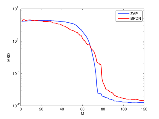
Figure 1: The reconstruction MSD versus the number of measurements $M$.

4 Experiment and Discussion

Computer simulation is presented in this section to verify the performance of the proposed algorithm compared with typical sequential CS reconstruction algorithm for solving BPDN problem [6], whose MATLAB code can be downloaded from the website [9]. In the following experiment, the entries of each row of $\bf A$ are independently generated from normal distribution. The locations of $K$ nonzero coefficients of sparse signal $\bf x$ are randomly chosen with uniform distribution $[1,N]$. The corresponding nonzero coefficients are Gaussian with mean zero and unit variance. The system parameters are $N=256$ and $K=20$. The number of measurements $M$ increases form $1$ to $120$. The parameters for BPDN are set as the recommended values by the author. The parameters for online ZAP are $\alpha=1$, $\kappa_{0}=0.02$, $\eta_{1}=0.99$, $\eta_{2}=0.8$, $T=50$, $Q=2000$. The simulation is repeated ten times, then Mean Square Derivation (MSD) between the original signal and reconstruction signal as well as the average running time calculated.

Figure 1 shows MSD curve according to $M$. As can be seen, the performance of ZAP is better than that of BPDN. When the sparse signal is recovered successfully, the number of measurements BPDN needs is larger than $80$, while the number ZAP algorithm needs is less than 80. Figure 2 demonstrates the CPU running time as $M$ increases. Again, ZAP has the better performance. The CPU time of BPDN is twice than that of ZAP for successful recovery (according to Fig.1, here $M$ is chosen as $80$ for comparison).

5 Conclusion

We have introduced in this paper a new online signal reconstruction algorithm for sequential compressive sensing. The proposed algorithm extends ZAP to sequential scenario. And in order to improve the performance, some methods, including the warm start and variable step size, are adopted. The final experiment indicates that the proposed algorithm needs less measurements and less CPU time than the reference algorithm.

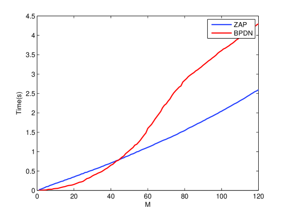
Figure 2: The CPU running time versus the number of measurements $M$.

References

- [1] D. L. Donoho, “Compressed sensing,” IEEE Trans. on Information Theory, 52(4), pp.1289-1306, April 2006.
- [2] E. Candes, J. Romberg, and T. Tao, “Robust uncertainty principles: Exact signal reconstruction from highly incomplete frequency information,” IEEE Trans. Inform. Theory, 52:489-509, 2006.
- [3] M. Lustig, D. Donoho, and J. Pauly, “Sparse MRI: The application of compressed sensing for rapid MR imaging,” Magnetic Resonance in Medicine, 58(6) pp. 1182 - 1195, December 2007.
- [4] M. Mishali, Y. C. Eldar, and J. A. Tropp, “Efficient sampling of sparse wideband analog signals,” CCIT Report #705 , October 2008.
- [5] D. Malioutov, S. Sanghavi, and A. Willsky, “Compressed sensing with sequential observations,” ICASSP, pp. 3357-3360, April 2008.
- [6] M. S. Asif and J. Romberg, “Streaming measurements in compressive sensing: filtering,” 42nd ACSSC, 26-29, Oct. 2008.
- [7] P. Garrigues and L. Ghaoui, “An homotopy algorithm for the lasso with online observations,” NISP conference, 2008.
- [8] J. Jin, Y. Gu, and S. Mei, “A stochastic gradient approach on compressive sensing signal reconstruction based on adaptive filtering framework,” IEEE Journal of Selected topics in Signal Processing, 4(2), pp.409-420, 2010.
- [9] http://users.ece.gatech.edu/sasif/homotopy/