Continuous Galerkin finite element methods for hyperbolic integro-differential equations

Abstract.

A hyperbolic integro-differential equation is considered, as a model problem, where the convolution kernel is assumed to be either smooth or no worse than weakly singular. Well-posedness of the problem is studied in the context of semigroup of linear operators, and regularity of any order is proved for smooth kernels. Energy method is used to prove optimal order a priori error estimates for the finite element spatial semidiscrete problem. A continuous space-time finite element method of order one is formulated for the problem. Stability of the discrete dual problem is proved, that is used to obtain optimal order a priori estimates via duality arguments. The theory is illustrated by an example.

1. Introduction

We consider, for any fixed $T>0$, a hyperbolic type integro-differential equation of the form

(1.1) $$\ddot{u}+Au-\int_{0}^{t}\mathcal{K}(t-s)Au(s)\,ds=f,\quad t\in(0,T),\quad{\rm with}\ u(0)=u^{0},\ \dot{u}(0)=u^{1},$$

(we use ‘$\cdot$’ to denote ‘$\frac{\partial}{\partial t}$’) where $A$ is a self-adjoint, positive definite, uniformly elliptic second order operator on a Hilbert space. The kernel $\mathcal{K}$ is considered to be either smooth (exponential), or no worse than weakly singular, and in both cases with the properties that

(1.2) $$\mathcal{K}\geq 0,\quad\dot{\mathcal{K}}(t)\leq 0,\quad\|\mathcal{K}\|_{L_{1}(\mathbb{R}^{+})}=\kappa<1.$$

This kind of problems arise e.g., in the thoery of linear and fractional order viscoelasticity. For examples and applications of this type of problems see, e.g., [13], [7], and references therein.

For our analysis, we define a function $\xi$ by

(1.3) $$\xi(t)=\kappa-\int_{0}^{t}\!\mathcal{K}(s)\,ds=\int_{t}^{\infty}\!\mathcal{K}(s)\,ds,$$

and, having (1.2), it is easy to see that

(1.4) $$\begin{split}D_{t}\xi(t)=-\mathcal{K}(t)<0,\quad\xi(0)=\kappa,\quad\lim_{t\to\infty}\xi(t)=0,\quad 0<\xi(t)\leq\kappa.\end{split}$$

Hence, $\xi$ is a completely monotone function, since

$$(-1)^{j}D_{t}^{j}\xi(t)\geq 0,\quad t\in(0,\infty),\,j=0,1,2,$$

and consequently $\xi\in L_{1,loc}[0,\infty)$ is a positive type kernel, that is, for any $T\geq 0$ and $\phi\in\mathcal{C}([0,T])$,

(1.5) $$\int_{0}^{T}\!\int_{0}^{t}\!\xi(t-s)\phi(t)\phi(s)\,ds\,dt\geq 0.$$

From the extensive literature on theoritical and numerical analysis for partial differential equations with memory, we mention [13], [7], [2], [10], [14], and their references.

The fractional order kernels, such as Mittag-Leffler type kernels in fractional viscoelasticity, interpolate between smooth (exponential) kernels and weakly singular kernels, that are singular at origin but integrable on finite time intervals $(0,T)$, for any $T\geq 0$, see [15] and references therein. This is the reason for considering problem (1.1) with convolution kernels satisfying (1.2).

In [7] well-posedness of a problem, similar to (1.1) with a Mittag-Leffler type kernel, was studied in the framework of the linear semigroup theory. Here we first extend the theory to prove higher regularity of the solution for more smooth kernels, such that a priori error estimates are fulfilled. We prove $L_{\infty}(L_{2})$ optimal order a priori error estimate, by energy methods, for finite element spatial semidiscrete approximate solution. This provides an alternative proof to what we presented in [7], and is straightforward. The continuous space-time finite element method of order one, cG(1)cG(1), is used to formulate the fully dicrete problem. A similar method has been applied to the wave equation in [5], where adaptive methods based on dual weighted residual (DWR) method has been studied. An energy identity is proved for the discrete dual problem, using the positive type auxiliary function $\xi$. This is then used to prove $L_{\infty}(L_{2})$ and $L_{\infty}(H^{1})$ optimal order a priori error estimates by duality. This and [14], where a posteriori error analysis of this method has been studied via duality, complete the error analysis of this method for model problems similar to (1.1).

The present work also extend previous works, e.g., [2], [1], [18], on quasi-static fractional order viscoelsticity $(\ddot{u}\approx 0)$ to the dynamic case. Spatial finite element approximation of integro-differential equations similar to (1.1) have been studied in [3] and [8], however, for optimal order $L_{\infty}(L_{2})$ a priori error estimate for the solution $u$, they require one extra time derivative regularity of the solution. A dynamic model for viscoelasticity based on internal variables is studied in [13]. The memory term generates a growing amount of data that has to be stored and used in each time step. This can be dealt with by introducing “sparse quadrature” in the convolution term [19]. For a different approach based on “convolution quadrature”, see [17]. However, we should note that this is not an issue for exponentially decaying memory kernels, in linear viscoelasticity, that are represented as a Prony series. In this case recurrence relationships can be derived which means recurrence formula are used for history updating, see [18] and [9] for more details. In practice, the global regularity needed for a priori error analysis is not present, e.g., due to the mixed boundary conditions, that calls for adaptive methods based on a posteriori error analysis. We plan to address these issues in future work.

In the sequel, in $\S 2$, well-posedness of the problem is proved and high regularity of the solution of the problem with smooth kernels is verified. In $\S 3$, the spatial finite element discretization is studied and, using energy method, optimal order a priori error estimates are proved. The continuous space-time finite element method of order one is applied to the problem in $\S 4$, and stability estimates for the discrete dual problem are obtained. These are then used to prove optimal order a priori error estimates in $\S 5$ by duality. Finally, in $\S 6$, we illustrate the theory by a simple example.

2. Well-posedness and regularity

We use the semigroup theory of linear operators to show that there is a unique solution of (1.1), and we prove that under appropriate assumptions on the data we get higher regularity of the solution. In $\S 2.1$ we quote the main framework from [7], to prove existence and uniqueness, to be complete. Here we restrict to pure homogeneous Dirichlet boundary condition, though the presented framework applies also to mixed homogeneous Dirichlet-Neumann boundary conditions. But it does not admit mixed homogeneuos Dirichlet nonhomogeneous Neumann boundary conditions, and this case has been studied in [15] for a more general problem, by means of Galerkin approximation method. Then in $\S 2.2$ we extend the semigroup framework to prove regularity of any order for models with smooth kernels. To this end, we specialize to the homogeneous Dirichlet boundary condition.

2.1. Existence and uniqueness

We let $\Omega\subset\mathbb{R}^{d}$, be a bounded convex domain with smooth boundary $\partial\Omega$. In order to describe the spatial regularity of functions, we recall the usual Sobolev spaces $H^{s}=H^{s}(\Omega)^{d}$ with the corresponding norms and inner products, and we denote $H=H^{0}=L_{2}(\Omega)^{d},\ V=H_{0}^{1}(\Omega)^{d}$. We equip $V$ with the energy inner product $a(u,v)=(Au,v)$ and norm $\|v\|_{V}^{2}=a(v,v)$. We recall that $A$ is a selfadjoint, positive definite, unbounded linear operator, with $\mathcal{D}(A)=H^{2}\cap V$, and we use the norms $\|v\|_{s}=\|A^{s/2}v\|$. We note that with mixed homogeneous Dirichlet-Neumann boundary conditions, we have

$$V=\{v\in H^{1}:v=0\text{\ on Dirichlet boundary}\}.$$

We extend $u$ by $u(t)=h(t)$ for $t<0$ with $h$ to be chosen. By adding $-\int_{-\infty}^{0}K(t-s)Ah(s)\,ds$ to both sides of (1.1), changing the variables in the convolution terms and defining $w(t,s)=u(t)-u(t-s)$, we get

(2.1) $$\ddot{u}(t)+(1-\kappa)Au(t)+\int_{0}^{\infty}\!\mathcal{K}(s)Aw(t,s)\,ds=f(t)-\int_{t}^{\infty}\!\mathcal{K}(s)Ah(t-s)\,ds,$$

where, we recall that $\|\mathcal{K}\|_{L_{1}(\mathbb{R}^{+})}=\kappa<1$. For latter use, we note that equation (1.1) can be retained from (2.1) by backward calculations.

For a given integer number $r\geq 0$, we use the Taylor expansion of order $r$ of the solution $u$ at $t=0$ to define the extension $u(t)=h_{r}(t)$ for $t<0$. That is, we set

(2.2) $$u(t)=h_{r}(t)=\sum_{n=0}^{r}\frac{t^{n}}{n!}u^{n}(0),\quad t<0,$$

where we use the notation $u^{n}(t)=u^{n}(t,\cdot)=\frac{\partial^{n}}{\partial t^{n}}u(t,\cdot)$, with $u^{0}(t)=u(t)$.

Now we reformulate the model problem (1.1) to an abstract Cauchy problem. First, we choose $r=0$ in (2.2), that is $h_{0}(t)=u^{0}$, and for the initial data we assume that $u^{0}\in\mathcal{D}(A)$ and $u^{1}\in V$. Therefore, from (2.1), we have

(2.3) $$\ddot{u}(t)+(1-\kappa)Au(t)+\int_{0}^{\infty}\!\mathcal{K}(s)Aw(t,s)\,ds=f(t)-Au^{0}\int_{t}^{\infty}\!\mathcal{K}(s)\ ds,$$

where,

$$w(t,s)=\left\{\begin{aligned} &u(t)-u(t-s),&&s\in[0,t],\\ &u(t)-u^{0},&&s\in[t,\infty).\end{aligned}\right.$$

Then we write (2.3), together with the initial conditions, as an abstract Cauchy problem and prove well-posedness.

We set $v=\dot{u}$ and define the Hilbert spaces

$$\begin{split}W&=L_{2,\mathcal{K}}\big{(}\mathbb{R}^{+};V\big{)}=\Big{\{}w:\lVert w\rVert_{W}^{2}=\int_{0}^{\infty}\!\mathcal{K}(s)\lVert w(s)\rVert_{V}^{2}\,ds<\infty\Big{\}},\\ Z&=V\times H\times W=\Big{\{}z=(u,v,w):\lVert z\rVert_{Z}^{2}=(1-\kappa)\lVert u\rVert_{V}^{2}+\lVert v\rVert^{2}+\lVert w\rVert_{W}^{2}<\infty\Big{\}}.\end{split}$$

We also define the linear operator $\mathcal{A}$ on $Z$ such that, for $z=(u,v,w),$

$$\mathcal{A}z=\bigg{(}v\,,\,-A\Big{(}(1-\kappa)u+\int_{0}^{\infty}\!\mathcal{K}(s)w(s)\,ds\Big{)}\,,\,v-Dw\bigg{)},$$

with domain of definition

$$\mathcal{D}(\mathcal{A})=\Big{\{}(u,v,w)\in Z:v\in V,\,(1-\kappa)u+\int_{0}^{\infty}\!\mathcal{K}(s)w(s)\,ds\in\mathcal{D}(A),w\in\mathcal{D}(D)\Big{\}}.$$

Here $Dw=\frac{d}{ds}w$ with $\mathcal{D}(D)=\{w\in W:Dw\in W\,\,{\rm and}\,\,w(0)=0\}.$

Therefore, a solution of (1.1) satisfies the system of delay differential equations, for $t\in(0,T)$,

$$\begin{split}\dot{u}(t)&=v,\\ \dot{v}(t)&=-A\Big{(}(1-\kappa)u(t)+\int_{0}^{\infty}\!\mathcal{K}(s)w(t,s)\,ds\Big{)}+f(t)-Au^{0}\int_{t}^{\infty}\!\mathcal{K}(s)\ ds,\\ \dot{w}(t,s)&=v(t)-Dw(t,s),\quad s\in(0,\infty).\end{split}$$

This can be writen as the abstract Cauchy problem

(2.4) $$\begin{split}&\dot{z}(t)=\mathcal{A}z(t)+F(t),\quad t\in(0,T),\\ &z(0)=z^{0},\end{split}$$

where $F(t)=(0,f(t)-Au^{0}\int_{t}^{\infty}\!\mathcal{K}(s)\ ds,0)$ and $z^{0}=\big{(}u^{0},u^{1},0\big{)}$, since

$$w(0,s)=u(0)-u(-s)=u(0)-h(-s)=u^{0}-u^{0}=0.$$

We note that $w(t,0)=u(t)-u(t)=0$, so that $w(t,\cdot)\in\mathcal{D}(D)$.

We quote from [7, Theorem 2.2], that $\mathcal{A}$ generates a $C_{0}$-semigroup of cotractions on $Z$.

Corollary 1.

The linear operator $\mathcal{A}$ is an infinitesimal generator of a $C_{0}$-semigroup $e^{t\mathcal{A}}$ of contractions on the Hilbert space $Z$.

Now, we look for a strong solution of the initial value problem (2.4), that is, a function $z$ which is differentiable a.e. on $[0,T]$ with $\dot{z}\in L_{1}((0,T);Z)$, if $z(0)=z^{0}$, $z(t)\in\mathcal{D}(\mathcal{A})$, and $\dot{z}(t)=\mathcal{A}z(t)+F(t)$ a.e. on $[0,T]$.

Recalling the assumptions $u^{0}\in\mathcal{D}(A)$ and $u^{1}\in V$, we know that if $z=(u,v,w)$ be a strong solution of the abstract Cauchy problem (2.4) with $z^{0}=\big{(}u^{0},u^{1},0\big{)}$, then $u$ is a solution of (1.1) by [7, Lemma 2.1]. Hence, to prove that there is a unique solution for (1.1), we need to prove that there is a unique strong solution for (2.4). This has been proved in [7, Theorem 2.2], if $f:[0,T]\to H$ is Lipschitz continuous, using the fact that the linear operator $\mathcal{A}$ generates a $C_{0}$-semigroup of contractions on $Z$. Moreover, for some $C=C(\kappa,T)$, we have the regularity estimate, for $t\in[0,T]$,

(2.5) $$\lVert u(t)\rVert_{V}+\lVert\dot{u}(t)\rVert\leq C\Big{(}\lVert Au^{0}\rVert+\lVert u^{1}\rVert+\int_{0}^{t}\!\lVert f\rVert\,ds\Big{)}.$$

2.2. High order regularity

In order to prove higher regularity of order $r+1$ ($\ r\geq 1$), we assume that the bounded domain $\Omega$ is convex, and we specialize to the homogeneous Dirichlet boundary condition. Hence, the elliptic regularity estimate holds, that is

(2.6) $$\|u\|_{2}\leq C\|Au\|,\quad u\in\mathcal{D}(A)=H^{2}\cap V.$$

We note that the case $r=0$ is the choice for (2.5). We substitute $h_{r}(t)$ from (2.2), with $r\geq 1$, in (2.1). Then, differentiating $\frac{\partial^{r}}{\partial t^{r}}$ and using the notation $u^{r}(t)=\frac{\partial^{r}}{\partial t^{r}}u(t)$, we have

(2.7) $$\begin{split}\ddot{u}^{r}(t)&+(1-\kappa)Au^{r}(t)+\int_{0}^{\infty}\!\!\mathcal{K}(s)Aw^{r}(t,s)\,ds\\ &\qquad=f^{r}(t)-A\frac{\partial^{r}}{\partial t^{r}}\int_{t}^{\infty}\!\mathcal{K}(s)\sum_{n=0}^{r}\frac{(t-s)^{n}}{n!}u^{n}(0)\ ds\\ &\qquad=f^{r}(t)+A\sum_{n=0}^{r-1}u^{n}(0)\mathcal{K}^{r-n-1}(t)-Au^{r}(0)\xi(t)\\ &\qquad=:\tilde{f}^{r}(t),\end{split}$$

with the initial data $u^{r}(0),u^{r+1}(0)$.

Recalling the initial data $u(0)=u^{0}$ and $u^{1}(0)=u^{1}$, from (1.1), we have $u^{2}(0)=f(0)-Au^{0}$. To obtain $u^{m}(0),\ m\geq 3$, we differentiate $\frac{\partial^{m-2}}{\partial t^{m-2}}$ of equation (1.1), and we have

(2.8) $$\ddot{u}^{m-2}(t)+Au^{m-2}(t) -\int_{0}^{t}\mathcal{K}^{m-2}(t-s)Au(s)\,ds$$

$$=f^{m-2}(t)+A\sum_{n=0}^{m-3}u^{n}(t)\mathcal{K}^{m-n-3}(0),\quad t\in(0,T),$$

that, with $t=0$, implies the initial condition

(2.9) $$u^{m}(0)=f^{m-2}(0)-Au^{m-2}(0)+\sum_{n=0}^{m-3}Au^{n}(0)\mathcal{K}^{m-n-3}(0), m\geq 3.$$

Throughout, obviously any sum $\sum_{n=i}^{j}$ is supposed to be suppressed from the formulas, when $i>j$.

Remark 1.

We note that, if we assume $\mathcal{K}\in W_{1}^{m-2}(0,T)$, then $\mathcal{K}\in\mathcal{C}^{m-3}[0,T]$ by Sobolev inequality, and therefore $u^{m}(0)$ is well-defined.

Remark 2.

One can show, by induction and the fact that by (2.6)

(2.10) $$\|v\|\leq\|v\|_{H^{2}}\leq C\|Av\|,\quad\text{for}\ v\in\mathcal{D}(A),$$

we have $(m=0,1,\ k=1,2,\cdots)$,

(2.11) $$\begin{split}|A^{m}u^{2k}(0)|&\leq C\Big{(}|A^{m+k}u^{0}|+|A^{m+k-1}u^{1}|\\ &\quad+\sum_{j=0}^{k-1}|A^{m+j}f^{2k-2j-2}(0)|+\sum_{j=1}^{k-2}|A^{m+j}f^{2k-2j-3}(0)|\Big{)},\end{split}$$

(2.12) $$\begin{split}|A^{m}u^{2k+1}(0)|&\leq C\Big{(}|A^{m+k}u^{0}|+|A^{m+k}u^{1}|\\ &\quad+\sum_{j=1}^{k-1}|A^{m+j}f^{2k-2j-2}(0)|+\sum_{j=0}^{k-1}|A^{m+j}f^{2k-2j-1}(0)|\Big{)}.\end{split}$$

Now we note that, in (2.7), we have

$$w^{r}(t,s)=\left\{\begin{aligned} &u^{r}(t)-u^{r}(t-s),&&s\in[0,t],\\ &u^{r}(t)-u^{r}(0),&&s\in[t,\infty),\end{aligned}\right.$$

so that $w^{r}(t,0)=0$. Therefore, considering continuty of $w^{r}$, we have $w^{r}\in\mathcal{D}(D)$.

Then, in the same way as in the previous section, with $v^{r}=\dot{u}^{r}$, we can reformulate (2.7), with $z^{r}=(u^{r},v^{r},w^{r})$, as the abstract Cauchy problem

(2.13) $$\begin{split}&\dot{z}^{r}(t)=\mathcal{A}\,z^{r}(t)+F^{r}(t),\quad 0<t<T,\\ &z^{r}(0)=z^{r,0},\end{split}$$

where $F^{r}(t)=(0,\tilde{f}^{r}(t),0)$ and $z^{r,0}=(u^{r}(0),u^{r+1}(0),0)$, since $w^{r}(0,s)=u^{r}(0)-u^{r}(0)=0$.

In particular, for $r=1$, we have

$$F^{1}(t)=\Big{(}0,f^{1}(t)+Au^{0}\mathcal{K}(t)-Au^{1}\xi(t),0\Big{)},$$

with initial data $z^{1,0}=(u^{1},u^{2}(0),0)=(u^{1},f(0)-Au^{0},0)$.

Now, we need to show that from a strong solution of the abstract Cauchy problem (2.13), for $r\geq 1$, we get a solution of the main problem (1.1). Therfore we should prove that the abstract Cauchy problem (2.13) has a unique strong solution, under certain conditions on the data. The proof is by induction, and therefore we recall some facts from [7], for $r=1$.

Lemma 1.

Let $z^{1}=(u^{1},v^{1},w^{1})$ be a strong solution of the abstract Cauchy problem (2.13) with $z^{1,0}=\big{(}u^{1},u^{2}(0),0\big{)}$. Then $u(t)=u^{0}+\int_{0}^{t}u^{1}(s)\,ds$ is a solution of (1.1).

Theorem 1.

There is a unique solution $u=u(t)$ of (1.1) if $\mathcal{K}\in W_{1}^{1}(\mathbb{R}^{+})$ with $\|\mathcal{K}\|_{W_{1}^{1}(\mathbb{R}^{+})}<1$, $f(0)-Au^{0}\in V,\ u^{1}\in\mathcal{D}(A)$, and $\dot{f}:[0,T]\to H$ is Lipschitz continuous. Moreover, for some $C=C(\kappa,T)$, we have the regularity estimate, for $t\in[0,T]$,

(2.14) $$\lVert\dot{u}(t)\rVert_{V}+\lVert\ddot{u}(t)\rVert\leq C\Big{(}\lVert Au^{0}\rVert+\lVert Au^{1}\rVert+\lVert f(0)\rVert+\int_{0}^{t}\!\lVert\dot{f}\rVert\,ds\Big{)}.$$

Proof.

There exists a unique strong solution $z^{1}=(u^{1},v^{1},w^{1})$ for (2.13), with $r=1$, by [7, Theorem 2.4]. Hence, the proof is complete by Lemma 1. ∎

Lemma 2.

Let $z^{r}=(u^{r},v^{r},w^{r})$, for $r\geq 1$, be a strong solution of the abstract Cauchy problem (2.13) with $z^{r,0}=(u^{r}(0),u^{r+1}(0),0)$. Then $u(t)=u^{0}+\int_{0}^{t}u^{1}(s)\,ds$ is a solution of (1.1).

Proof.

The proof is by induction. The case $r=1$ follows from Theorem 1.

Now, we assume that the lemma valids for some $r\geq 2$, and we prove that it holds also for $r+1$. To this end, we show that if $z^{r+1}=(u^{r+1},v^{r+1},w^{r+1})$ be a strong solution of (2.13) (for $r+1$) with $z^{r+1,0}=(u^{r+1}(0),u^{r+2}(0),0)$, then $z^{r}=(u^{r},v^{r},w^{r})$ is a strong solution of (2.13) with $z^{r,0}=(u^{r}(0),u^{r+1}(0),0)$, that completes the proof by induction assumption.

Since $\dot{z}^{r+1}(t)=\mathcal{A}\,z^{r+1}(t)+F^{r+1}(t)$ a.e. on $[0,T]$, we have, for $t\in(0,T)$,

$$\begin{split}&\dot{u}^{r+1}(t)=v^{r+1}(t),\\ &\dot{v}^{r+1}(t)=-A\Big{(}(1-\kappa)u^{r+1}(t)+\int_{0}^{\infty}\!\mathcal{K}(s)w^{r+1}(t,s)\,ds\Big{)}+\tilde{f}^{r+1}(t),\\ &\dot{w}^{r+1}(t,s)=v^{r+1}(t)-Dw^{r+1}(t,s),\ s\in(0,\infty).\end{split}$$

The first and the third equation implies that $w^{r+1}$ satisfies the first order partial differential equation

$$w^{r+1}_{t}+w^{r+1}_{s}=u^{r+1}_{t}.$$

This, with $w^{r+1}(t,0)=0,\,w^{r+1}(0,s)=0$, has the unique solution $w^{r+1}(t,s)=u^{r+1}(t)-u^{r+1}(t-s)$, that implies, by integration with respect to $t$,

$$w^{r}(t,s)=u^{r}(t)-u^{r}(t-s)=\int_{0}^{t}\!w^{r+1}(\tau,s)\,d\tau.$$

From the first and the second equations we obtain equation (2.7) with $r+1$, that is obtained from equation (2.1) by differentiating $\frac{\partial^{r}}{\partial t^{r}}$. We recall that equations (1.1) and (2.1) are equivalent, that implies equivalence of equations (2.7) and (2.8). Therefore $u$ also satisfies (2.8) with $r+1$. Then, integrating with respect to $t$, we have, for $t\in(0,T)$,

(2.15) $$\ddot{u}^{r}(t)-\ddot{u}^{r} (0)+Au^{r}(t)-Au^{r}(0)-\int_{0}^{t}\int_{0}^{\tau}\!\mathcal{K}^{r+1}(\tau-s)Au(s)\ ds\ d\tau$$

$$=f^{r}(t)-f^{r}(0)+A\sum_{n=0}^{r}\int_{0}^{t}\!u^{n}(\tau)\ d\tau\mathcal{K}^{r-n}(0).$$

Now, we need to show that (2.15) implies (2.8). We note that

$$\int_{0}^{t}\int_{0}^{\tau}\!\mathcal{K}^{r+1}(\tau-s)Au(s)\ ds\ d\tau =\int_{0}^{t}\int_{s}^{t}\!\mathcal{K}^{r+1}(\tau-s)Au(s)\ d\tau\ ds$$

$$=\int_{0}^{t}\!\mathcal{K}^{r}(t-s)Au(s)\ ds-A\mathcal{K}^{r}(0)\int_{0}^{t}\!u(s)\ ds,$$

and

$$A\sum_{n=0}^{r} \int_{0}^{t}\!u^{n}(\tau)\ d\tau\mathcal{K}^{r-n}(0)$$

$$=A\bigg{(}\int_{0}^{t}\!u(\tau)\ d\tau\mathcal{K}^{r}(0)+\sum_{n=1}^{r}\big{(}u^{n-1}(t)-u^{n-1}(0)\big{)}\mathcal{K}^{r-n}(0)\bigg{)}$$

$$=A\mathcal{K}^{r}(0)\int_{0}^{t}\!u(\tau)\ d\tau+A\sum_{n=0}^{r-1}u^{n}(t)\mathcal{K}^{r-n-1}(0)-A\sum_{n=0}^{r-1}u^{n}(0)\mathcal{K}^{r-n-1}(0).$$

Using these and (2.9) in (2.15) we conclude (2.8), that is equivalent to (2.7). This means that, $z^{r}=(u^{r},v^{r},w^{r})$ is a strong solution of (2.13) with $z^{r,0}=(u^{r}(0),u^{r+1}(0),0)$. Hence, by induction assumption, $u(t)=u^{0}+\int_{0}^{t}u^{1}(s)\,ds$ is a solution of (1.1), and this completes the proof. ∎

In the next theorem we find the circumstances under which there is a unique strong solution of the abstract Cauchy problem (2.13), that by Lemma 2 implies existence of a unique solution of (1.1) with higher regularity. We also obtain regularity estimates, which are extensions of (2.5) and (2.14).

We note that, recalling Remark 1 and having the assumptions from the next theorem, the calculations in the proof of Lemma 2 make sense.

Theorem 2.

For a given integer number $r\geq 1$, let $f^{r}=\frac{\partial^{r}}{\partial t^{r}}f:[0,T]\to H$ be Lipschitz continuous and $\mathcal{K}\in W^{r}_{1}(\mathbb{R}^{+})$ with $\|\mathcal{K}\|_{W^{r}_{1}(\mathbb{R}^{+})}<1$. We also, recalling $\mathcal{D}(A)=H^{2}\cap V$, assume the following compatibility conditions:

for $r=2k\,(k=1,2,\cdots)$,

(2.16) $$\begin{split}&A^{k}u^{0}\in\mathcal{D}(A),\quad A^{k}u^{1}\in V,\\ &f^{r-2j}(0)\in H^{2j}\cap V,\quad j=1,\cdots,\,k,\ k\geq 1,\\ &f^{r-2j+1}(0)\in H^{2(j-1)}\cap V,\quad j=1,\cdots,\,k,\ k\geq 1,\end{split}$$

and for $r=2k+1\,(k=0,1,2,\cdots)$,

(2.17) $$\begin{split}&A^{k}u^{1}\in\mathcal{D}(A),\quad A^{k+1}u^{0}\in V,\\ &f^{r-2j}(0)\in H^{2j}\cap V,\quad j=1,\cdots,k,\ k\geq 1,\\ &f^{r-2j+1}(0)\in H^{2(j-1)}\cap V,\quad j=1,\cdots,k+1,\ k\geq 0.\end{split}$$

Then there is a unique solution of (1.1).

Moreover, for some $C=C(\kappa,\|\mathcal{K}\|_{W^{r}_{1}(\mathbb{R}^{+})},T)$:

for $r=2k\,(k=1,2,\cdots)$, we have the regularity estimate

(2.18) $$\begin{split}\lVert u^{r}(t)\rVert_{V}&+\lVert u^{r+1}(t)\rVert\\ &\leq C\bigg{(}\lVert A^{k+1}u^{0}\rVert+\lVert A^{k}u^{1}\rVert\\ &\quad+\sum_{j=1}^{k}\lVert A^{j}f^{r-2j}(0)\rVert+\sum_{j=1}^{k}\lVert A^{j-1}f^{r-2j+1}(0)\rVert+\int_{0}^{t}\!\lVert f^{r}(s)\rVert\,ds\bigg{)},\end{split}$$

and, for $r=2k+1\,(k=0,1,2,\cdots)$, we have the estimate

(2.19) $$\begin{split}\lVert u^{r}(t)\rVert_{V}&+\lVert u^{r+1}(t)\rVert\\ &\!\!\!\!\!\leq C\bigg{(}\lVert A^{k+1}u^{0}\rVert+\lVert A^{k+1}u^{1}\rVert\\ &+\sum_{j=1}^{k}\lVert A^{j}f^{r-2j}(0)\rVert+\sum_{j=1}^{k+1}\lVert A^{j-1}f^{r-2j+1}(0)\rVert+\int_{0}^{t}\!\lVert f^{r}(s)\rVert\,ds\bigg{)}.\end{split}$$

Proof.

1. The case $r=1$ follows from Theorem 1. Then, for a given $r\geq 2$, we show that

• $z^{r}(0)=z^{r,0}=(u^{r}(0),u^{r+1}(0),0)\in\mathcal{D}(\mathcal{A})$,

• $F^{r}$ is differentiable almost everywhere on $[0,T]$ and $\dot{F}\in L_{1}([0,T];Z)$.

These imply existence of a unique strong solution of the abstract Cauchy problem (2.13), by [11, Corollary 4.2.10], that yields existence of a unique solusion of (1.1), by Lemma 2.

2. First we note that (i) holds, if $u^{r}(0)\in\mathcal{D}(A)$ and $u^{r+1}(0)\in V$, by the definition of $\mathcal{D}(\mathcal{A})$. This can be verified by applying the compatibility conditions (2.16)–(2.17) in (2.11)–(2.12), using (2.10).

3. Now we prove (ii). By assumption $f^{r}:[0,T]\to H$ is Lipschitz continuous. Therefore, by a classical result from functional analysis, $f^{r}$ is differentiable almost everywhere on $[0,T]$ and $\dot{f}^{r}\in L_{1}([0,T];H)$, since $H$ is a Hilbert space. Then, recalling the assumption $\mathcal{K}\in W_{1}^{r}(\mathbb{R}^{+})$ and the fact that

$$\dot{\tilde{f}}^{r}(t)=\dot{f}^{r}(t)+A\sum_{n=0}^{r}u^{n}(0)\mathcal{K}^{r-n}(t),$$

we conclude that $F^{r}(t)=(0,\tilde{f}^{r}(t),0)$ is differentiable almost everywhere on $[0,T]$ and $\dot{F}^{r}\in L_{1}([0,T];Z)$, that completes the proof of (ii).

4. Hence, since $\mathcal{A}$ generates a $C_{0}$-semigroup of contractions on $Z$ by Corollary 1, we conclude, by [11, Corollary 4.2.10], that there exists a unique strong solution $z^{r}=(u^{r},v^{r},w^{r})$ for the abstract Cauchy problem (2.13). This, by Lemma 2, proves that there is a unique solution $u$ of (1.1), that completes the first part of the theorem.

5. Finally, we prove the regularity estimates (2.18) and (2.19) for $r\geq 2$, since the case $r=1$ follows from Theorem 1.

The unique strong solution $z^{r}=(u^{r},v^{r},w^{r})$ of (2.13), is given by

$$z^{r}(t)=e^{t\mathcal{A}}z^{r,0}+\int_{0}^{t}\!e^{(t-s)\mathcal{A}}F^{r}(s)\,ds,$$

and we recall the fact that $\lVert e^{t\mathcal{A}}\rVert_{Z}\leq 1$, since $\mathcal{A}$ is an infinitesimal generator of a $C_{0}$ semigroup of contractions on $Z$. Therefore

$$\lVert z^{r}(t)\rVert_{Z}\leq\lVert z^{r,0}\rVert_{Z}+\int_{0}^{t}\!\lVert F^{r}(s)\rVert_{Z}\,ds.$$

Since $v^{r}=\dot{u}^{r}=u^{r+1}$, $z^{r,0}=(u^{r}(0),u^{r+1}(0),0)$, and

$$\begin{split}\lVert F^{r}(s)\rVert_{Z}=\lVert\tilde{f^{r}}(s)\rVert&=\lVert f^{r}(s)\|+\sum_{n=0}^{r-1}\|Au^{n}(0)\||\mathcal{K}^{r-n-1}(s)|+\|Au^{r}(0)\||\xi(s)|,\end{split}$$

therefore we have

$$\begin{split}\Big{(}(1-\kappa)\lVert u^{r}(t)\rVert_{V}^{2}&+\lVert u^{r+1}(t)\rVert^{2}\Big{)}^{1/2}\\ &\leq\big{(}(1-\kappa)\lVert u^{r}(0)\rVert_{V}^{2}+\lVert u^{r+1}(0)\rVert^{2}\big{)}^{1/2}\\ &\quad+\int_{0}^{t}\!\rVert f^{r}(s)\rVert\ ds+\sum_{n=0}^{r-1}\|Au^{n}(0)\|\int_{0}^{t}\!|\mathcal{K}^{r-n-1}(s)|\ ds\\ &\quad+\|Au^{r}(0)\|\int_{0}^{t}\!|\xi(s)|\ ds.\end{split}$$

Hence, considering the assumption that $\|\mathcal{K}\|_{W_{1}^{r}(\mathbb{R}^{+})}<1$, we have, for some $C=C(\kappa,\|\mathcal{K}\|_{W_{1}^{r}(\mathbb{R}^{+})},T)$,

(2.20) $$\begin{split}\lVert u^{r}(t)\rVert_{V}+\lVert u^{r+1}(t)\rVert&\leq C\bigg{(}\lVert u^{r}(0)\rVert_{V}+\lVert u^{r+1}(0)\rVert\\ &\quad+\int_{0}^{t}\!\rVert f^{r}(s)\rVert\ ds+\sum_{n=0}^{r}\|Au^{n}(0)\|\bigg{)}.\end{split}$$

Since, by elliptic regularity estimate (2.6),

$$\|u^{r}(0)\|_{V}\leq\|u^{r}(0)\|_{H^{2}}\leq C\|Au^{r}(0)\|,$$

so we have

$$\begin{split}\lVert u^{r}(t)\rVert_{V}+\lVert u^{r+1}(t)\rVert&\leq C\bigg{(}\|u^{r+1}(0)\|+\sum_{n=0}^{r}\|Au^{n}(0)\|+\int_{0}^{t}\!\rVert f^{r}(s)\rVert\ ds\bigg{)},\end{split}$$

that, by (2.10)–(2.12), implies the regularity estimates (2.18)–(2.19). Now, the proof is complete. ∎

3. The spatial finite elment discretization

The variational form of (1.1) is to find $u(t)\in V$, such that $u(0)=u^{0}$, $\dot{u}(0)=u^{1}$, and for $t\in(0,T)$,

(3.1) $$(\ddot{u},v)+a(u,v)-\int_{0}^{t}\!\mathcal{K}(t-s)a(u(s),v)\ ds=(f,v),\quad\forall v\in V.$$

Let $\Omega$ be a convex polygonal domain and $\{\mathcal{T}_{h}\}$ be a regular family of triangulations of $\Omega$ with corresponding family of finite element spaces $V_{h}^{l}\subset V$, consisting of continuous piecewise polynomials of degree at most $l-1$, that vanish on $\partial\Omega$ (so the mesh is required to fit $\partial\Omega$). Here $l\geq 2$ is an integer number. We define piecewise constant mesh function $h_{K}(x)=\textrm{diam}(K)$ for $x\in K,\,K\in\mathcal{T}_{h}$, and for our error analysis we denote $h=\max_{K\in\mathcal{T}_{h}}h_{K}$. We note that the finite element spaces $V_{h}^{l}$ have the property that

(3.2) $$\min_{\chi\in V_{h}^{l}}\{\|v-\chi\|+h\|v-\chi\|_{1}\}\leq Ch^{i}\|v\|_{i},\quad\textrm{for}\ v\in H^{i}\cap V,\ 1\leq i\leq l.$$

We recall the $L_{2}$-projection $\mathcal{P}_{h}:H\to V_{h}^{l}$ and the Ritz projection $\mathcal{R}_{h}:V\to V_{h}^{l}$ defined by

$$a(\mathcal{R}_{h}v,\chi)=a(v,\chi)\quad{\rm and}\quad(\mathcal{P}_{h}v,\chi)=(v,\chi),\qquad\forall\chi\in V_{h}^{l}.$$

We also recall the elliptic regularity estimate (2.6), such that the error estimates (3.2) hold true for the Ritz projection $\mathcal{R}_{h}$, see [20], i.e.,

(3.3) $$\begin{split}\|(\mathcal{R}_{h}-I)v\|+h\|(&\mathcal{R}_{h}-I)v\|_{1}\leq Ch^{i}\|v\|_{i},\quad\textrm{for}\ v\in H^{i}\cap V,\ 1\leq i\leq l.\end{split}$$

Then, the spatial finite element discretization of (3.1) is to find $u_{h}(t)\in V_{h}^{l}$ such that $u_{h}(\cdot,0)=u_{h}^{0},\ \dot{u}_{h}(\cdot,0)=u_{h}^{1}$, and for $t\in(0,T)$,

(3.4) $$(\ddot{u}_{h},v_{h})+a(u_{h},v_{h})-\int_{0}^{t}\!\mathcal{K}(t-s)a(u_{h}(s),v_{h})\ ds=(f,v_{h}),\quad\forall v_{h}\in V_{h}^{l},$$

where $u_{h}^{0}$ and $u_{h}^{1}$ are suitable approximations to be chosen, respectively, for $u_{0}$ and $u^{1}$ in $V_{h}^{l}$.

Theorem 3.

Assume that $\Omega$ is a convex polygonal domain. Let $u$ and $u_{h}$ be, respectively, the solutions of (3.1) and (3.4). Then

(3.5) $$\begin{split}\|u_{h}(T)-u(T)\|&\leq C\|u_{h}^{0}-\mathcal{R}_{h}u^{0}\|+Ch^{l}\Big{(}\|u(T)\|_{l}+\int_{0}^{T}\!\|\dot{u}\|_{l}\,d\tau\Big{)},\end{split}$$

where we assume the initial condition $u_{h}^{1}=\mathcal{P}_{h}u^{1}$.

Proof.

The proof is adapted from [4]. We split the error as

(3.6) $$e=u_{h}-u=(u_{h}-R_{h}u)+(R_{h}u-u)=\theta+\omega.$$

We need to estimate $\theta$, since the spatial projection error $\omega$ is estimated from (3.3).

So, putting $\theta$ in (3.4) we have, for $v_{h}\in V_{h}^{l}$,

$$\begin{split}(\ddot{\theta},v_{h}&)+a(\theta,v_{h})-\int_{0}^{t}\mathcal{K}(t-s)a(\theta(s),v_{h})ds\\ &=(\ddot{u}_{h},v_{h})+a(u_{h},v_{h})-\int_{0}^{t}\mathcal{K}(t-s)a(u_{h}(s),v_{h})ds\\ &\quad-(R_{h}\ddot{u},v_{h})-a(R_{h}u,v_{h})+\int_{0}^{t}\mathcal{K}(t-s)a(R_{h}u(s),v_{h})ds,\end{split}$$

that, using (3.4), the definition of the Ritz projection $\mathcal{R}_{h}$, and (3.1), we have

(3.7) $$\begin{split}(\ddot{\theta},v_{h}&)+a(\theta,v_{h})-\int_{0}^{t}\mathcal{K}(t-s)a(\theta(s),v_{h})ds\\ &=(f,v_{h})-(R_{h}\ddot{u},v_{h})-a(u,v_{h})+\int_{0}^{t}\mathcal{K}(t-s)a(u(s),v_{h})ds\\ &=(\ddot{u},v_{h})-(R_{h}\ddot{u},v_{h})=-(\ddot{\omega},v_{h}).\end{split}$$

Therefore we can write, for $v_{h}(t)\in V_{h}^{l}$, $t\in(0,T]$,

$$\frac{d}{dt}(\dot{\theta},v_{h})-(\dot{\theta},\dot{v}_{h})+a(\theta,v_{h})-\int_{0}^{t}\mathcal{K}(t-s)a(\theta(s),v_{h}(t))ds=-\frac{d}{dt}(\dot{\omega},v_{h})+(\dot{\omega},\dot{v_{h}}),$$

that, recalling $e=\theta+\omega$, we obtain

(3.8) $$-(\dot{\theta},\dot{v}_{h})+a(\theta,v_{h})-\int_{0}^{t}\mathcal{K}(t-s)a(\theta(s),v_{h}(t))ds=-\frac{d}{dt}(\dot{e},v_{h})+(\dot{\omega},\dot{v}_{h})$$

Now let $0<\varepsilon\leq T$ , and we make the particular choice

$$v_{h}(\cdot,t)=\int_{t}^{\varepsilon}\theta(\cdot,\tau)d\tau,\qquad 0\leq t\leq T,$$

then clearly we have

(3.9) $$v_{h}(\cdot,\varepsilon)=0,\quad\frac{d}{dt}v_{h}(\cdot,t)=-\theta(\cdot,t),\quad 0\leq t\leq T.$$

Hence, considering (3.9) in (3.8) , we have

$$\frac{1}{2}\frac{d}{dt}(\|\theta\|^{2}-\|v_{h}\|_{V}^{2})-\int_{0}^{t}\mathcal{K}(t-s)a(\theta(s),v_{h}(t))ds=-\frac{d}{dt}(\dot{e},v_{h})-(\dot{\omega},\theta).$$

Now, integrating from $t=0$ to $t=\varepsilon$, we have

$$\begin{split}\|\theta(\varepsilon)\|^{2}-\|\theta(0)&\|^{2}-\|v_{h}(\varepsilon)\|^{2}_{V}+\|v_{h}(0)\|^{2}_{V}-2\int_{0}^{\varepsilon}\int_{0}^{t}\mathcal{K}(t-s)a(\theta(s),v_{h}(t))dsdt\\ &=-2(\dot{e}(\varepsilon),v_{h}(\varepsilon))+2(\dot{e}(0),v_{h}(0))-2\int_{0}^{\varepsilon}(\dot{\omega},\theta)dt.\end{split}$$

Then, using the initial assuption $u_{h}^{1}=\mathcal{P}_{h}u^{1}$ that implies the second term on the right side is zero and recalling $v_{h}(\varepsilon)=0$, we conclude

(3.10) $$\begin{split}\|\theta(\varepsilon)\|^{2}+\|&v_{h}(0)\|_{V}^{2}-2\int_{0}^{\varepsilon}\int_{0}^{t}\mathcal{K}(t-s)a(\theta(s),v_{h}(t))dsdt\\ &\leq\|\theta(0)\|^{2}+2\max_{0\leq t\leq\varepsilon}\|\theta(t)\|\int_{0}^{\varepsilon}\|\dot{\omega}\|dt.\end{split}$$

Now, by changing the order of integrals, using $\frac{d}{dt}\xi(t-s)=-\mathcal{K}(t-s)$ from (1.4), and integration by parts, we can write the third term on the left side as

$$\begin{split}-2\int_{0}^{\varepsilon}\int_{0}^{t}&\mathcal{K}(t-s)a(\theta(s),v_{h}(t))dsdt=2\int_{0}^{\varepsilon}\int_{s}^{\varepsilon}\frac{d}{dt}\xi(t-s)a(\theta(s),v_{h}(t))dtds\\ &=2\int_{0}^{\varepsilon}\xi(\varepsilon-s)a(\theta(s),v_{h}(\varepsilon))ds-2\int_{0}^{\varepsilon}\xi(0)a(\theta(s),v_{h}(s))ds\\ &\qquad-2\int_{0}^{\varepsilon}\int_{s}^{\varepsilon}\xi(t-s)a(\theta(s),\dot{v}_{h}(t))dtds.\end{split}$$

Then, using (3.9) and $\xi(0)=\kappa$, we have

$$\begin{split}-2\int_{0}^{\varepsilon}&\int_{0}^{t}\mathcal{K}(t-s)a(\theta(s),v_{h}(t))dsdt\\ &=\kappa(\|v_{h}(\varepsilon)\|^{2}_{V}-\|v_{h}(0)\|^{2}_{V})+2\int_{0}^{\varepsilon}\int_{s}^{\varepsilon}\xi(t-s)a(\theta(s),\theta(t))dtds.\end{split}$$

Therefore, using this and $v_{h}(\varepsilon)=0$ in (3.10) we have

$$\begin{split}\|\theta(\varepsilon)\|^{2}+(1-\kappa)\|&v_{h}(0)\|_{V}^{2}+2\int_{0}^{\varepsilon}\int_{s}^{\varepsilon}\xi(t-s)a(\theta(s),\theta(t))dtds\\ &\leq\|\theta(0)\|^{2}+2\max_{0\leq t\leq\varepsilon}\|\theta(t)\|\int_{0}^{\varepsilon}\|\dot{\omega}\|dt,\end{split}$$

that considering the fact that $\xi$ is a positive type kernel and $\kappa<1$, in a standard way, implies that

$$\|\theta(T)\|\leq C(\|\theta(0)\|+\int_{0}^{T}\|\dot{\omega}\|d\tau).$$

Hence, recaling (3.6), we have

$$\begin{split}\|e(T)\|&\leq\|\theta(T)\|+\|\omega(T)\|\\ &\leq C\Big{(}\|u_{h}^{0}-R_{h}u^{0}\|+\int_{0}^{T}\|\dot{u}-R_{h}\dot{u}\|dt\Big{)}+\|(R_{h}u-u)(T)\|,\end{split}$$

that using the error estimate (3.3) implies the a priori error estimate (3.5). ∎

4. The continuous Galerkin method

Here we formulate a continuous space-time Galerkin finite element method of order one, cG(1)cG(1), for the primar and dual problems (4.4) and (4.8), that is based on a similar method for the wave equation in [5]. Then we prove stability estimaes for the discrete dual problem. These are then used in a priori error analysis, that is via duality.

4.1. Weak formulation

First we write a “velocity-displacement” formulation of (1.1) which is obtained by introducing a new velocity variable. We use the new variables $u_{1}=u$, $u_{2}=\dot{u}$, and $u=(u_{1},u_{2})$, then the variational form is to find $u_{1}(t),\,u_{2}(t)\in V$ such that $u_{1}(0)=u^{0}$, $u_{2}(0)=v^{0}$, and for $t\in(0,T)$,

(4.1) $$\begin{split}&(\dot{u}_{1}(t),v_{1})-(u_{2}(t),v_{1})=0,\\ &(\dot{u}_{2}(t),v_{2})+a(u_{1}(t),v_{2})-\int_{0}^{t}\mathcal{K}(t-s)a(u_{1}(s),v_{2})\,ds\\ &\qquad\qquad\qquad\quad\quad=(f(t),v_{2}),\quad\forall v_{1},v_{2}\in V.\end{split}$$

Now we define the bilinear and linear forms $B:\mathcal{U}\times\mathcal{V}\to\mathbb{R}$ and $L:\mathcal{V}\to\mathbb{R}$ by

(4.2) $$\begin{aligned} B(u,v)&=\int_{0}^{T}\!\Big{\{}(\dot{u}_{1},v_{1})-(u_{2},v_{1})+(\dot{u}_{2},v_{2})+a(u_{1},v_{2})\\ &\quad\quad-\int_{0}^{t}\!\mathcal{K}(t-s)a\big{(}u_{1}(s),v_{2}\big{)}\,ds\Big{\}}\,dt\\ &\quad+\big{(}u_{1}(0),v_{1}(0)\big{)}+\big{(}u_{2}(0),v_{2}(0)\big{)},\\ L(v)&=\int_{0}^{T}\!(f,v_{2})\,dt+\big{(}u^{0},v_{1}(0)\big{)}+\big{(}v^{0},v_{2}(0)\big{)},\end{aligned}$$

where

(4.3) $$\begin{aligned} \mathcal{U}&=H^{1}(0,T;V)\times H^{1}(0,T;H),\\ \mathcal{V}&=\big{\{}v=(v_{1},v_{2}):w\in L_{2}(0,T;H)\times L_{2}(0,T;V),v_{i}\text{ right continuous in}\ t\big{\}}.\end{aligned}$$

We note that the weak form (4.1) can be writen as: find $u\in\mathcal{U}$ such that,

(4.4) $$B(u,v)=L(v),\quad\forall v\in\mathcal{V}.$$

Here the definition of the velocity $u_{2}=\dot{u}_{1}$ is enforced in the $L_{2}$ sense, and the initial data are placed in the bilinear form in a weak sense. A variant is used in [7] where the velocity has been enforced in the $H^{1}$ sense, without placing the initial data in the bilinear form. We also note that the initial data are retained by the choice of the function space $\mathcal{V}$, that consists of right continuous functions with respect to time.

Our a priori error analysis for the full discrete problem, cG(1)cG(1) method in $\S 6$, is based on the duality arguments, and therefore we formulate the dual form of (4.4). To this end, we define the bilinear and linear forms $B_{\tau}^{*}:\mathcal{V}^{*}\times\mathcal{U}^{*}\to\mathbb{R},\,L_{\tau}^{*}:\mathcal{V}^{*}\to\mathbb{R}$, for $\tau\in\mathbb{R}^{\geq 0}$, by

(4.5) $$\begin{aligned} B_{\tau}^{*}(v,z)&=\int_{\tau}^{T}\!\Big{\{}-(v_{1},\dot{z}_{1})+a(v_{1},z_{2})-\int_{t}^{T}\!\mathcal{K}(s-t)a\big{(}v_{1},z_{2}(s)\big{)}\,ds\\ &\quad\quad-(v_{2},\dot{z}_{2})-(v_{2},z_{1})\Big{\}}\,dt+\big{(}v_{1}(T),z_{1}(T)\big{)}+\big{(}v_{2}(T),z_{2}(T)\big{)},\\ L^{*}_{\tau}(v)&=\int_{\tau}^{T}\!\Big{\{}(v_{1},j_{1})+(v_{2},j_{2})\Big{\}}\,dt+\big{(}v_{1}(T),z_{1}^{T}\big{)}+(v_{2}(T),z_{2}^{T}),\end{aligned}$$

where $j_{1},\,j_{2}$ and $z_{1}^{T},\,z_{2}^{T}$ represent, respectively, the load terms and the initial data of the dual (adjoint) problem. In case of $\tau=0$, we use the notation $B^{*},L^{*}$ for short. Here

(4.6) $$\begin{aligned} \mathcal{U}^{*}&=H^{1}(0,T;H)\times H^{1}(0,T;V),\\ \mathcal{V}^{*}&=\big{\{}v=(v_{1},v_{2})\in L_{2}(0,T;V)\times L_{2}(0,T;H):v_{i}\text{ left continuous in }t\big{\}}.\end{aligned}$$

We note that, recalling (4.3), $\mathcal{U}\subset\mathcal{V}^{*},\,\mathcal{U}^{*}\subset\mathcal{V}$.

We also note that $B^{*}$ is the adjoint form of $B$. Indeed, integrating by parts with respect to time in $B$, then changing the order of integrals in the convolution term as well as changing the role of the variables $s,t$, we have,

(4.7) $$B(u,v)=B^{*}(u,v),\quad\forall u\in\mathcal{U},\,v\in\mathcal{U}^{*}.$$

Hence, the variational form of the dual problem is to find $z\in\mathcal{U}^{*}$ such that,

(4.8) $$B^{*}(v,z)=L^{*}(v),\quad\forall v\in\mathcal{V}^{*}.$$

4.2. The cG(1)cG(1) method

Let $0=t_{0}<t_{1}<\cdots<t_{n-1}<t_{n}<\cdots<t_{N}=T$ be a partition of the time interval $[0,T]$. To each discrete time level $t_{n}$ we associate a triangulation $\mathcal{T}_{h}^{n}$ of the polygonal domain $\Omega$ with the mesh function,

(4.9) $$h_{n}(x)=h_{K}=\operatorname{diam}(K),\quad x\in K,\,K\in\mathcal{T}_{h}^{n},$$

and a finite element space $V_{h}^{n}$ consisting of continuous piecewise linear polynomials. For each time subinterval $I_{n}=(t_{n-1},t_{n})$ of length $k_{n}=t_{n}-t_{n-1}$, we define intermediate triangulaion $\bar{\mathcal{T}}_{h}^{n}$ which is composed of the union of the neighboring meshes $\mathcal{T}_{h}^{n},\,\mathcal{T}_{h}^{n-1}$ defined at discrete time levels $t_{n},\,t_{n-1}$, respectively. The mesh function $\bar{h}_{n}$ is then defined by

(4.10) $$\bar{h}_{n}(x)=\bar{h}_{K}=\operatorname{diam}(K),\quad x\in K,\,K\in\bar{\mathcal{T}}_{h}^{n}.$$

Correspondingly, we define the finite element spaces $\bar{V}_{h}^{n}$ consisting of continuous piecewise linear polynomials. This construction is used in order to allow continuity in time of the trial functions when the meshes change with time. Hence we obtain a decomposition of each time slab $\Omega^{n}=\Omega\times I_{n}$ into space-time cells $K\times I_{n},\,K\in\bar{\mathcal{T}}_{h}^{n}$ (prisms, for example, in case of $\Omega\subset\mathbb{R}^{2}$). The trial and test function spaces for the discrete form are, respectively:

(4.11) $$\begin{split}\mathcal{U}_{hk}&=\Big{\{}U=(U_{1},U_{2}):U\text{ continuous in }\Omega\times[0,T],U(x,t)|_{I_{n}}\text{ linear in }t,\\ &\qquad\qquad\qquad\qquad\ U(\cdot,t_{n})\in(V_{h}^{n})^{2},U(\cdot,t)|_{I_{n}}\in(\bar{V}_{h}^{n})^{2}\Big{\}},\\ \mathcal{V}_{hk}&=\Big{\{}V=(V_{1},V_{2}):V(\cdot,t)\text{ continuous in }\Omega,V(\cdot,t)|_{I_{n}}\in(V_{h}^{n})^{2},\\ &\qquad\qquad\qquad\qquad\ V(x,t)|_{I_{n}}\text{ piecewise constant in }t\Big{\}}.\end{split}$$

We note that global continuity of the trail functions in $\mathcal{U}_{hk}$ requires the use of ‘hanging nodes’ if the spatial mesh changes across a time level $t_{n}$. We allow one hanging node per edge or face.

Remark 3.

If we do not change the spatial mesh or just refine the spatial mesh from one time level to the next one, i.e.,

(4.12) $$V_{h}^{n-1}\subset V_{h}^{n},\quad n=1,\dots,N,$$

then we have $\bar{V}_{h}^{n}=V_{h}^{n}$.

In the construction of $\mathcal{U}_{hk}$ and $\mathcal{V}_{hk}$ we have associated the triangulation $\mathcal{T}_{h}^{n}$ with discrete time levels instead of the time slabs $\Omega^{n}$, and in the interior of time slabs we let $U$ be from the union of the finite element spaces defined on the triangulations at the two adjacent time levels. This construction is necessary to allow for trial functions that are continuous also at the discrete time leveles even if grids change between time steps. For more details and computational aspects, including hanging nodes, see [14] and the references therein. Associating triangulation with time slabs instead of time levels would yield a variant scheme which includes jump terms due to discontinuity at discrete time leveles, when coarsening happens. This means that there are extra degrees of freedom that one might use suitable projections for transfering solution at the time levels $t_{n}$, see [7].

The continuous Galerkin method, based on the variational formulation (4.1), is to find $U\in\mathcal{U}_{hk}$ such that,

(4.13) $$B(U,V)=L(V),\quad\forall\,V\in\mathcal{V}_{hk}.$$

Here, as a natural choice, we consider the initial conditions

(4.14) $$u_{h}^{0}:=U_{1}(0)=\mathcal{P}_{h}u^{0},\quad u_{h}^{1}:=U_{2}(0)=\mathcal{P}_{h}u^{1},$$

where the $L_{2}$ pojection $\mathcal{P}_{h}$ is defined in (4.20).

The Galerkin orthogonality, with $u=(u_{1},u_{2})$ being the exact solution of (4.1), is then,

(4.15) $$B(U-u,V)=0,\quad\forall\,V\in\mathcal{V}_{hk}.$$

Similarly the continuous Galerkin method, based on the dual variational formulation (4.8), is to find $Z\in\mathcal{U}_{hk}$ such that,

(4.16) $$B^{*}(V,Z)=L^{*}(V),\quad\forall\,V\in\mathcal{V}_{hk}.$$

Then, $Z$ also satisfies, for $n=0,1,\dots,N-1$,

(4.17) $$B_{t_{n}}^{*}(V,Z)=L^{*}_{t_{n}}(V),\quad\forall\,V\in\mathcal{V}_{hk}.$$

From (4.13) we can recover the time stepping scheme,

(4.18) $$\begin{split}&\int_{I_{n}}\!\Big{\{}(\dot{U}_{1},V_{1})-(U_{2},V_{1})\Big{\}}\,dt=0,\\ &\int_{I_{n}}\!\Big{\{}(\dot{U}_{2},V_{2})+a(U_{1},V_{2})-\int_{0}^{t}\!\mathcal{K}(t-s)a\big{(}U_{1}(s),V_{2}\big{)}\,ds\Big{\}}\,dt\\ &\qquad\qquad=\int_{I_{n}}\!(f,V_{2})\,dt,\quad\forall\,(V_{1},V_{2})\in\mathcal{V}_{hk},\\ &U_{1}(0)=u_{h}^{0},\quad U_{2}(0)=u_{h}^{1},\end{split}$$

with the initial conditions (4.14).

Typical functions $U=(U_{1},U_{2})\in\mathcal{V}_{hk},\,W=(W_{1},W_{2})\in\mathcal{W}_{hk}$ are as follows:

(4.19) $$\begin{split}U_{i}(x,t_{n})&=U_{i}^{n}(x)=\sum_{j=1}^{m_{n}}U_{i,j}^{n}\varphi_{j}^{n}(x),\\ U_{i}(x,t)|_{I_{n}}&=\psi_{n-1}(t)U_{i}^{n-1}(x)+\psi_{n}(t)U_{i}^{n}(x),\\ W_{i}(x,t)|_{I_{n}}&=\sum_{j=1}^{m_{n}}W_{i,j}^{n}\varphi_{j}^{n}(x),\end{split}$$

where $m_{n}$ is the number of degrees of freedom in $\mathcal{T}_{h}^{n}$, $\{\varphi_{j}^{n}(x)\}_{j=1}^{m_{n}}$ are the nodal basis functions for $V_{h}^{n}$ defined on triangulation $\mathcal{T}_{h}^{n}$, and $\psi_{n}(t)$ is the nodal basis function defined at time level $t_{n}$. Hence (4.18) yields

$$\begin{split}&M^{n}U_{1}^{n}-\frac{k_{n}}{2}M^{n}U_{2}^{n}=M^{n-1,n}U_{1}^{n-1}+\frac{k_{n}}{2}M^{n-1,n}U_{2}^{n-1},\\ &M^{n}U_{2}^{n}+(\frac{k_{n}}{2}-\omega_{n,n}^{-})S^{n}U_{1}^{n}=M^{n-1,n}U_{2}^{n-1}+(-\frac{k_{n}}{2}+\omega_{n,n}^{+})S^{n-1,n}U_{1}^{n-1}\\ &\qquad\qquad\qquad\qquad\qquad\qquad\qquad+\sum_{l=1}^{n-1}\Big{(}\omega_{n,l}^{-}S^{l,n}U_{1}^{l}+\omega_{n,l}^{+}S^{l-1,n}U_{1}^{l-1}\Big{)}+B^{n},\\ &U_{1}^{0}=u_{h}^{0},\quad U_{2}^{0}=u_{h}^{1},\end{split}$$

where, for $l=1,\dots,n$,

$$\begin{aligned} \omega_{n,l}^{+}&=\int_{I_{n}}\!\int_{t_{l-1}}^{t\wedge t_{l}}\!\mathcal{K}(t-s)\psi_{l-1}(s)\,ds\,dt,\qquad\omega_{n,l}^{-}=\int_{I_{n}}\!\int_{t_{l-1}}^{t\wedge t_{l}}\!\mathcal{K}(t-s)\psi_{l}(s)\,ds\,dt,\\ B^{n}&=(B_{i}^{n})_{i}=\Big{(}\int_{I_{n}}\!(f,\varphi_{i})\,dt\Big{)}_{\!i}\,,\\ M^{n}&=(M_{ij}^{n})_{ij}=\big{(}(\varphi_{j}^{n},\varphi_{i}^{n})\big{)}_{ij},\quad M^{n-1,n}=(M_{ij}^{n-1,n})_{ij}=\big{(}(\varphi_{j}^{n-1},\varphi_{i}^{n})\big{)}_{ij},\\ S^{l,n}&=(S_{ij}^{l,n})_{ij}=\big{(}a(\varphi_{j}^{l},\varphi_{i}^{n})\big{)}_{ij}.\end{aligned}$$

We define the orthogonal projections $\mathcal{R}_{h,n}:V\to V_{h}^{n}$, $\mathcal{P}_{h,n}:H\to V_{h}^{n}$ and $\mathcal{P}_{k,n}:L_{2}(I_{n})^{d}\to\mathbb{P}^{d}_{0}(I_{n})$, respectively, by

(4.20) $$\begin{aligned} a(\mathcal{R}_{h,n}v-v,\chi)&=0,&&\forall v\in V,\,\chi\in V_{h}^{n},\\ (\mathcal{P}_{h,n}v-v,\chi)&=0,&&\forall v\in H,\,\chi\in V_{h}^{n},\\ \int_{I_{n}}\!\!(\mathcal{P}_{k,n}v-v)\cdot\psi\,dt&=0,&&\forall v\in L_{2}(I_{n})^{d},\,\psi\in\mathbb{P}^{d}_{0}(I_{n})\,,\end{aligned}$$

with $\mathbb{P}_{0}^{d}$ denoting the set of all vector-valued constant polynomials. Correspondingly, we define $\mathcal{R}_{h}v,\,\mathcal{P}_{h}v$ and $\mathcal{P}_{k}v$ for $t\!\in\!I_{n}\,(n=1,\cdots,N)$, by $(\mathcal{R}_{h}v)(t)=\mathcal{R}_{h,n}v(t),\,(\mathcal{P}_{h}v)(t)=\mathcal{P}_{h,n}v(t)$, and $\mathcal{P}_{k}v=\mathcal{P}_{k,n}(v\!\!\mid_{I_{n}})$.

Remark 4.

In the case of assumption (4.12), by Remark 3 and the definition of the $L_{2}$-projection $\mathcal{P}_{k}$, we have $\dot{V},\,\mathcal{P}_{k}V\in\mathcal{V}_{hk}$, for any $V\in\mathcal{U}_{hk}$.

We introduce the discrete linear operator $A_{n,r}:V_{h}^{r}\to V_{h}^{n}$ by

$$a(v_{r},w_{n})=(A_{n,r}v_{r},w_{n}),\quad\forall v_{r}\in V_{h}^{r},\,w_{n}\in V_{h}^{n}.$$

We set $A_{n}=A_{n,n}$, with discrete norms

$$\|v_{n}\|_{h,l}=\|A_{n}^{l/2}v_{n}\|=\sqrt{(v_{n},A_{n}^{l}v_{n})},\,\quad v_{n}\in V_{h}^{n}\,\,\textrm{and}\,\,l\in\mathbb{R}\,,$$

and $A_{h}$ so that $A_{h}v=A_{n}v$ for $v\in V_{h}^{n}$. We use $\bar{A}_{h}$ when it acts on $\bar{V}_{h}^{n}$. For later use in our error analysis we note that $\mathcal{P}_{h}A=A_{h}\mathcal{R}_{h}$.

4.3. Stability of the solution of the discrete dual problem

We know that stability estimates and the corresponding analysis for dual problem is similar to the primar problem, however with opposite time direction. Hence, having a smooth or weakly singular kernel with (1.2), we can quote slightly different energy identities, compare to (4.21), from [7] or [3] for the discrete dual solution, from which similar stability estimates to (4.22) is obtained, though with different projections and constants.

To prove stability estimates in [7] and [16] we have used auxiliary functions in the form, respectively, $W(t,s)=U(t)-U(s)$ and $W(t,s)=U(t)-U(t-s)$. Here, using the properties of the fuction $\xi=\xi(t)$ in the convolution integral and partial integration, we give a proof which is straightforward.

We note that the stability constant in (4.22) does not depend on $t$. See [13], [18] and [12], where stability estimates have been represented, in which the stability factor depends on $t$, due to Gronwall’s lemma.

Theorem 4.

Let $Z$ be the solution of (4.16) with sufficiently smooth data $z_{1}^{T},z_{2}^{T}$, $j_{1},j_{2}$. Further, we assume (4.12). Then for $l\in\mathbb{R}$, we have the identity,

(4.21) $$\begin{split}\|Z_{1}(t_{n})&\|_{h,l}^{2}+\tilde{\kappa}\|Z_{2}(t_{n})\|_{h,l+1}^{2}+2\int_{t_{n}}^{T}\!\int_{t}^{T}\!\xi(s-t)a\big{(}A_{h}^{l}\dot{Z}_{2}(t),\dot{Z}_{2}(s)\big{)}\,ds\,dt\\ &=\|Z_{1}(T)\|_{h,l}^{2}+(1+\kappa)\|Z_{2}(T)\|_{h,l+1}^{2}\\ &\quad+2\int_{t_{n}}^{T}\!(A_{h}^{l}Z_{1},\mathcal{P}_{k}\mathcal{P}_{h}j_{1})\,dt+2\int_{t_{n}}^{T}\!(A_{h}^{l+1}Z_{2},\mathcal{P}_{k}\mathcal{P}_{h}j_{2})\,dt\\ &\quad-2\int_{t_{n}}^{T}\!\int_{t}^{T}\!\mathcal{K}(s-t)a\big{(}A_{h}^{l}\mathcal{P}_{k}\mathcal{P}_{h}j_{2},Z_{2}(s)\big{)}\,ds\,dt\\ &\quad-2\int_{t_{n}}^{T}\!\mathcal{K}(T-t)a\big{(}A_{h}^{l}Z_{2}(t),Z_{2}(T)\big{)}\,dt\\ &\quad-2\xi(T-t_{n})a\big{(}A_{h}^{l}Z_{2}(t_{n}),Z_{2}(T)\big{)},\end{split}$$

where $\tilde{\kappa}=1-\kappa$. Moreover, for some constant $C=C(\kappa)$, we have stability estimate

(4.22) $$\begin{split}\|Z_{1}(t_{n})\|_{h,l}+\|Z_{2}(t_{n})\|_{h,l+1}&\leq C\Big{\{}\|Z_{1}(T)\|_{h,l}+\|Z_{2}(T)\|_{h,l+1}\\ &\qquad\ +\int_{t_{n}}^{T}\!\Big{(}\|\mathcal{P}_{h}j_{1}\|_{h,l}+\|\mathcal{P}_{h}j_{2}\|_{h,l+1}\Big{)}\,dt\Big{\}}.\end{split}$$

Here, we set the initial data of the dual problem as

(4.23) $$Z_{i}(T)=\mathcal{P}_{h}z_{i}^{T},\quad i=0,1.$$

Proof.

1. The solution $Z$ of (4.16) also satisfies (4.17), for $n=N-1,\dots,1,0$. Then recalling Remark 4 for the assumption (4.12), we obviously have,

(4.24) $$\mathcal{P}_{k}Z_{1}=-\dot{Z}_{2}-\mathcal{P}_{k}\mathcal{P}_{h}j_{2}.$$

2. Using this in (4.17) we obtain

$$\begin{split}\int_{t_{n}}^{T}\!\Big{\{}-(&V_{1},\dot{Z}_{1})+a(V_{1},Z_{2})-\int_{t}^{T}\!\mathcal{K}(s-t)a\big{(}V_{1},Z_{2}(s)\big{)}\,ds\Big{\}}\,dt+\big{(}V_{1}(T),Z_{1}(T)\big{)}\\ &+\big{(}V_{2}(T),Z_{2}(T)\big{)}=\int_{t_{n}}^{T}\!(V_{1},j_{1})\,dt+\big{(}V_{1}(T),z_{1}^{T}\big{)}+\big{(}V_{2}(T),z_{2}^{T}\big{)}.\end{split}$$

For the convolution term we recall $\mathcal{K}(s-t)=-D_{s}\xi(s-t)$ from (1.4), and then partial integration yields

$$\begin{split}-\int_{t_{n}}^{T}\!&\int_{t}^{T}\!\mathcal{K}(s-t)a\big{(}V_{1},Z_{2}(s)\big{)}\,ds\,dt\\ &=-\int_{t_{n}}^{T}\!\int_{t}^{T}\!\xi(s-t)a\big{(}V_{1},\dot{Z}_{2}(s)\big{)}\,ds\,dt+\int_{t_{n}}^{T}\!\xi(T-t)a\big{(}V_{1},Z_{2}(T)\big{)}\,dt\\ &\qquad-\kappa\int_{t_{n}}^{T}\!a\big{(}V_{1},Z_{2}(t)\big{)}\,dt.\end{split}$$

These and $\tilde{\kappa}=1-\kappa$ imply that the solution $Z$ satisfies,

$$\begin{split}\int_{t_{n}}^{T}\!\Big{\{}-(V_{1},\dot{Z}_{1})&+\tilde{\kappa}a(V_{1},Z_{2})-\int_{t}^{T}\!\xi(s-t)a\big{(}V_{1},\dot{Z}_{2}(s)\big{)}\,ds\\ &+\xi(T-t)a(V_{1},Z_{2}(T))\Big{\}}\,dt+\big{(}V_{1}(T),Z_{1}(T)\big{)}+\big{(}V_{2}(T),Z_{2}(T)\big{)}\\ &\!\!\!\!=\int_{t_{n}}^{T}\!(V_{1},\mathcal{P}_{h}j_{1})\,dt+\big{(}V_{1}(T),z_{1}^{T}\big{)}+\big{(}V_{2}(T),z_{2}^{T}\big{)},\end{split}$$

Now we set $V_{i}=A_{h}^{l}\mathcal{P}_{k}Z_{i}$, and recall the initial data (4.23) such that the terms concerning the initial data are canceled by the definition of the orthogonal projection $\mathcal{P}_{h}$. Then we have

(4.25) $$\begin{split}\int_{t_{n}}^{T}\!\Big{\{}&-(A_{h}^{l}\mathcal{P}_{k}Z_{1},\dot{Z}_{1})+\tilde{\kappa}a(A_{h}^{l}\mathcal{P}_{k}Z_{1},Z_{2})-\int_{t}^{T}\!\xi(s-t)a\big{(}A_{h}^{l}\mathcal{P}_{k}Z_{1},\dot{Z}_{2}(s)\big{)}\,ds\\ &+\xi(T-t)a\big{(}A_{h}^{l}\mathcal{P}_{k}Z_{1},Z_{2}(T)\big{)}\Big{\}}\,dt=\int_{t_{n}}^{T}\!(A_{h}^{l}\mathcal{P}_{k}Z_{1},\mathcal{P}_{h}j_{1})\,dt.\end{split}$$

3. We study the four terms at the left side of the above equation. For the first term we have

(4.26) $$\int_{t_{n}}^{T}\!-(A_{h}^{l}\mathcal{P}_{k}Z_{1},\dot{Z}_{1})\,dt=-\frac{1}{2}\|Z_{1}(T)\|_{h,l}^{2}+\frac{1}{2}\|Z_{1}(t_{n})\|_{h,l}^{2}.$$

With (4.24) we can write the second term as

(4.27) $$\begin{split}\tilde{\kappa}\int_{t_{n}}^{T}\!&a(A_{h}^{l}\mathcal{P}_{k}Z_{1},Z_{2})\,dt\\ &=-\tilde{\kappa}\int_{t_{n}}^{T}\!a(A_{h}^{l}\dot{Z}_{2},Z_{2})\,dt-\tilde{\kappa}\int_{t_{n}}^{T}\!a(A_{h}^{l}\mathcal{P}_{k}\mathcal{P}_{h}j_{2},Z_{2})\,dt\\ &=-\frac{\tilde{\kappa}}{2}\|Z_{2}(T)\|_{h,l+1}^{2}+\frac{\tilde{\kappa}}{2}\|Z_{2}(t_{n})\|_{h,l+1}^{2}-\tilde{\kappa}\int_{t_{n}}^{T}\!a(A_{h}^{l}\mathcal{P}_{k}\mathcal{P}_{h}j_{2},Z_{2})\,dt.\end{split}$$

For the third term in (4.25), by virtue of (4.24) and integration by parts, we obtain

(4.28) $$\begin{split}-&\int_{t_{n}}^{T}\!\int_{t}^{T}\!\xi(s-t)a\big{(}A_{h}^{l}\mathcal{P}_{k}Z_{1},\dot{Z}_{2}(s)\big{)}\,ds\,dt\\ &=\int_{t_{n}}^{T}\!\int_{t}^{T}\!\xi(s-t)a\big{(}A_{h}^{l}\dot{Z}_{2}(t),\dot{Z}_{2}(s)\big{)}\,ds\,dt\\ &\quad+\int_{t_{n}}^{T}\!\int_{t}^{T}\!\mathcal{K}(s-t)a\big{(}A_{h}^{l}\mathcal{P}_{k}\mathcal{P}_{h}j_{2},Z_{2}(s)\big{)}\,ds\,dt\\ &\quad+\int_{t_{n}}^{T}\!\xi(T-t)a(A_{h}^{l}\mathcal{P}_{k}\mathcal{P}_{h}j_{2},Z_{2}(T))\,dt-\kappa\int_{t_{n}}^{T}\!a\big{(}A_{h}^{l}\mathcal{P}_{k}\mathcal{P}_{h}j_{2},Z_{2}(t)\big{)}\,dt.\end{split}$$

Finally, for the last term at the left side of (4.25), we use (4.24) and integration by parts to have

(4.29) $$\begin{split}&\int_{t_{n}}^{T}\!\xi(T-t)a\big{(}A_{h}^{l}\mathcal{P}_{k}Z_{1},Z_{2}(T)\big{)}\,dt\\ &\ \ =\int_{t_{n}}^{T}\!\mathcal{K}(T-t)a\big{(}A_{h}^{l}Z_{2}(t),Z_{2}(T)\big{)}\,dt-\kappa\|Z_{2}(T)\|_{h,l+1}^{2}\\ &\ \ \quad+\xi(T-t_{n})a\big{(}A_{h}^{l}Z_{2}(t_{n}),Z_{2}(T)\big{)}-\int_{t_{n}}^{T}\!\xi(T-t)a\big{(}A_{h}^{l}\mathcal{P}_{k}\mathcal{P}_{h}j_{2},Z_{2}(T)\big{)}\,dt.\end{split}$$

Putting (4.26)–(4.29) in (4.25) we conclude the identity (4.21).

4. Now we prove the estimate (4.22). We recall, from (1.5), that $\xi$ is a positive type kernel. Then, using the Cauchy-Schwarz inequality in (4.21) and $\|\mathcal{K}\|_{L_{1}(\mathbb{R}^{+})}=\kappa$, $\xi(t)\leq\kappa$, we get, for $C_{3}=C_{3}(\kappa)$ and $C_{4}=C_{4}(\kappa)$,

$$\begin{split}\|Z_{1}(t_{n})&\|_{h,l}^{2}+\tilde{\kappa}\|Z_{2}(t_{n})\|_{h,l+1}^{2}\\ &\leq\|Z_{1}(T)\|_{h,l}^{2}+(1+\kappa)\|Z_{2}(T)\|_{h,l+1}^{2}\\ &\quad+C_{1}\max_{t_{n}\leq t\leq T}\|Z_{1}\|_{h,l}^{2}+1/C_{1}\Big{(}\int_{t_{n}}^{T}\!\|\mathcal{P}_{k}\mathcal{P}_{h}j_{1}\|_{h,l}\,dt\Big{)}^{2}\\ &\quad+C_{2}\max_{t_{n}\leq t\leq T}\|Z_{2}\|_{h,l+1}^{2}+1/C_{2}\Big{(}\int_{t_{n}}^{T}\!\|\mathcal{P}_{k}\mathcal{P}_{h}j_{2}\|_{h,l+1}\,dt\Big{)}^{2}\\ &\quad+C_{3}\|Z_{2}(T)\|_{h,l+1}^{2}+1/C_{3}\max_{t_{n}\leq t\leq T}\|Z_{2}\|_{h,l+1}^{2}\\ &\quad+C_{4}\|Z_{2}(T)\|_{h,l+1}^{2}+1/C_{4}\|Z_{2}(t_{n})\|_{h,l+1}^{2}.\end{split}$$

Using that, for piecewise linear functions, we have

(4.30) $$\max_{[0,T]}|U_{i}|\leq\max_{0\leq n\leq N}|U_{i}(t_{n})|,$$

and

$$\int_{0}^{T}\!|\mathcal{P}_{k}f|\,dt\leq\int_{0}^{T}\!|f|\,dt,$$

and that the above inequality holds for arbitrary $N$, in a standard way, we conclude the estimate inequality (4.22). Now the proof is complete. ∎

5. A priori error estimation

We define the standard interpolant $I_{k}$ with $I_{k}v$ belong to the space of continuous piecewise linear polynomials, and

(5.1) $$I_{k}v(t_{n})=v(t_{n}),\quad n=0,\,1,\,\cdots,\,N.$$

By standard arguments in approximation theory we see that, for $q=0,\,1$,

(5.2) $$\int_{0}^{T}\!\!\|I_{k}v-v\|_{i}\,dt\leq Ck^{q+1}\int_{0}^{T}\!\!\|D_{t}^{q+1}v\|_{i}\,dt,\quad\textrm{for}\,\,i=0,\,1,$$

where $k=\max_{1\leq n\leq N}k_{n}$.

We recall that we must specialize to the pure Dirichlet boundary condition and a convex polygonal domain to have the elliptic regularity (2.6), from which the error estimates (3.3) hold true for the Ritz projections in (4.20). We note that the energy norm $\|\cdot\|_{V}$ is equivalent to $\|\cdot\|_{1}$ on $V$.

Lemma 3.

Assume (4.12). Then, for $V,W\in\mathcal{U}_{hk}$, we have

(5.3) $$\begin{split}B^{*}(\mathcal{P}_{k}V,W)&=B(V,\mathcal{P}_{k}W)\\ &\quad+\big{(}V_{1}(0),(W_{1}-\mathcal{P}_{k}W_{1})(0)\big{)}+\big{(}V_{2}(0),(W_{2}-\mathcal{P}_{k}W_{2})(0)\big{)}\\ &\quad-\big{(}V_{1}(T),W_{1}(T)\big{)}-\big{(}V_{2}(T),W_{2}(T)\big{)}\\ &\quad+\big{(}(\mathcal{P}_{k}V_{1})(T),W_{1}(T)\big{)}+\big{(}(\mathcal{P}_{k}V_{2})(T),W_{2}(T)\big{)}.\end{split}$$

Proof.

We recall Remark 4 for the assumption (4.12), and the definition of the bilinear forms $B,B^{*}$ from (4.2) and (4.5). Then by the definition of $\mathcal{P}_{k}$ and partial integration in time we have

$$\begin{split}B^{*}&(\mathcal{P}_{k}V,W)\\ &=\int_{0}^{T}\!\Big{\{}-(V_{1},\dot{W}_{1})+a(V_{1},\mathcal{P}_{k}W_{2})-\int_{t}^{T}\!\mathcal{K}(s-t)a(V_{1},\mathcal{P}_{k}W_{2}(s))\ ds\\ &\qquad\quad\ \ -(V_{2},\dot{W}_{2})-(V_{2},\mathcal{P}_{k}W_{1})\Big{\}}\ dt\\ &\quad+\big{(}(\mathcal{P}_{k}V_{1})(T),W_{1}(T)\big{)}+\big{(}(\mathcal{P}_{k}V_{2})(T),W_{2}(T)\big{)}\\ &=\int_{0}^{T}\!\Big{\{}(\dot{V}_{1},W_{1})+a(V_{1},\mathcal{P}_{k}W_{2})-\int_{t}^{T}\!\mathcal{K}(s-t)a(V_{1},\mathcal{P}_{k}W_{2}(s))\ ds\\ &\qquad\quad\ \ (\dot{V}_{2},W_{2})-(V_{2},\mathcal{P}_{k}W_{1})\Big{\}}\ dt\\ &\quad+\big{(}V_{1}(0),W_{1}(0)\big{)}+\big{(}V_{2}(0),W_{2}(0)\big{)}-\big{(}V_{1}(T),W_{1}(T)\big{)}-\big{(}V_{2}(T),W_{2}(T)\big{)}\\ &\quad+\big{(}(\mathcal{P}_{k}V_{1})(T),W_{1}(T)\big{)}+\big{(}(\mathcal{P}_{k}V_{2})(T),W_{2}(T)\big{)},\end{split}$$

that implies (5.3), and the proof is complete. ∎

Theorem 5.

Assume that $\Omega$ is a convex polygonal domain, and (4.12). Let $u$ and $U$ be the solutions of (4.4) and (4.13). Then, with $e=U-u$ and $C=C(\kappa)$, we have

(5.4) $$\begin{split}\|e_{1}(T)\|&\leq Ch^{2}\Big{(}\|u^{0}\|_{2}+\|u_{1}(T)\|_{2}+\int_{0}^{T}\!\|\dot{u}_{1}\|_{2}\,dt\Big{)}\\ &\quad+Ck^{2}\!\int_{0}^{T}\!\big{(}\|\ddot{u}_{2}\|+\|\ddot{u}_{1}\|_{1}\big{)}\,dt,\end{split}$$

and, with a quasi-uniform family of triangulations,

(5.5) $$\begin{split}\|e_{1}(T)\|_{1}&\leq Ch\Big{(}\|u^{0}\|_{1}+\|u_{1}(T)\|_{2}+\int_{0}^{T}\!\|\dot{u}_{1}\|_{2}\,dt\Big{)}\\ &\quad+Ck^{2}\!\int_{0}^{T}\!\big{(}\|\ddot{u}_{2}\|_{1}+\|\ddot{u}_{1}\|_{2}\big{)}\,dt,\end{split}$$

(5.6) $$\begin{split}\|e_{2}(T)\|&\leq Ch\Big{(}\|u^{0}\|_{2}+\|u_{2}(T)\|_{1}+\int_{0}^{T}\!\|\dot{u}_{1}\|_{2}\,dt\Big{)}\\ &\quad+Ck^{2}\!\int_{0}^{T}\!\big{(}\|\ddot{u}_{2}\|_{1}+\|\ddot{u}_{1}\|_{2}\big{)}\,dt.\end{split}$$

Proof.

1. We recall Remark 4 for the assumption (4.12). We set

(5.7) $$e=U-u=(U-I_{k}\pi_{h}u)+(I_{k}\pi_{h}u-\pi_{h}u)+(\pi_{h}u-u)=\theta+\eta+\omega,$$

where $I_{k}$ is the linear interpolant defined by (5.1), and $\pi_{h}$ is in terms of the projectors $\mathcal{R}_{h}$ and $\mathcal{P}_{h}$, such that

(5.8) $$\theta_{1}=U_{1}-I_{k}\mathcal{R}_{h}u_{1}, \eta_{1}=(I_{k}-I)\mathcal{R}_{h}u_{1}, \omega_{1}=(\mathcal{R}_{h}-I)u_{1},$$

$$\theta_{2}=U_{2}-I_{k}\mathcal{P}_{h}u_{2}, \eta_{2}=(I_{k}-I)\mathcal{P}_{h}u_{2}, \omega_{2}=(\mathcal{P}_{h}-I)u_{2}.$$

We note that $\eta$ and $\omega$ can be estimated by (5.2) and (3.3), and therefore we need to estimate $\theta$.

2. Now, putting $V=\mathcal{P}_{k}\theta$ in (4.16) with $j_{1}=j_{2}=0$, we have

(5.9) $$\begin{split}L^{*}(\mathcal{P}_{k}\theta)&=\big{(}(\mathcal{P}_{k}\theta_{1})(T),z_{1}^{T}\big{)}+\big{(}(\mathcal{P}_{k}\theta_{2})(T),z_{2}^{T}\big{)}=B^{*}(\mathcal{P}_{k}\theta,Z),\end{split}$$

that, using Lemma 3 and the initial data (4.23), implies

$$\begin{split}\big{(}\theta_{1}(T),&Z_{1}(T)\big{)}+\big{(}\theta_{2}(T),Z_{2}(T)\big{)}\\ &=B(\theta,\mathcal{P}_{k}Z)+\big{(}\theta_{1}(0),(Z_{1}-\mathcal{P}_{k}Z_{1})(0)\big{)}+\big{(}\theta_{2}(0),(Z_{2}-\mathcal{P}_{k}Z_{2})(0)\big{)}\\ &=\int_{0}^{T}\!\Big{\{}(\dot{\theta}_{1},\mathcal{P}_{k}Z_{1})-(\theta_{2},\mathcal{P}_{k}Z_{1})+(\dot{\theta}_{2},\mathcal{P}_{k}Z_{2})+a(\theta_{1},\mathcal{P}_{k}Z_{2})\\ &\quad\quad-\int_{0}^{t}\!\mathcal{K}(t-s)a\big{(}\theta_{1}(s),\mathcal{P}_{k}Z_{2}\big{)}\,ds\Big{\}}\,dt\\ &\quad+\big{(}\theta_{1}(0),Z_{1}(0)\big{)}+\big{(}\theta_{2}(0),Z_{2}(0)\big{)}.\end{split}$$

Then, using $\theta=e-\eta-\omega$ and the Galerkin orthogonality (4.15), we have

$$\begin{split}\big{(}\theta_{1}(T),&Z_{1}(T)\big{)}+\big{(}\theta_{2}(T),Z_{2}(T)\big{)}\\ &=\int_{0}^{T}\!\Big{\{}-(\dot{\eta}_{1},\mathcal{P}_{k}Z_{1})+(\eta_{2},\mathcal{P}_{k}Z_{1})-(\dot{\eta}_{2},\mathcal{P}_{k}Z_{2})-a(\eta_{1},\mathcal{P}_{k}Z_{2})\\ &\quad\quad\quad+\int_{0}^{t}\!\mathcal{K}(t-s)a\big{(}\eta_{1}(s),\mathcal{P}_{k}Z_{2}\big{)}\,ds\Big{\}}\,dt\\ &\quad\quad-\big{(}\eta_{1}(0),Z_{1}(0)\big{)}-\big{(}\eta_{2}(0),Z_{2}(0)\big{)}\\ &\quad+\int_{0}^{T}\!\Big{\{}-(\dot{\omega}_{1},\mathcal{P}_{k}Z_{1})+(\omega_{2},\mathcal{P}_{k}Z_{1})-(\dot{\omega}_{2},\mathcal{P}_{k}Z_{2})-a(\omega_{1},\mathcal{P}_{k}Z_{2})\\ &\quad\quad\quad+\int_{0}^{t}\!\mathcal{K}(t-s)a\big{(}\omega_{1}(s),\mathcal{P}_{k}Z_{2}\big{)}\,ds\Big{\}}\,dt\\ &\quad\quad-\big{(}\omega_{1}(0),Z_{1}(0)\big{)}-\big{(}\omega_{2}(0),Z_{2}(0)\big{)}.\end{split}$$

By the definition of $\eta$, that indicates the temporal interpolation error, terms including $\dot{\eta}_{i}$ and $\eta_{i}(0)$ vanish. We also use the definition of $\omega$ in (5.8), that indicates the spatial projection error, and we conclude

$$\begin{split}\big{(}\theta_{1}(T),&Z_{1}(T)\big{)}+\big{(}\theta_{2}(T),Z_{2}(T)\big{)}\\ &=\int_{0}^{T}\!\Big{\{}(\eta_{2},\mathcal{P}_{k}Z_{1})-a(\eta_{1},\mathcal{P}_{k}Z_{2})+\int_{0}^{t}\!\mathcal{K}(t-s)a\big{(}\eta_{1}(s),\mathcal{P}_{k}Z_{2}\big{)}\,ds\Big{\}}\,dt\\ &\quad-\int_{0}^{T}\!(\dot{\omega}_{1},\mathcal{P}_{k}Z_{1})\,dt-\big{(}\omega_{1}(0),Z_{1}(0)\big{)},\end{split}$$

that, setting the initial data $Z_{1}(T)=\mathcal{P}_{h}z_{1}^{T}=A_{h}^{-l}\theta_{1}(T)$ and $Z_{2}(T)=\mathcal{P}_{h}z_{2}^{T}=A_{h}^{-(l+1)}\theta_{2}(T)$, $l\in\mathbb{R}$ and using the Cauchy-Schwarz inequality, we have

(5.10) $$\begin{split}\|&\theta_{1}(T)\|_{h,-l}^{2}+\|\theta_{2}(T)\|_{h,-(l+1)}^{2}\\ &\leq C_{1}\max_{0\leq t\leq T}\|\mathcal{P}_{k}Z_{1}\|_{h,l}^{2}+1/C_{1}\Big{(}\int_{0}^{T}\!\|\eta_{2}\|_{h,-l}\,dt\Big{)}^{2}\\ &\quad+C_{2}\max_{0\leq t\leq T}\|\mathcal{P}_{k}Z_{2}\|_{h,l+1}^{2}+1/C_{2}\Big{(}\int_{0}^{T}\!\|\eta_{1}\|_{h,-l+1}\,dt\Big{)}^{2}\\ &\quad+C_{3}\max_{0\leq t\leq T}\|\mathcal{P}_{k}Z_{2}\|_{h,l+1}^{2}+1/C_{3}\Big{(}\int_{0}^{T}\!\big{(}\mathcal{K}*\|\eta_{1}\|_{h,-l+1}\big{)}(t)\,dt\Big{)}^{2}\\ &\quad+C_{4}\max_{0\leq t\leq T}\|\mathcal{P}_{k}Z_{l}\|_{h,l}^{2}+1/C_{4}\Big{(}\int_{0}^{T}\!\|\mathcal{P}_{h}\dot{\omega}_{1}\|_{h,-l}\,dt\Big{)}^{2}\\ &\quad+C_{5}\|Z_{1}(0)\|_{h,l}^{2}+1/C_{5}\|\mathcal{P}_{h}\omega_{1}(0)\|_{h,-l}^{2}.\end{split}$$

On the other hand, putting the initial data $Z_{1}(T)=A_{h}^{-l}\theta_{1}(T)$ and $Z_{2}(T)=A_{h}^{-(l+1)}\theta_{2}(T)$ in the stability estimate (4.22) with $j_{1}=j_{2}=0$, we have

$$\begin{split}\|Z_{1}(t_{n})\|_{h,l}+\|Z_{2}(t_{n})\|_{h,l+1}&\leq C\big{\{}\|\theta_{1}(T)\|_{h,-l}+\|\theta_{2}(T)\|_{h,-(l+1)}\big{\}}.\end{split}$$

Using this, together with (4.30), and $\|\mathcal{K}\|_{L_{1}(\mathbb{R}^{+})}=\kappa$ in (5.10), in a standard way, we have

(5.11) $$\begin{split}\|&\theta_{1}(T)\|_{h,-l}+\|\theta_{2}(T)\|_{h,-(l+1)}\\ &\leq C\Big{\{}\|\mathcal{P}_{h}\omega_{1}(0)\|_{h,-l}+\int_{0}^{T}\!\Big{(}\|\eta_{2}\|_{h,-l}+\|\eta_{1}\|_{h,-l+1}+\|\mathcal{P}_{h}\dot{\omega}_{1}\|_{h,-l}\Big{)}\,dt\Big{\}}.\end{split}$$

3. To prove the first error estimate (5.4), we set $l=0$, and we recall the facts that $\|\cdot\|_{h,0}=\|\cdot\|$, $\|\cdot\|_{h,1}=\|\cdot\|_{1}$. Then, recalling $e(T)=\theta(T)+\eta(T)+\omega(T)=\theta(T)+\omega(T)$, and $L_{2}$-stability of the projection $\mathcal{P}_{h}$, we have

$$\begin{split}\|e_{1}(T)\|&\leq C\Big{\{}\|(\mathcal{R}_{h}-I)u^{0}\|+\|(\mathcal{R}_{h}-I)u_{1}(T)\|\\ &\quad+\int_{0}^{T}\!\Big{(}\|(I_{k}-I)u_{2}\|+\|(I_{k}-I)u_{1}\|_{1}+\|(\mathcal{R}_{h}-I)\dot{u}_{1}\|\Big{)}\,dt\Big{\}}.\end{split}$$

This completes the proof of the first a priori error estimate (5.4) by (5.2) and (3.3).

4. Now, to prove the last two error estimates (5.5)–(5.6), we set $l=-1$ in (5.11), and we recall the assumption of having a quasi-uniform family of triangulations. Then $H^{1}$-stability of the $L_{2}$-projection $\mathcal{P}_{h}$, that is

(5.12) $$\|\mathcal{P}_{h}v\|_{1}\leq C\|v\|_{1},\quad v\in H^{1},$$

holds true. Hence, recalling $e(T)=\theta(T)+\omega(T)$, we have

$$\begin{split}\|e_{1}(T)\|_{1}&\leq C\Big{\{}\|(\mathcal{R}_{h}-I)u^{0}\|_{1}+\|(\mathcal{R}_{h}-I)u_{1}(T)\|_{1}\\ &\quad+\int_{0}^{T}\!\Big{(}\|(I_{k}-I)u_{2}\|_{1}+\|(I_{k}-I)u_{1}\|_{2}+\|(\mathcal{R}_{h}-I)\dot{u}_{1}\|_{1}\Big{)}\,dt\Big{\}}\\ \|e_{2}(T)\|&\leq C\Big{\{}\|(\mathcal{R}_{h}-I)u^{0}\|_{1}+\|(\mathcal{R}_{h}-I)u_{2}(T)\|\\ &\quad+\int_{0}^{T}\!\Big{(}\|(I_{k}-I)u_{2}\|_{1}+\|(I_{k}-I)u_{1}\|_{2}+\|(\mathcal{R}_{h}-I)\dot{u}_{1}\|_{1}\Big{)}\,dt\Big{\}}.\end{split}$$

This completes the proof of the error estimates (5.5)–(5.6) by (5.2) and (3.3). Now the proof is complete. ∎

We note that the assumption of quasi-uniformity for validity of (5.12), that is used for error estimates (5.5)–(5.6), can be relaxed, see [6], though it is not an considerable restriction in a priori error analysis.

6. Numerical example

Here we verify the order of convergence of the cG(1)cG(1) method by a simple example for a one dimensional problem with smooth convolution kernel. Another example for two dimensional case with similar results, with fractional order kernels of Mittag-Leffler type, can be found in [7].

We consider a decaying exponential kernel with $\|\mathcal{K}\|_{L_{1}(\mathbb{R}^{+})}=\kappa=0.5$, the initial data $u^{0}=u^{1}=0$, and load term $f=0$. We set homogeneous Dirichlet boundary condition at $x=0$ and a constant Neumann boundary condition at the end point $x=1$, toward negative $y$ axis. Figure 1 shows that the method preserves the behaviour of the model problem.

In Figure 2, we have verified numerically the spatial rate of convergence $O(h^{2})$ for $L_{2}$-norm of the displacement. In the lack of an explicit solution we compare with a numerical solution with fine mesh sizes $h,k$. Here $h_{min}=0.0078$ and $k_{min}=0.017$. The result for temporal order of convergence, $O(k^{2})$, is similar.

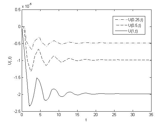
Figure 1. Damping of the oscillating material: at points $x=0.25,0.5,1$.

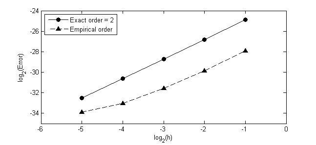
Figure 2. Order of convergence for spatial discretization

References

• [1] K. Adolfsson, M. Enelund, and S. Larsson, Adaptive discretization of fractional order viscoelasticity using sparse time history, Comput. Methods Appl. Mech. Engrg. 193 (2004), 4567–4590.
• [2] K. Adolfsson, M. Enelund, and S. Larsson, Space-time discretization of an integro-differential equation modeling quasi-static fractional-order viscoelasticity, J. Vib. Control 14 (2008), 1631–1649.
• [3] K. Adolfsson, M. Enelund, S. Larsson, and M. Racheva, Discretization of integro-differential equations modeling dynamic fractional order viscoelasticity, LNCS 3743 (2006), 76–83.
• [4] G.A. Baker, Error estimates for finite element methods for second order hyperbolic equations, SIAM J. Numer. Anal. 13 (1976), 564–576.
• [5] W. Bangerth, M. Geiger, and R. Rannacher, Adaptive Galerkin finite element methods for the wave equation, CMAM. 10 (2010), 3–48.
• [6] C. Carstensen, An adaptive mesh-refining algorithm allowing for an $H^{1}$ stable $L^{2}$ projection onto Courant finite element spaces, Constr. Approx. 20 (2004), 549–564.
• [7] S. Larsson and F. Saedpanah, The continuous Galerkin method for an integro-differential equation modeling dynamic fractional order viscoelasticity, IMA J. Numer. Anal. 30 (2010), 964–986.
• [8] Y. Lin, V. Thomée, and L. B. Wahlbin, Ritz-volterra projections to finite-element spaces and application to integro-differential and related equations, SIAM J. Numer. Anal. 28 (1991), 1047–1070.
• [9] M. K. Warby M. Karamanou, S. Shaw and J. R. Whiteman, Models, algorithms and error estimation for computational viscoelasticity, Comput. Methods Appl. Mech. Engrg. 194 (2005), 245–265.
• [10] W. McLean and V. Thomée, Numerical solution via laplace transforms of a fractional order evolution equation, J. Integral Equations Appl. 22 (2010), 57–94.
• [11] A. Pazy, Semigroups of Linear Operators and Applications to Partial Differential Equations, Springer-Verlag, 1983.
• [12] J. E. M. Rivera and G. P. Menzala, Decay rates of solution to a von Kármán system for viscoelastic plates with memory, Quart. Appl. Math. Eng. LVII (1999), 181–200.
• [13] B. Riviére, S. Shaw, and J. R. Whiteman, Discontinuous Galerkin finite element methods for dynamic linear solid viscoelasticity problems, Numer. Methods Partial Differential Equations 23 (2007), 1149–1166.
• [14] F. Saedpanah, A posteriori error analysis for a continuous space-time finite element method for a hyperbolic integro-differential equation, BIT Numer. Math., to appear, Available at Cornell University Library, arXiv:1205.0159.
• [15] by same author, Well-posedness of an integro-differential equation with positive type kernels modeling fractional order viscoelasticity, Cornell University Library, arXiv:1203.4001.
• [16] by same author, Optimal order finite element approximation for a hyperbolic integro-differential equation, BIMS 38 (2012), 447–459.
• [17] A. Schädle, M. López-Fernández, and Ch. Lubich, Adaptive, fast, and oblivious convolution in evolution equations with memory, SIAM J. Sci. Comput. 30 (2008), 1015–1037.
• [18] S. Shaw and J. R. Whiteman, A posteriori error estimates for space-time finite element approximation of quasistatic hereditary linear viscoelasticity problems, Comput. Methods Appl. Mech. Engrg. 193 (2004), 5551–5572.
• [19] I. H. Sloan and V. Thomée, Time discretization of an integro-differential equation of parabolic type, SIAM J. Numer. Anal. 23 (1986), 1052–1061.
• [20] V. Thomée, Galerkin Finite Element Methods for Parabolic Problems, second ed., Springer Series in Computational Mathematics, vol. 25, Springer-Verlag, 2006.