Toward a Spectroscopic Census of White Dwarfs Within
40 parsecs of the Sun

Abstract

We present the preliminary results of a survey aimed at significantly increasing the range and completeness of the local census of spectroscopically confirmed white dwarfs. The current census of nearby white dwarfs is reasonably complete only to about 20 parsecs of the Sun, a volume that includes around 130 white dwarfs, a sample too small for detailed statistical analyses. This census is largely based on follow-up investigations of stars with very large proper motions. We describe here the basis of a method that will lead to a catalog of white dwarfs within 40 parsecs of the Sun and north of the celestial equator, thus increasing by a factor of 8 the extent of the northern sky census. White dwarf candidates are identified from the SUPERBLINK proper motion database, allowing us to investigate stars down to a proper motion limit $\mu>40$ mas yr^-1, while minimizing the kinematic bias for nearby objects. The selection criteria and distance estimates are based on a combination of color-magnitude and reduced proper motion diagrams. Our follow-up spectroscopic observation campaign has so far uncovered 193 new white dwarfs, among which we identify 127 DA (including 9 DA+dM and 4 magnetic), 1 DB, 56 DC, 3 DQ, and 6 DZ stars. We perform a spectroscopic analysis on a subsample of 84 DAs, and provide their atmospheric parameters. In particular, we identify 11 new white dwarfs with spectroscopic distances within 25 pc of the Sun, including 5 candidates to the $D<20$ pc subset.

I. Introduction

Statistics of the local white dwarf population, such as the space density, luminosity function, and mass distribution, are fundamental tools for understanding the evolution of the Galactic stellar populations and quantifying their ages (Oswalt et al. 1996, Leggett et al. 1998). Because of their low luminosities, obtaining a large and complete census of white dwarfs within a well-defined volume remains a challenge. The best volume that can be defined for a census of low-luminosity objects is the solar neighborhood, which alleviates the need for deep surveys, and also allows one to map out the sample in velocity space using readily available proper motions.

A catalog and analysis of the sample of white dwarfs within 20 pc of the Sun were presented by Holberg et al. (2002), and later refined by Holberg et al. (2008) and Sion et al. (2009). In light of these studies, the current census of nearby white dwarfs is believed to be 80% complete, and contains 127 white dwarfs (Sion et al., 2009). Every white dwarf suspected to lie within 20 parsecs of the Sun was analyzed in greater detail by Giammichele et al. (2012), and 130 members ended up in their sample of local white dwarfs. Even if one assumes that the local sample is complete, the size of the sample is too small for detailed statistical analyses, and there is a need to extend the census and obtain a complete sample of white dwarfs from a larger volume. Such an effort was undertaken by Subasavage et al. (2009, and earlier references within) by measuring trigonometric parallaxes for new white dwarfs that are candidates of the 25 pc sample, as part of their DENSE project focused on objects in the southern hemisphere. Holberg et al. (2011) also announced that the complete sample of white dwarfs will be extended to 25 parsecs, thus doubling the volume of the local sample. Based on the space density of white dwarfs known within 10 pc of the Sun, Subasavage et al. (2009) estimated that the census of white dwarfs within 25 pc and with accurate trigonometric parallaxes is only $\sim 40\%$ complete, and if we extend this horizon a little further — to 40 pc for instance — the census of white dwarfs remains largely incomplete.

Nearby white dwarfs have been traditionally discovered in catalogs of stars with high proper motions. Major contributions have been made, for instance, by Luyten (1979a, b), Giclas (1971), and Giclas et al. (1978), who identified a significant number of faint, blue, high proper motion stars, and their pioneer work is still useful to today’s astronomers. Indeed, in the first study dedicated to building a complete census of the local sample of white dwarfs by Holberg et al. (2002), LHS, G, and GD objects form an important fraction of the 109 objects reported in that sample. Major contributions to the completeness of the local white dwarf sample also come from the work of Vennes & Kawka (2003), Kawka et al. (2004), and Kawka & Vennes (2006), who surveyed the revised NLTT catalog of Salim & Gould (2003), and in particular, identified eight new white dwarfs lying within 20 pc of the Sun. The contribution of Farihi et al. (2005) is also worth mentioning in this effort, as well as those of Subasavage et al. (2007, 2008, 2009), and Sayres et al. (2012), aimed at completing the 25 pc sample.

But in order to extend the volume of our complete sample of white dwarfs, the first step is to identify nearby stars with smaller proper motions, the coolest ($T_{\rm eff}\sim 3500$ K) of which are extremely faint due to the intrinsic small radius of white dwarfs. With the goal to improve the statistics of the local white dwarf population, we have been hunting for white dwarfs in the SUPERBLINK catalog. This catalog, which is based on a re-analysis of the Digitized Sky Surveys — with its 20-45 yr baseline — is at least 95% complete for the entire northern sky down to $V=19.0$, with a very low rate of spurious detection. It thus constitutes an ideal database from which to search for faint, high proper motion objects such as nearby white dwarfs. Also, because of its low proper motion limit ($\mu>0\farcs 04$ yr^-1), the SUPERBLINK sample effectively eliminates the kinematic bias for stars in the immediate vicinity of the Sun, which is a known limitation of traditional catalogues such as the LHS catalog ($\mu>0\farcs 5$ yr^-1; Luyten 1979a) and the NLTT catalog ($\mu>0\farcs 18$ yr^-1; Luyten 1979b). Hence, the SUPERBLINK catalog also represents a powerful tool for the study of the solar neighborhood. Searching this database should provide a complete sample of white dwarfs to a much larger distance limit.

Also, the high completeness and deep magnitude limit of SUPERBLINK allows the detection of all white dwarfs down to the luminosity function turnoff, which occurs at $L/L_{\odot}\simeq 10^{-4}$ (Fontaine et al., 2001), up to a relatively large distance. For a 0.6 $M_{\odot}$ white dwarf with a pure hydrogen atmosphere, for instance, this corresponds to $T_{\rm eff}=5000$ K, or $M_{V}$=15.23. The limiting magnitude of $V=19$ implies that SUPERBLINK should be detecting all white dwarfs down to the luminosity function turnoff to a distance of 56.7 pc from the Sun. The main question is what fraction of these stars are expected to have proper motions above the SUPERBLINK limit of $\mu>0\farcs 04$ yr^-1. Assuming that the distribution of velocities for white dwarfs to be the same as that of main-sequence stars in the vicinity of the Sun, we can use Figure 1 of Lépine & Gaidos (2011), which shows the kinematic selection effects of SUPERBLINK by illustrating the fraction of stars in the Hipparcos catalog that would be selected with a proper motion cut of $\mu>0\farcs 04$ yr^-1 up to a given distance. At 56.7 pc, more than 90% of the stars are detected. This minimal kinematic bias therefore allows one to detect most white dwarfs down to the luminosity function turnoff, and to perform a complete statistical analysis on a sample $\sim 10$ times larger than the current 20 pc census.

The interest in the local population of white dwarf stars in not only statistical, but also astrophysical. Indeed, probing the solar neighborhood allows the detection of faint, cool stars that would remain undetected at larger distances. Since the cool end of the white dwarf luminosity function is incomplete, obtaining a reliable estimate of the space density of white dwarf stars and comparing the luminosity function to models remains a challenge. The completion of the cool end of the white dwarf luminosity function would allow the accurate determination of the Galactic age and the verification of the white dwarf cooling theory. Furthermore, many cool white dwarfs are peculiar (Giammichele et al., 2012), and it is among them that we can expect to find transition objects that would allow us to establish the link between the different spectral types and to achieve a better understanding of the white dwarf spectral evolution. The catalog of Holberg et al. (2008) contains a large number of stars of particular astrophysical interest. For a detailed description of these stars, see Giammichele et al. (2012) and references therein. It is expected that surveys at 25 and 40 parsecs will unveil an even larger number of such key objects.

In this paper, we search the SUPERBLINK catalog to extend significantly the census of white dwarfs in the solar neighborhood. Lépine & Shara (2005) have shown how reduced proper motion diagrams constructed from the SUPERBLINK catalog can produce a large number of white dwarf candidates. We present here a more detailed search and identification of these white dwarfs through a large spectroscopic follow-up program. Our specific goal is to obtain spectral confirmation of all suspected white dwarfs within 40 parsecs of the Sun. Given the enormous amount of data and limited telescope access, we restrict ourselves to the northern part of the sky. The first step of this spectroscopic survey consists in the identification, observation, and classification of the white dwarf candidates. In Section 2, we present the catalog from which the candidates are obtained. We detail our selection method in Section 3, as well as distance estimates and candidate list in Section 4. Section 5 describes the results of our spectroscopic observation campaign, while a preliminary spectroscopic analysis, including the determination of atmospheric parameters, is provided in Section 6. Finally, a discussion follows in Section 7. A more thorough model atmosphere analysis of the atmospheric parameters of our complete survey of new white dwarfs within 40 parsecs will be reported in subsequent papers.

II. Proper Motion and Photometric Database

Our white dwarf candidates are identified from the SUPERBLINK catalog of stars with proper motions $\mu>40$ mas yr^-1. This catalog, based on a re-analysis of the Digitized Sky Surveys (which include POSS-I and POSS-II plate scans), is estimated to be $>95\%$ complete in the northern hemisphere down to a visual magnitude of $V=19$, but extends to $V\sim 20$ in many areas of higher Galactic latitudes. The current version of the catalog comprises 2,283,540 objects, all designated by the letters “PM I” followed by 10 characters based on the right ascension ($\alpha$) and declination ($\delta$) of the object. The basic search algorithm is described in Lépine et al. (2002), while quality control procedures, including cross-correlation with other catalogs and the compilation of astrometric and photometric results, are discussed at length in Lépine & Shara (2005) and Lépine & Gaidos (2011). A complete list of 61,977 northern stars with $\mu>150$ mas yr^-1 has already been published in Lépine & Shara (2005). We provide below a brief summary of the astrometric and photometric entries given in the current SUPERBLINK catalog.

Table 1Available Photometric Data

Catalog	Version	Bands	Counterparts	Reference
2MASS	$-$	$JHK_{S}$	1,472,665	Skrutskie et al. (2006)
SDSS	DR6	$ugriz$	345,958	Adelman-McCarthy et al. (2008)
Hipparcos, Tycho-2	$-$	$B_{T},V_{T}$	118,000	van Leeuwen (2007)
				Høg et al. (2000)
USNO-B1.0	$-$	$B_{J},R_{F},I_{N}$	1,567,461	Monet et al. (2003)
GALEX	GR6	FUV, NUV	143,806	Gil de Paz et al. (2009)

II.1. Astrometry

SUPERBLINK provides coordinates on the International Celestial Reference System for the 2000.0 epoch. For stars catalogued in Hipparcos, the positions are extrapolated to the 2000.0 epoch from the values given in van Leeuwen (2007), which are listed for the 1991.25 epoch. Likewise, those not in Hipparcos but listed in Tycho-2 have their positions extrapolated from the proper motions listed in Tycho-2, and if a star has a counterpart in 2MASS (Cutri et al., 2003), its position is extrapolated from the position of the 2MASS counterpart. Finally, coordinates for stars without a Hipparcos or 2MASS counterparts are calculated by SUPERBLINK from the position of the stars on the POSS-II scans. The coordinates of those stars are thus less accurate but are generally within a few arcseconds (see Lépine & Shara 2005 for details).

SUPERBLINK also lists proper motions for each entry, tabulated from three sources. When available, proper motions are taken from the Hipparcos catalog (van Leeuwen, 2007) or from the Tycho-2 catalog (Høg et al., 2000). Otherwise, the proper motions listed are those measured in the SUPERBLINK proper motion survey, based on the Digitized Sky Survey images. SUPERBLINK ends up providing proper motions for more than 2 million stellar objects, and in particular, a total of 1,567,461 stars with $\delta>0$. From now on, when we mention the SUPERBLINK database, we refer to the northern part of the catalog.

II.2. Photometric Data

The construction of reduced proper motion diagrams requires, in addition to proper motion measurements, a set of photometric data in order to estimate the color of each star. Fortunately, the cross-correlation of SUPERBLINK with other catalogs not only allows coordinates and proper motions to be measured with more accuracy, but it also provides a useful set of photometric data covering a large portion of the electromagnetic spectrum. We describe these data in turn, and a summary is provided in Table 1.

The Two Micron All Sky Survey (2MASS) Point Source Catalog (Skrutskie et al., 2006) represents an excellent source of near-infrared magnitudes for our targets in SUPERBLINK since the 2MASS survey covers the whole sky and is complete down to $J\sim 16.5$. Lépine & Shara (2005, see their Figure 30) successfully showed that white dwarfs in SUPERBLINK could easily be separated from other stellar populations in a $H_{V}$ vs $V-J$ reduced proper motion diagram. For the present study, we used a version of the SUPERBLINK catalog in which 2MASS counterparts had already been found and assigned to 1,472,665 of the stars ($\sim 94\%$), with the remainder having no detectable counterpart in 2MASS. These infrared $J$, $H$, and $K_{S}$ magnitudes have a 0.02-0.03 mag accuracy down to 13th magnitude, and point sources are detected with S/N better than 10 for stars brighter than $J=15.9$, $H=15.0$, and $K_{S}=14.3$ (Skrutskie et al., 2006).

The Sloan Digital Sky Survey (SDSS) also represents a useful source of photometric data, with $ugriz$ photometry from the Data Release 6 (Adelman-McCarthy et al., 2008) for 345,958 counterparts in the SUPERBLINK catalog. The SDSS magnitudes have photometric uncertainties of roughly 1% in the $griz$ bands and 2% in $u$ (Padmanabhan et al., 2008). This is by far the most accurate optical photometry available in our study, and will be especially useful to identify white dwarfs in the SUPERBLINK catalog.

Optical photometry in the blue ($B_{T}$) and in the visual ($V_{T}$) range are also extracted for 118,475 stars with counterparts in the Hipparcos and Tycho-2 catalogs. Additional optical photometry was also obtained from the USNO-B1.0 database (Monet et al., 2003), providing photographic magnitudes for the totality of the catalog, i.e. 1,567,461 objects. However, for some entries, the photometry is available only for one or two bands. More specifically, $B_{J}$ magnitudes are available for 1,390,471 objects, $R_{F}$ magnitudes for 1,405,840, and $I_{N}$ magnitudes for 912,550 objects. The blue $B_{J}$ magnitudes are extracted mostly from scans of IIIaJ plates from the Palomar Sky Surveys (POSS-I, POSS-II) and the Southern ESO Schmidt (SERC) Survey, the red $R_{F}$ magnitudes are extracted from scans of IIIaF plates from POSS-I and POSS-II and also from the Anglo-Australian Observatory red survey (AAO-red), while the near-infrared $I_{N}$ magnitudes are extracted from the IVn plates from POSS-II and SERC. The $B_{T}$ and $V_{T}$ magnitudes are more accurate (0.1 mag or better) than the photographic magnitudes (typically 0.5 mag), but they are available only for the brightest stars in SUPERBLINK, while photographic magnitudes are available for every object.

Finally, we also searched the sixth data release (GR6) of the GALEX database (Gil de Paz et al., 2009) and identified 147,096 counterparts to the SUPERBLINK objects (for a $5\farcs 0$ search radius). The corresponding far-ultraviolet (FUV, 1350-1780 Å) and near-ultraviolet (NUV, 1770-2730 Å) magnitudes are particularly useful for the identification of blue objects, and in particular white dwarf stars.

III. Selection of the Candidates Based on Reduced Proper Motion Diagrams

Reduced proper motion diagrams (RPMD) are a particularly efficient tool to identify white dwarf candidates with known proper motions (see, for instance, Knox et al. 1999, Oppenheimer et al. 2001, Vennes & Kawka 2003, Carollo et al. 2006, Kilic et al. 2006). The reduced proper motion of an object is defined as $H_{m}=m+5\log\mu+5$, where $m$ is the apparent magnitude in some bandpass and $\mu$ is the proper motion measured in arcseconds per year. The reduced proper motion is analogous to the absolute magnitude $M_{m}=m+5\log\pi+5$, where the trigonometric parallax $\pi$ is replaced with the proper motion $\mu$ of the object. A reduced proper motion diagram is thus similar to a color-magnitude diagram, and white dwarfs occupy a similar location in the diagram, i.e. the bottom-left region. Furthermore, using the tangential velocity $v_{\rm tan}=4.74\,\mu\pi^{-1}$ in units of $\rm{km}~{}s^{-1}$ instead of the proper motion, we obtain $H_{m}=M_{m}+5\log{v_{\rm tan}}-3.38$, and each star population can be isolated based on the mean value of its tangential velocity.

One major problem with the identification of white dwarf candidates using reduced proper motion diagrams is the contamination of the white dwarf region by other stellar populations, and by high-velocity subdwarfs in particular. Vennes & Kawka (2003) showed, however, that this contamination can be substantially reduced by the inclusion of a criterion based on $V-J$. Similarly, Kilic et al. (2006) demonstrated that reduced proper motion diagrams are efficient for detecting cool white dwarfs only when the measured proper motions of all stellar populations are reliable, since subdwarfs with inaccurate proper motions can contaminate the other stellar populations, and notably the white dwarf region of the diagram. SUPERBLINK has an estimated false detection level of less than $1\%$ down to $V=19$, but the false detection rate increases significantly for fainter sources. In our selection criteria, we thus restrict our search to that stars with $V<19$. Fortunately, SUPERBLINK has a very high level of completeness for $V<19$, exceeding $98\%$ for most of the sky. We are thus confident that we can easily identify a significant fraction of the nearby white dwarfs using this technique. The next sections describe the four reduced proper motion diagrams we used to identify white dwarf candidates in SUPERBLINK, in an effort to take advantage of the whole set of photometric information available. The order in which these are presented follows the order of their estimated efficiency at isolating the white dwarf population, starting with the most efficient one.

III.1. RPMD Using $ugriz$ Photometry

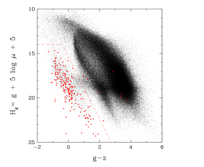
Figure 1.— Reduced proper motions diagram ($H_{g},g-z$) for the 345,958 stars in the SUPERBLINK catalog ($\mu>40$ mas yr^-1) with counterparts in the SDSS 6th Data Release. The red dashed lines show the limits used to define the location of the white dwarfs. These limits include 4929 white dwarf candidates, i.e. $1.4\%$ of the sample of SUPERBLINK stars with SDSS photometry. The spectroscopically confirmed white dwarfs from the WD Catalog are shown as large red dots.

We present in Figure 1 the $H_{g}$ vs $g-z$ reduced proper motion diagram constructed from the 345,958 SUPERBLINK objects in the northern hemisphere with $ugriz$ photometry available from the 6th Data Release of the Sloan Digital Sky Survey. As a result of the relatively high accuracy of the SDSS magnitudes, the white dwarf population is particularly well separated from the other populations in this diagram.

To verify the accuracy of our procedure, we also display as red dots in Figure 1 the sample of white dwarfs taken from the 2008 May electronic version of the Catalogue of Spectroscopically Identified White Dwarfs (McCook & Sion, 1999, hereafter WD Catalog) with $\delta>0$ also found in SUPERBLINK and with $g$ and $z$ photometry available. We first note that 191 spectroscopically confirmed white dwarfs lie in the expected region near the bottom left of the diagram, and that a small number of white dwarfs are color outliers. More precisely, 3 white dwarfs overlap the subdwarf region, and 4 are found in the redder, main sequence portion of the diagram. Two of these are actually binary systems: 0855+604.1 is a DBQ (Greenstein, 1969) and 0855+604.2 is a DCE? (Eggen & Greenstein, 1965), while 1133+358 is an unresolved DC+dM (Greenstein, 1976).

Fortunately, there are enough spectroscopically identified white dwarfs that are well separated from the other populations to allow us to define selection criteria for the white dwarf area. These criteria are defined by the need to include as many white dwarf candidates as possible, while trying to keep the contamination from subdwarfs to a minimum. As a general criterion, the area occupied by the white dwarfs must include at least 80% of the spectroscopically confirmed white dwarfs. In the present case, this limit between the halo subdwarfs and the white dwarf area is defined by the following linear equation $H_{g}=3.5(g-z)+16.5$. The slope and y-intercept are chosen in a very conservative manner, and include 96% of the WD Catalog sample with measured $ugriz$ photometry. The reason why we recover almost all white dwarfs from the WD Catalog is that the known white dwarf population is well separated in this reduced proper motion diagram, and only a few objects are color outliers. However, in the upper part of the diagram ($H_{g}\lesssim 14$) there is again some confusion between the different stellar populations defined by our linear equation, so we simply apply an additional cutoff at $H_{g}=14$ based on the known white dwarf population, in order to keep the contamination to a minimum. These adopted selection criteria for the $H_{g}$ vs $g-z$ diagram are displayed in Figure 1. Out of the 345,958 SUPERBLINK stars with a counterpart in the 6th Data Release of the SDSS, about 4929 fall within the white dwarf selection limits. This number represents 1.4% of the stars in the catalog with SDSS photometry, or $0.5\%$ of the total number of objects in SUPERBLINK.

III.2. RPMD Using GALEX Photometry

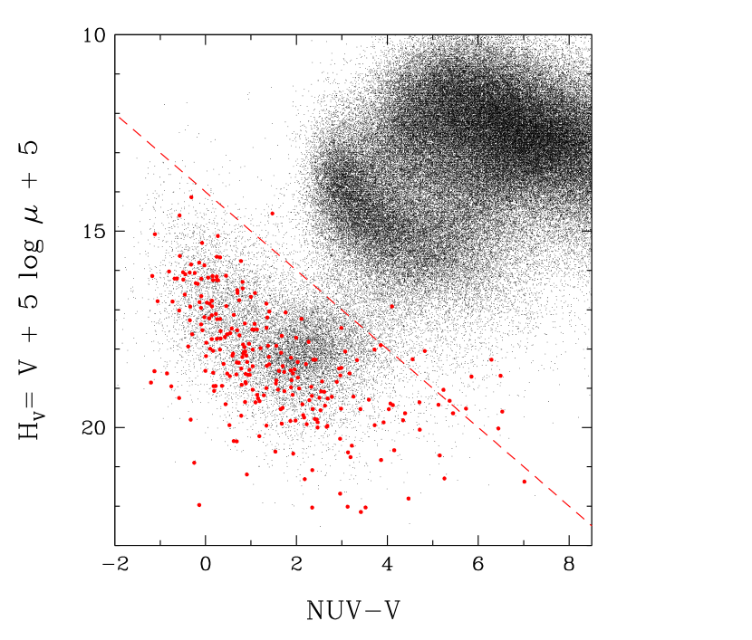
Figure 2.— Reduced proper motions diagram ($H_{V}$, ${\rm{NUV}}-V$) for the 147,096 stars in the SUPERBLINK catalog ($\mu>40$ mas yr^-1) with counterparts in the 6th Data Release of the GALEX survey. The red dashed line shows the limits used to define the location of the white dwarfs. This limit includes 19,150 white dwarf candidates, i.e. $12.7\%$ of the sample of SUPERBLINK stars with GALEX photometry. The spectroscopically confirmed white dwarfs from the WD Catalog are shown as large red dots.

White dwarf stars are generally hotter than main sequence or subdwarf stars, and since their atmospheres are usually devoid of heavy elements that could absorb the UV flux, they are moderately strong UV emitters and can easily be distinguished from non-degenerate stars in a reduced proper motion diagram built from GALEX photometry. We present in Figure 2 the $H_{V}$ vs ${\rm{NUV}}-V$ diagram containing 147,096 stars in SUPERBLINK with NUV magnitudes measured by GALEX. NUV magnitudes are used in this diagram since they are available for a much larger number of stars than the FUV magnitudes. No corrections are applied for interstellar reddening, since according to the characterization of the Local Bubble of Reis et al. (2011), the smallest distance to the wall of dust that causes extinction ($E(b-y)\geq 0.040$) is $\sim 80$ pc. The reddening should thus not affect the white dwarf candidates of the local sample.

Here and in the following diagrams, the $V$ magnitudes are estimated from the relation

$$V=B_{J}-0.46(B_{J}-R_{F})$$ (1)

as recommended by Lépine & Shara (2005), where $B_{J}$ and $R_{F}$ are photographic magnitudes taken from the USNO-B1.0 catalog. These estimated $V$ magnitudes are believed to be accurate to $\pm 0.5$ mag (Lépine & Shara, 2005). As mentioned earlier, while $V_{T}$ magnitudes from the Tycho-2 catalog are more accurate than photographic magnitudes, they are only available for a small number of SUPERBLINK objects, whereas $B_{J}$ and $R_{F}$ exist for the majority of our targets. Hence, despite the relatively large uncertainties of the $V$ magnitudes employed here, they have the advantage of being available for most of the entries in SUPERBLINK.

As in Figure 1, the spectroscopically confirmed white dwarfs from the WD Catalog are also shown in red. Here, a total of 13 spectroscopically confirmed white dwarfs white dwarfs are scattered in areas normally occupied by other stellar populations. Most of these objects are cool degenerates, including 9 DA, 2 DC, 1 DZ (1705+030, Greenstein 1984) and 1 DQ star (1105+412, Koester and Knist, 2006). Most likely, these have very little UV flux and thus inaccurate NUV magnitudes.

We define the slope and y-intercept of the line that characterizes the white dwarf region with the same criteria as before. Also, since the halo subdwarfs and main sequence stars are generally not as bright in the UV as white dwarfs are, there is no need to apply any further cutoff in $H_{V}$. Therefore, to be considered a white dwarf candidate, a star must have a reduced proper motion larger than $H_{V}=({\rm NUV}-V)+14$. With this limit, $94\%$ of the white dwarfs from the WD Catalog with measured NUV photometry are recovered. Finally, if this criterion is applied to the 147,096 SUPERBLINK objects with both NUV and $V$ magnitudes, we obtain a sample of 19,150 white dwarf candidates, which represent 12.7% of the stars with GALEX photometry in SUPERBLINK, or $2.0\%$ of the complete catalog.

III.3. RPMD Using 2MASS Photometry

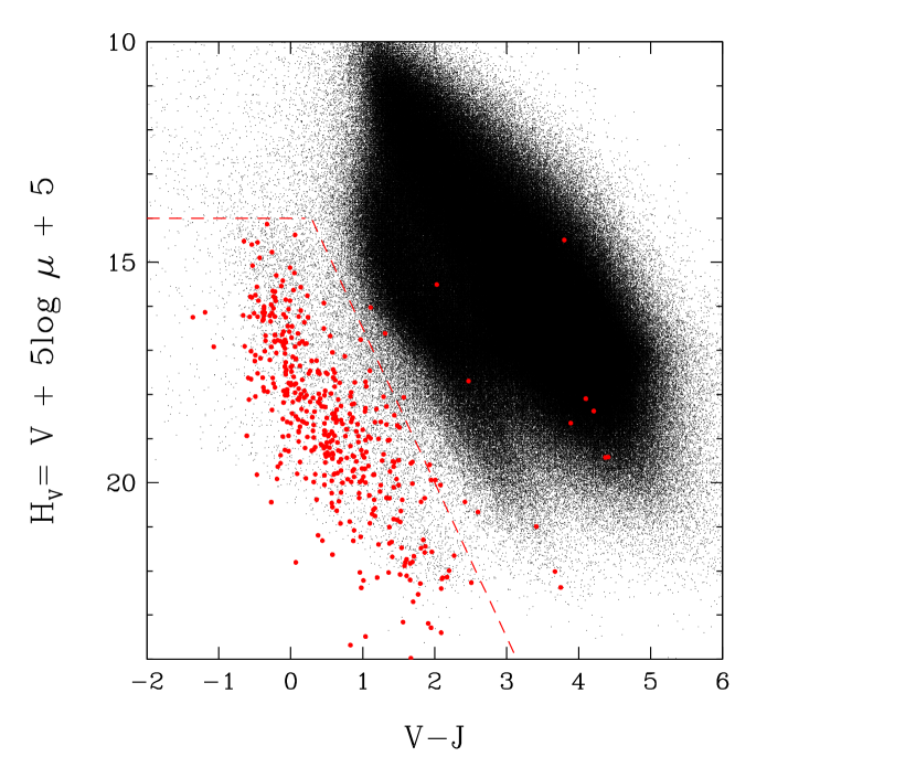
Figure 3.— Reduced proper motions diagram ($H_{V},V-J$) for the 1,265,733 stars in the SUPERBLINK catalog ($\mu>40$ mas yr^-1) with counterparts in the 2MASS catalog and for which an estimation of the $V$ magnitude was possible. The red dashed lines show the limits used to define the location of the white dwarfs. These limits include 16,977 white dwarf candidates, i.e. $1.3\%$ of the initial sample. The spectroscopically confirmed white dwarfs from the WD Catalog are shown as large red dots.

As discussed above, the reduced proper motion diagram in $H_{V}$ vs $V-J$, displayed in Figure 30 of Lépine & Shara (2005), showed that nearly 2000 white dwarfs could be identified in the SUPERBLINK catalog of stars with proper motions $\mu>150$ mas yr^-1. Since the SUPERBLINK catalog now includes stars with $\mu>40$ mas yr^-1, and because a significant fraction of its entries has a counterpart in the 2MASS catalog, such a diagram has an even greater potential for identifying white dwarf stars. The resulting $H_{V}$ vs $V-J$ diagram is shown in Figure 3, and contains 1,265,733 stars from SUPERBLINK with $J$ magnitudes taken from 2MASS as well as $B_{J}$ and $R_{F}$ magnitudes from the USNO-B1.0 catalog. Here again, the $V$ magnitudes are obtained from the empirical calibration given by Equation (1).

The comparison with the spectroscopically confirmed white dwarfs from the WD Catalog reveals 20 objects that fall in a region to the right of that occupied by the bulk of white dwarfs. Among them, there are 9 DA, 4 DC, 1 DQ, and 1 DZ star. This diagram also includes the largest number of multiple-star systems identified so far. Indeed, we find four WD+dM systems, a DB+DC binary (2058+342, Farihi 2004), and 0023+388, the triple star system discussed earlier.

Applying similar criteria as before, the white dwarf candidates are selected from Figure 3 if their reduced proper motion is larger than $H_{V}=3.5(V-J)+13$, with a cutoff of $H_{V}>14$. These limits, displayed in Figure 3, recover 86% of the white dwarfs from the WD Catalog listed in SUPERBLINK and for which 2MASS and photographic magnitudes are available. This defines a sample of 16,977 white dwarf candidates out of the 1,265,733 objects in the initial SUPERBLINK sample with 2MASS photometry, or a fraction of $1.3\%$ (0.23% of the total initial sample).

III.4. RPMD Using Photographic Magnitudes

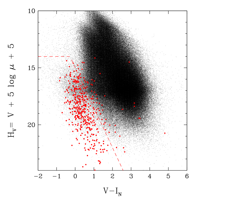
Figure 4.— Reduced proper motions diagram ($H_{V},V-I_{N}$) for the 878,847 stars in the SUPERBLINK catalog ($\mu>40$ mas yr^-1) with counterparts in the USNO-B1.0 catalog for all three $B_{J}$, $R_{F}$ and $I_{N}$ photographic magnitudes. The red dashed lines show the limits used to define the location of the white dwarfs. These limits include 20,862 white dwarf candidates, i.e. $2.4\%$ of the initial sample. The spectroscopically confirmed white dwarfs from the WD Catalog are shown as large red dots.

Even if USNO-B1.0 photographic magnitudes are less accurate than CCD photometry obtained in recent large surveys such as SDSS, they have the advantage of covering the whole sky, and are thus available for all 1.6 million SUPERBLINK objects. We present in Figure 4 the reduced proper motion diagram in $H_{V}$ vs $V-I_{N}$ constructed with $V$ as defined by Equation (1). To be included in this diagram, photographic $B_{J}$, $R_{F}$, and $I_{N}$ magnitudes must all be available for each object. However, as discussed by Lépine & Shara (2005), not all USNO-B1.0 entries have magnitude information in all three bands. Whenever possible, Lépine & Shara tried to combine data if a USNO-B1.0 star appeared as more than one entry, but some sources remained without information for one or more bands. As a result, Figure 4 includes $878,847$ stars out of the $1,567,461$ entries in SUPERBLINK with at least one photographic magnitude in USNO-B1.0.

In Figure 4, the separation between the white dwarf and subdwarf populations is not as well defined as in the other reduced proper motion diagrams. The $V$ and $I_{N}$ filters are indeed too close in wavelength to allow an efficient separation of the two populations, as was the case with $V-J$ or $g-z$, for instance. We also have to consider the fact that there is an uncertainty of $\pm 0.5$ mag in both $V$ and $I_{N}$, which adds to the dispersion in $V-I_{N}$. The comparison of the white dwarfs in the WD Catalog displayed in Figure 4 with those in Figure 3 using $V-J$ reveals that most of the 55 outliers in $V-I_{N}$ are also outliers in $V-J$, the difference between the two diagrams being that there is a larger concentration of outliers in $V-I_{N}$ near the white dwarf locus. Once again, the measurement uncertainty in $V-I_{N}$ is to blame. All of the interesting outliers have been discussed in the preceding sections and will not be repeated here.

Despite this large contamination, we must still define some selection criteria, and as before, the slope and y-intercept of the limit between white dwarfs and halo subdwarfs is chosen to include $80\%$ of the white dwarfs from the WD Catalog; a lower limit in $H_{V}$ is also defined. Using these criteria, the white dwarf candidates are selected from Figure 4 if their reduced proper motion is larger than $H_{V}=3.5(V-I_{N})+13$, with a cutoff of $H_{V}>14$. This time, since the contamination is much larger than in previous reduced proper motion diagrams, a more conservative cut must be used, and no more than $80\%$ of the white dwarfs from the WD Catalog are recovered. We finally end up with 20,862 white dwarf candidates out of the $878,847$ SUPERBLINK objects in the original sample with USNO photometry, or a fraction of $2.2\%$ of the total catalog.

Combining the results from all four reduced proper motion diagrams, we obtain a total of 20,862 white dwarf candidates, since all of them have USNO photographic magnitudes, but only a fraction of them have data available in other photometric systems. Some of these candidates, however, can be found in up to four reduced proper motion diagrams. At this point, each candidate can be assigned an order of priority depending on the quality of the photometry used for its identification.

III.5. A Priority Approach

For each given star, data can be available for up to four photometric systems and their corresponding reduced proper motion diagrams. Thus, it is possible that a star could be within the white dwarf region defined by our selection criteria in one diagram and outside in another diagram. We must therefore decide which photometric system should be prioritized to decide whether or not a star should be included in our final list of $\sim 21,000$ white dwarf candidates. For instance, $ugriz$ magnitudes should take precedence over photographic magnitudes, since the former are much more accurate. In the following, we establish the order of priority for our four photometric systems, based on their degree of photometric accuracy.

SDSS magnitudes have a relatively high degree of accuracy and cover a wavelength range that allows an efficient separation of the white dwarfs from the other stellar populations, as discussed above. The reduced proper motion diagram based on $ugriz$ magnitudes is arguably the most accurate, and it is therefore given the highest priority. However, a comparison of our preliminary list of white dwarf candidates based on $ugriz$ data with those found in the literature shows a significant contamination from subdwarfs. Kawka et al. (2004) successfully reduce this contamination by including a color-color criterion to their reduced proper motion cut, namely $(V-J)<3.28(J-H)-0.75$. But such limits also get rid of the white dwarfs with red, main-sequence companions, which we would like to include. Also, as observed by Kilic et al. (2006) and Sayres et al. (2012), any uncertainty in the proper motion measurements can lead to contamination. Also, spurious proper motions are possible for stars near the faint magnitude limit of the SUPERBLINK. With all these considerations in mind, we apply on top of the criteria in ($H_{g},g-z$), a criterion inspired by Kawka et al. (2004), but based on Figure 3. It is defined as follows: stars with $V<14$ must also have $H_{V}=3.5(V-J)+13$. This limit on $V$ removes the largest number of known main sequence stars from our list of candidates, while keeping all the known white dwarfs. Applying the criterion in $(H_{V},V-J)$ to fainter candidates results in the elimination of spectroscopically confirmed white dwarfs, so it is not applied to those fainter stars. Finally, using the criteria defined in Section 3.1, combined with those defined in Section 3.3 when $V<14$, we retain a total of 4823 white dwarf candidates. Unfortunately, the SDSS survey, at the epoch of the DR6, only covered about a quarter of the northern sky. Bright stars also tend to be saturated in SDSS, and we need to limit our selection to stars with $u>13$, $g>14$, $r>14$, $i>14$, and $z>12$ (York et al., 2000). Consequently, there is no SDSS counterpart for every star in the SUPERBLINK catalog, and we must therefore rely on other photometric systems to select our targets.

In the absence of SDSS photometric data, GALEX UV photometry is used instead for the selection, whenever it is available. It is our second choice because of the corresponding photometric accuracy as well as the efficiency of the criteria in ${\rm{NUV}}-V$ to separate white dwarfs from other stellar populations. Here, we also apply the ($H_{V},V-J$) criterion for stars with $V<14.0$ in an effort to decontaminate our sample of candidates. The criteria and the method described in Section 3.2 led to the identification of 8092 additional white dwarf candidates. The GALEX survey covers $80\%$ of the sky, with special care taken to avoid the Galactic plane and Magellanic clouds, which could provide excess background flux in the UV.

In the absence of SDSS and GALEX data, 2MASS photometry combined with the criteria defined in Section 3.3 are used to identify 1132 additional white dwarf candidates with $\delta>0$ and $V<14.0$. The 2MASS survey is a precious source of photometric information since it covers practically the whole sky. However, since it is only complete down to $J\sim 16.5$, our fainter targets do not have a 2MASS counterpart. Finally, if there is no SDSS, GALEX, or 2MASS photometry available for a given target, we must rely on photographic magnitudes obtained from the USNO-B1.0 catalog. With the criteria defined in Section 3.4 and for $V<14.0$, we identify an additional list of 6688 white dwarf candidates.

All in all, a total of 20,735 white dwarf candidates are identified with the help of the four reduced proper motion diagrams described in this section. This large number of candidates amply justifies our decision to restrict our search to the northern hemisphere. Moreover, given our interest in establishing a census of white dwarfs in the solar neighborhood within 40 pc of the Sun, we must further restrain our list of candidates by evaluating photometric distances for each object on our target list.

IV. A Sample of White Dwarf Candidates within 40 pc of the Sun

IV.1. Distances from Color-Magnitude Relations

In the absence of trigonometric parallax measurements for most white dwarf candidates in our sample, we must rely on distances estimated using the only information available, which are the apparent magnitudes of each star in a set of bandpasses covering the ultraviolet to the near-infrared. In this section, we estimate photometric distances from the distance modulus, $m-M_{m}=5\log D-5$, where the absolute magnitude $M_{m}$ is determined from theoretical color-magnitude relations combined with a measured color index in some specified photometric system. To do so, we rely on synthetic colors obtained using the procedure outlined in Holberg & Bergeron (2006) based on the improved Vega fluxes taken from Bohlin & Gilliland (2004). These color-magnitude relations are available on our Web site, or upon request on any photometric system. They cover a range of effective temperature between $T_{\rm eff}=1500$ K and 110,000 K and surface gravities between $\log g=6.5$ and 9.5 for hydrogen-rich atmospheres, and between $T_{\rm eff}=3500$ K and 40,000 K and $\log g=7.0$ and 9.0 for helium-rich atmospheres. Note that we now include in our hydrogen models the opacity from the red wing of Ly$\alpha$ calculated by Kowalski & Saumon (2006) and kindly provided to us by P. Kowalski, which is known to affect the flux in the ultraviolet region of the energy distribution. The calculations of absolute magnitudes also require the use of mass-radius relations for white dwarfs, which are based on evolutionary models similar to those described in Fontaine et al. (2001) but with C/O cores, $q({\rm He})\equiv\log M_{\rm He}/M_{\star}=10^{-2}$ and $q({\rm H})=10^{-4}$, which are representative of hydrogen-atmosphere white dwarfs, and $q({\rm He})=10^{-2}$ and $q({\rm H})=10^{-10}$, which are representative of a helium-atmosphere. From these color-magnitude relations at constant $\log g$ values, we can obtain the corresponding relations at constant mass values using the same evolutionary models as described above.

We present below our results on the SDSS, GALEX, and 2MASS photometric systems, as well as on the USNO-B1.0 photographic system. Synthetic colors were calculated from the bandpasses available from the SDSS website and discussed in Fukugita et al. (1996), while the 2MASS filters are described in Cohen et al. (2003) and the transmission functions were taken from the survey website. Similarly, GALEX synthetic colors were calculated from the bandpasses available from the GALEX website and described in Morrissey & GALEX Science Team (2004), and information about the filters for the USNO-B1.0 are given in Monet et al. (2003), and transmission curves are available from the Digitized Sky Survey website.

IV.1.1 $M_{g}$ vs $g-z$ Calibration

Figure 5.— Theoretical color-magnitude relations for pure hydrogen-atmosphere white dwarfs at 0.4, 0.6, and 0.8 $M_{\odot}$ (dashed lines) and for pure helium-atmosphere white dwarfs at 0.6 $M_{\odot}$ (dotted line). The pure hydrogen sequence at 0.6 $M_{\odot}$ is used to determine absolute $M_{g}$ magnitudes for stars with SDSS photometry. Also shown are the 50 white dwarfs from the WD Catalog with available $ugriz$ photometry and trigonometric parallaxes from the Yale Parallax Catalog.

We show in Figure 5 the theoretical $M_{g}$ vs $g-z$ color-magnitude relation for hydrogen-atmosphere white dwarfs at 0.6 $M_{\odot}$ together with similar sequences at 0.4 $M_{\odot}$ and 0.8 $M_{\odot}$, which are representative of the intrinsic mass distribution for DA stars (see, e.g., Gianninas et al. 2011). These are used below to evaluate the accuracy of our color-magnitude calibration. Also shown in Figure 5 is a single 0.6 $M_{\odot}$ helium-atmosphere sequence used to evaluate the influence of the unknown atmospheric composition on the color-magnitude relations. As can be seen, the 0.6 $M_{\odot}$ helium sequence follows closely the corresponding hydrogen sequence in this particular diagram, and it is thus perfectly justified to rely on the hydrogen-rich sequence only to evaluate the photometric distances to our objects.

As an external verification of our color-magnitude relations, we also plot in Figure 5 the 50 spectroscopically confirmed white dwarfs from the WD Catalog that also have trigonometric parallax measurements published in the Yale Parallax Catalog (van Altena et al., 1995) and with SDSS photometry available; we consider here only stars with parallax uncertainties less than 30%. We also distinguish DA and non-DA stars. The absolute magnitudes $M_{g}$ are directly obtained from the distance modulus $M_{g}=g+5\log\pi+5$. Our results show that the observed scatter with respect to the 0.6 $M_{\odot}$ theoretical sequence is entirely consistent with that expected from the intrinsic white dwarf mass distribution, as indicated by the theoretical sequences at 0.4 and 0.8 $M_{\odot}$. This can be tested more quantitatively by measuring the mass of each star directly from the color-magnitude diagram using our theoretical sequences and a simple interpolation scheme. We obtain a mean mass of $\langle M\rangle=0.63$ $M_{\odot}$, with a dispersion of $\sigma(M)=0.20$ $M_{\odot}$, entirely consistent with the photometric mass distribution obtained by Bergeron et al. (2001, see their section 5.3) for the sample of cool white dwarfs with trigonometric parallaxes from the Yale Parallax Catalog, $\langle M\rangle=0.65$ $M_{\odot}$, $\sigma(M)=0.20$ $M_{\odot}$. As also discussed by Bergeron et al., however, the dispersion expected from spectroscopic mass distributions are considerably smaller, typically $\sigma(M)\sim 0.15$ $M_{\odot}$ (see, e.g., Gianninas et al., 2011) due to the increased sensitivity to $\log g$ of the spectroscopic technique over the photometric method based on trigonometric parallax measurements. We thus conclude from this comparison that our $M_{g}$ vs $g-z$ color-magnitude relation is well calibrated.

Finally, we use the $M_{g}$ vs $g-z$ theoretical relation for all white dwarf candidates in our sample with observed $ugriz$ photometry to estimate a photometric distance for each object assuming a hydrogen-atmosphere and a mass of 0.6 $M_{\odot}$, the average mass for white dwarfs. The photometric distances for 4823 white dwarf candidates in our sample, identified from the $(H_{g},g-z)$ reduced proper motion diagram, are estimated in this manner.

IV.1.2 $M_{V}$ vs ${\rm{NUV}}-V$ Calibration

Figure 6.— Same as Figure 5 but for the determination of absolute $M_{V}$ magnitudes for stars with GALEX photometry. Also shown are the 82 white dwarfs from the WD Catalog with available GALEX photometry and trigonometric parallaxes from the Yale Parallax Catalog. The small dots correspond to USNO photographic magnitudes while the larger symbols make use of Johnson $V$ magnitudes.

In an approach similar to that described in the previous section, we use the theoretical relation between the absolute magnitude $M_{V}$ and the color index ${\rm{NUV}}-V$ to determine an absolute magnitude for every object with observed GALEX photometry, assuming a hydrogen atmosphere at 0.6 $M_{\odot}$. We show in Figure 6 the theoretical $M_{V}$ vs ${\rm{NUV}}-V$ color-magnitude relations for the same mass values and atmospheric compositions as above. In contrast with the results from the previous section, the helium sequence starts to differ from the hydrogen sequence at 0.6 $M_{\odot}$ for ${\rm{NUV}}-V$ $>2$, or $T_{\rm eff}<8000$ K, and becomes significantly different for ${\rm{NUV}}-V$ $>4$, or $T_{\rm eff}<6000$ K. However, since we do not expect to identify many white dwarfs cooler than $\sim 6000$ K on the basis of their UV magnitudes, it is justified to rely solely on the pure hydrogen sequence.

Figure 6 also shows the 82 white dwarfs from the WD Catalog observed by GALEX, with trigonometric parallax measurements available in the Yale Parallax Catalog. Since we are mostly interested here in verifying the validity of our color-magnitude relations, we want to use the best photometry available for each star in order to reduce the scatter related to the uncertainty of photographic magnitudes. Hence, in addition to $V$ magnitudes estimated from USNO photographic magnitudes (small dots in Figure 6), we also show the results obtained using apparent $V$ magnitudes measured on the Johnson photometric system, and taken from the literature (larger symbols in Figure 6). This comparison is thus analogous to that shown in Figure 5, and we see once again that the bulk of white dwarfs is well contained between the 0.4 $M_{\odot}$ and 0.8 $M_{\odot}$ theoretical sequences. Performing the same calculations as before, we find a mean mass of $\langle M\rangle=0.67$ $M_{\odot}$ and a dispersion of $\sigma(M)=0.22$ $M_{\odot}$, still consistent with the values obtained by Bergeron et al. (2001).

We finally apply this calibration to all white dwarf candidates identified from the $(H_{V},\rm{NUV}-V)$ reduced proper motion diagram, and estimate photometric distances for 8092 stars with GALEX photometry (but with no SDSS counterparts).

Figure 7.— Same as Figure 5 but for the determination of absolute $M_{V}$ magnitudes for stars with 2MASS photometry. Also shown are the 167 white dwarfs from the WD Catalog with available 2MASS photometry and trigonometric parallaxes from the Yale Parallax Catalog. The small dots correspond to USNO photographic magnitudes while the larger symbols make use of Johnson $V$ magnitudes.

IV.1.3 $M_{V}$ vs $V-J$ Calibration

The theoretical relations between the absolute $M_{V}$ magnitude and color index $V-J$ are shown in Figure 7. Also displayed are the 167 white dwarfs from the WD Catalog for which a trigonometric parallax measurement in the Yale Parallax Catalog and a $V-J$ color index are available (both Johnson $V$ and USNO photographic magnitudes are displayed, as explained in the previous section).

We note again in this figure that most of the points are contained between the 0.4 $M_{\odot}$ and 0.8 $M_{\odot}$ theoretical sequences, with $\langle M\rangle=0.67$ $M_{\odot}$ and $\sigma(M)=0.21$ $M_{\odot}$, and that the hydrogen- and helium-atmosphere sequences agree sufficiently enough to assume a hydrogen-rich composition for all objects in our sample. We obtain the absolute magnitudes and photometric distances for all 1132 white dwarf candidates having counterparts in the 2MASS catalog (but with no SDSS or GALEX counterparts), assuming a hydrogen-atmosphere and a mass of 0.6 $M_{\odot}$.

IV.1.4 $M_{V}$ vs $V-I_{N}$ Calibration

Figure 8.— Same as Figure 5 but for the determination of absolute $M_{V}$ magnitudes for stars with USNO-B1.0 photographic magnitudes. Also shown are the 151 white dwarfs from the WD Catalog with available USNO photographic magnitudes and trigonometric parallaxes from the Yale Parallax Catalog; the small dots correspond to USNO photographic magnitudes while the larger symbols make use of Johnson $V$ magnitudes. The dot-dashed lines represent the 0.5 mag dispersion around the pure hydrogen sequence at 0.6 $M_{\odot}$ estimated from the accuracy of the $B_{J}$, $R_{F}$, and $I_{N}$ magnitudes.

Figure 8 displays our last color-magnitude relation, that between $M_{V}$ and the photographic color index $V-I_{N}$. Also shown are the 151 white dwarfs from the WD Catalog with trigonometric parallax measurements in the Yale Parallax Catalog and $V-I_{N}$ color indices available. Again, both Johnson $V$ and USNO photographic magnitudes are used in this plot. Not unexpectedly, the comparison between the observed $M_{V}$ values and the theoretical sequences reveals a much larger scatter, larger than that expected from the intrinsic mass distribution alone. Indeed, we measure a mean mass of $\langle M\rangle=0.58$ $M_{\odot}$, which is 0.07 $M_{\odot}$ lower than the value of Bergeron et al. (2001) for a similar sample, but more importantly, we find a significantly larger dispersion of $\sigma(M)=0.26$ $M_{\odot}$, compared to the value of 0.20 $M_{\odot}$ obtained by Bergeron et al. This is a direct consequence of the lesser accuracy of photographic magnitudes. Indeed, most of the scatter observed here is likely due to the 0.5 mag uncertainty in photographic $I_{N}$ magnitudes (Monet et al., 2003). For instance, we also illustrate in Figure 8 the effect of a 0.5 mag error on the $V-I_{N}$ color-index for the theoretical hydrogen sequence at 0.6 $M_{\odot}$. Most of the points are then contained within these boundaries. The reliability of the color-magnitude relation is therefore limited by the accuracy of the photographic magnitudes. Unfortunately, these photographic magnitudes are the only information available to estimate photometric distances for the 6688 candidates with no SDSS, GALEX, or 2MASS counterparts.

We finally conclude from the figures above that the color-magnitude relations derived from SDSS, GALEX, and 2MASS photometry are comparable in their level of accuracy, and that the least accurate photometric distances, as one might expect, are those estimated from photographic magnitudes.

IV.2. Error on Photometric Distances

There are 70 spectroscopically confirmed white dwarfs with measured trigonometric parallaxes recovered by our four reduced proper motion diagrams. For these 70 white dwarfs, we can estimate photometric distances using the photometric system corresponding to the reduced proper motion diagram where each object was identified. For instance, 19 objects were identified on the basis of their SDSS photometry, that is, they were selected from the $(H_{g},g-z)$ reduced proper motion diagram while their photometric distance was estimated using the $M_{g}$ vs $(g-z)$ color-magnitude calibration. Similarly, 8 objects were identified with the help of GALEX photometry, 35 from 2MASS photometry, and 8 from photographic magnitudes. We finally end up with a sample of 70 confirmed white dwarfs with distances measured from trigonometric parallax measurements, where each star has also been identified in at least one of the reduced proper motion diagrams, and with a corresponding photometric distance estimate.

Figure 9.— Distances obtained from trigonometric parallaxes compared with photometric distances estimated from theoretical color-magnitude relations. The dots represent the 70 spectroscopically confirmed white dwarfs with parallax uncertainties less than 30% and also selected from our reduced proper motion diagrams. The solid line represents the 1:1 relation, while the dashed lines represent the $1\sigma$ dispersion of $8.5$ pc resulting from the combined errors of the 4 color-magnitude relations. The dotted line indicates the $+15$ pc error adopted in our analysis to ensure all white dwarf candidates within 40 parsecs of the Sun are included in our sample.

The distances obtained from parallax measurements are compared to photometric distances in Figure 9. The dashed lines represent the average 8.5 pc (rms) dispersion relative to the 1:1 relation estimated using the white dwarfs displayed in Figures 5 to 8 for all four sets of color-magnitude relations. Given the observed dispersion in Figure 9 and the fact that this dispersion appears to increase with distance, we choose to include in our list of white dwarf candidates within 40 parsecs of the Sun all objects with an estimated photometric distance less than 55 pc. We believe that this conservative buffer of 15 pc (dotted line in Figure 9) is enough to include all white dwarfs that could potentially lie within 40 pc of the Sun. Of course, we keep in mind that the main purpose of this calibration is purely to identify the nearest objects. Subsequent spectroscopic analyses are expected to provide more accurate distances, and lead to an independent estimation of the error on the photometric distances.

IV.3. List of White Dwarf Candidates

We are now able to determine photometric distances for each object on our list of white dwarf candidates following the method described in the previous sections. If the estimated distance places it within 55 parsecs of the Sun, the object becomes part of our list of candidates for follow-up spectroscopy. This process leaves us with a list of 1978 spectroscopic targets. The sample can be further reduced by eliminating all previously known white dwarfs. To do so, the coordinates of each candidate are compared to those listed in the WD Catalog, and then with every star in the Simbad Astronomical Database within a 1 arcmin radius. This way, we found 499 white dwarfs in our candidate list that were previously known, and an additional 35 objects with a known spectral type that identifies them either as a main sequence stars or a background galaxy. The presence of these 9 galaxies in our candidate list indicates that there are apparently some spurious objects with false proper motions in the SUPERBLINK catalog. From all these objects with a known spectral type, we can evaluate the contamination of our sample of white dwarf candidates to be $\sim 8\%$.

With the objects with a known spectral type removed from our candidate list, we finally end up with a list of 1341 targets for follow-up spectroscopy. This sample divides into 268 candidates identified on the basis of SDSS photometry, 130 from GALEX photometry, 731 from 2MASS photometry, and 212 from USNO-B1.0 photographic magnitudes. The candidates identified with SDSS and GALEX colors are given first priority for follow-up spectroscopy, followed by stars with 2MASS photometry. Finally, objects with only photographic magnitudes available are given the lowest priority.

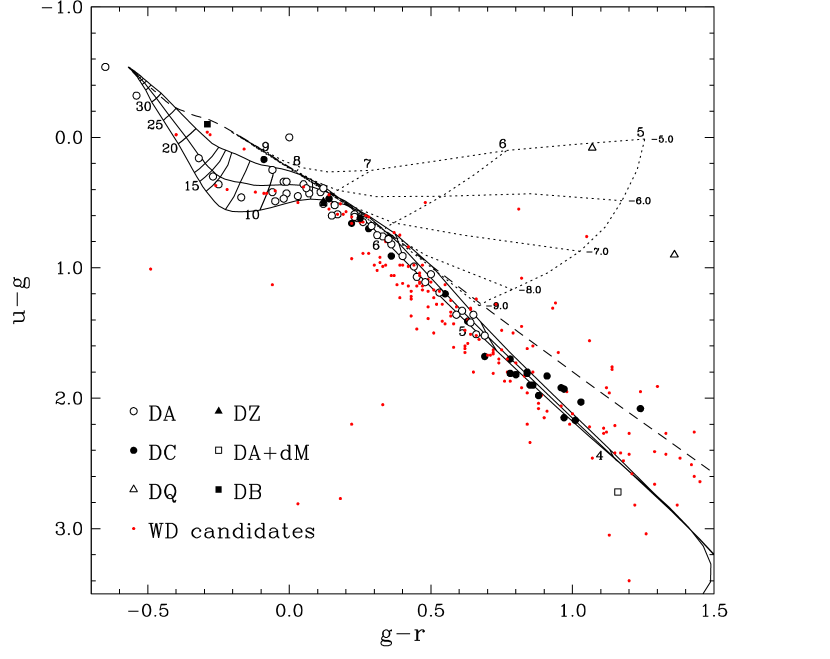
Figure 10.— ($u-g$, $g-r$) color-color diagram showing the 268 white dwarf candidates with $ugriz$ photometry available. The 76 white dwarfs spectroscopically confirmed in Section 5 are shown with various symbols explained in the legend, while those without spectroscopic data are shown with red dots. The solid curves represent pure hydrogen model atmospheres at $\log g=7.0$, 8.0, and 9.0 (from bottom to top); effective temperatures are indicated in units of $10^{3}$ K. The dashed curve corresponds to pure helium atmospheres at $\log g=8.0$, and the dotted lines represent DQ models for 5 different compositions, from $\log\rm{C/He}=-9.0$ to $-5.0$.

The 268 white dwarf candidates with available SDSS photometry are shown in Figure 10 in a ($u-g$, $g-r$) color-color diagram, together with theoretical predictions for our pure hydrogen, pure helium, and DQ models. This two-color diagram reveals that our sample is dominated by cool white dwarfs. We also expect that an important fraction of these cool objects will have a hydrogen-dominated atmosphere, and that some candidates are most likely DQ stars.

Figure 11.— Upper panel: Equal cylindrical projection of the equatorial coordinates for the sample of 1341 white dwarf candidates identified from SUPERBLINK (solid circles) compared with the sample of 499 stars from the WD Catalog recovered by our selection criteria (open circles). Also shown by the bold solid line is the region of the galactic plane. Lower panel: Space density as a function of right ascension, normalized to the total number of stars in each bin (both lines are thus on a comparable scale). The solid line represents the 1341 white dwarf candidates, while the dashed line corresponds to the white dwarfs from the WD Catalog.

The 1341 white dwarf candidates identified in SUPERBLINK are also displayed in Figure 11. The upper panel shows their space distribution using a cylindrical equal-area projection of the equatorial coordinates, while in the lower panel, the same distribution is binned into a histogram to illustrate more clearly the space density as a function of right ascension. This figure shows that our white dwarf candidates are distributed uniformly on the sky, without any drop in surface density near the galactic plane. The spectroscopically confirmed white dwarfs from the WD Catalog are also shown for comparison. Given this characteristic of our survey, we hope to increase significantly the completeness of the local white dwarf sample in this region, which has often been neglected in the past due to field crowding near the Galactic plane.

V. Spectroscopic follow-up of the candidates

We provide in this section a status report of our ongoing spectroscopic survey, and present results for a first set of 422 objects from our target list, or nearly a third of our complete sample.

Table 2Spectroscopic Observing Runs

			Grating	Blaze	Coverage	Slit
Date	Telescope	Spectrograph	(l mm-1)	(Å)	(Å)	($\arcsec$)
2009 May	Steward Observatory Bok 2.3 m	B$\&$C	600	3568	3800-5600	4.5
2009 August	NOAO Mayall 4 m	RC	527	5540	3800-6800	2
2009 November	Steward Observatory Bok 2.3 m	B$\&$C	600	3568	3800-5600	4.5
2009 December	NOAO 2.1 m	Goldcam	600	4900	3800-6700	2
2010 March	NOAO Mayall 4 m	RC	316	4000	3900-6700	2
2010 May	NOAO 2.1 m	Goldcam	500	5500	3800-6700	2
2010 July	Steward Observatory Bok 2.3 m	B$\&$C	400	4800	3800-6700	4.5
2010 October	NOAO Mayall 4 m	RC	316	5500	3900-6700	2

V.1. Spectroscopic Observations

Optical spectra have been obtained with the Steward Observatory 2.3-m telescope, and the NOAO Mayall 4-m and 2.1-m telescopes, during 8 different observing runs between 2009 May and 2010 October. The adopted configurations allow a spectral coverage of $\lambda\lambda$3200–5300 and $\lambda\lambda$3800–6700, at an intermediate resolution of $\sim 6$ Å FWHM. Spectra were first obtained at low signal-to-noise ratio (S/N $\sim 25$), which is sufficient to identify main sequence objects, but also represents the lower limit required to obtain reliable model fits to the spectral lines. Table 2 summarizes our spectroscopic observing runs and observational setups.

As a result of our spectroscopic observations, 193 newly identified white dwarfs have been spectroscopically confirmed. Among these, 68 were identified on the basis of SDSS photometry, 18 from GALEX, 70 from 2MASS, and 12 from USNO photographic magnitudes. The remaining 25 objects were discovered using an earlier version of our selection method, based on criteria different from those adopted in the final version. These objects have revised photometric distance estimates beyond 55 pc, and are thus not included in our final list of 1341 candidates.

V.2. Spectroscopic Content

Our spectroscopic follow-up observations identify 193 new white dwarfs, listed in Tables 3 and 4. Table 3 provides astrometric data as well as NLTT and SDSS designations, when available, while Table 4 lists the same objects but with the available photometry and adopted spectral types. In the earlier presentation of our results (Limoges et al., 2010), the ‘LSPM J’ notation was used for the object names, as in Lépine & Shara (2005), but the the proper motion limit for stars in SUPERBLINK has lowered to $\mu>0.04"\rm{yr}^{-1}$, and the entries were homogenized with a ‘PM I’ designation. In summary, this subsample contains 127 DA (among which 9 DA+dM and 4 magnetic), 1 DB, 56 DC, 3 DQ, and 6 DZ white dwarfs.

Once we have a confirmed white dwarf, it is possible to improve upon our preliminary distance estimates, which were based on approximate $V$ magnitudes and color-magnitude relations, by making use of the full set of photometric data. Here we rely on the so-called photometric method described at length in Giammichele et al. (2012, and references therein) where the available photometry for each star is fitted with theoretical fluxes, properly averaged over each bandpass. Both $T_{\rm eff}$ and the solid angle $\pi(R/D)^{2}$ are considered free parameters, where $R$ is the radius of the star and $D$ its distance from Earth. We assume a value of $\log g=8$ and corresponding radius $R$, and obtain directly the distance $D$. These improved photometric distances are given in Table 4.

When this survey was undertaken in 2009 May, none of these objects had a white dwarf classification or a spectral type available in the literature. But since then, white dwarf identifications have been reported in Kilic et al. (2010), Vennes et al. (2011), Tonry et al. (2012), and Sayres et al. (2012). We identified these stars in Table 3 and chose to leave these objects in our sample since they have been discovered independently. We also want to point out that even though Table 3 contains 25 stars with existing SDSS spectra, all our targets have been identified using our own spectroscopic data.

Figure 12.— (a) - Optical spectra for our sample of DA white dwarfs from SUPERBLINK. The spectra are displayed in order of decreasing equivalent width of $\rm{H}{\beta}$, from upper left to bottom right, and shifted vertically for clarity. The $\rm{H}{\alpha}$ line is also shown, when available, and normalized to a continuum set to unity.

Figure 12.— (b) - continued.

Optical spectra from our subsample of DA stars covering $\rm{H}8$ to $\rm{H}{\beta}$ — or $\rm{H}{\alpha}$ when available — are shown in Figure 12. Note that 14106+0245 (right panel of Figure 12b, second object from the top) is a DAZ, and that our subsample of 4 magnetic DA white dwarfs (05158+2839, 06019+3726, 06513+6242, and 15164+2803) are displayed in Figure 13. Our survey also detected 9 new DA white dwarfs with an M dwarf companion; these are plotted separately in Figure 14. This was quite unexpected, since the cuts in the reduced proper motion diagrams were chosen in order to avoid main sequence stars. As a consequence, we avoided all objects that are bright in the infrared portion of the spectrum. As discussed earlier, however, this is true for our criteria in $g-z$, $V-J$, and $V-I_{N}$, but not for our criteria in ${\rm{NUV}}-V$, which is efficient for detecting blue objects. And indeed, all 9 DA+dM systems were detected using this last reduced proper motion diagram.

Figure 13.— Our subsample of magnetic DA white dwarfs, shifted vertically for clarity.

Figure 14.— Our sample of binary systems composed of a DA white dwarf and a M dwarf companion. The spectra are shifted vertically for clarity. The $\rm{H}{\alpha}$ and $\rm{H}{\beta}$ line cores of 04032+2520E (not to be confused with the DA 04032+2520W), 06556+5920, 16171+0530, and 23283+3319 are contaminated by emission from the M dwarf.

The DB, DQ, and DZ stars in our sample are plotted together in Figure 15. Unfortunately, the observational setup with the NOAO telescopes does not allow the coverage of wavelengths shorter than $\sim 3900$ Å, while covering $\rm{H}{\alpha}$ simultaneously. Calcium lines can still be easily identified, however, but additional spectroscopic observations near the $\sim 3700$ Å region are currently being obtained in order to perform a proper model atmosphere analysis of these DZ stars. In the case of DQ white dwarfs, one particular object, 12476+0646, exhibits the pressure-shifted carbon lines characteristic of DQpec stars (Kowalski, 2010). Finally, we display our featureless DC spectra in Figure 16 in order of their Right Ascension.

Figure 15.— Spectra of white dwarfs in our sample with helium-rich atmospheres. The panel on the left displays the DZ stars, while the panel on the right shows our only DB star, as well as 3 DQ stars.

Figure 16.— Our sample of featureless DC stars. All spectra are normalized to a continuum set to unity and are offset from each other by a factor of 0.9.

Some of the results of our spectroscopic observations are summarized in the color-color diagram shown in Figure 10, where we identify the various spectral types of the 76 confirmed white dwarfs with available SDSS colors. As expected, the DQ stars are located in the appropriate region of the ($u-g$, $g-r$) diagram, and in the next phase of the survey, we plan to use this characteristic to identify all possible DQ stars in SUPERBLINK. We also note the presence of a DA + dM system at $(u-g,g-r)\sim(2.8,1.2)$, in the redder part of the diagram. Finally, the sample of DC stars follows the theoretical, pure hydrogen sequence, with only one outlier near $u-g=2.0$, giving us a preliminary indication of the atmospheric composition even before performing a full analysis of their energy distribution.

In the following section, we present a preliminary spectroscopic analysis of the DA component of our survey.

VI. Atmospheric Parameter Determination of DA Stars

The coolest white dwarfs in our sample are either featureless, or present too few spectral lines for a proper spectroscopic analysis, and the determination of their atmospheric parameters ($T_{\rm eff}$, $\log g$) can only be achieved from an analysis of their photometric energy distribution (see, e.g., Bergeron et al. 1997). At the moment, not enough photometric information is available to proceed with a homogeneous analysis of the coolest objects in our sample, and we are still securing the appropriate optical and infrared photometry for cool DA, DC, DQ, and DZ stars, the results of which will be reported in subsequent papers. We thus restrict our determination of the atmospheric parameters to the subsample of 84 spectroscopically confirmed DA stars for which the spectroscopic technique can be successfully applied.

VI.1. Theoretical Framework

Our model atmospheres and synthetic spectra for DA stars are built from the model atmosphere code originally described in Bergeron et al. (1995) and references therein, with recent improvements discussed in Tremblay & Bergeron (2009). These are pure hydrogen, plane-parallel model atmospheres, with non-local thermodynamic equilibrium effects explicitly taken into account above $T_{\rm eff}=30,000$ K, and energy transport by convection is included in cooler models following the ML2/$\alpha=0.7$ prescription of the mixing-length theory. The theoretical spectra are calculated within the occupation formalism of Hummer & Mihalas (1988), which provides a detailed treatment of the level populations as well as a consistent description of bound-bound and bound-free opacities. We also rely on the improved calculations for the Stark broadening of hydrogen lines from Tremblay & Bergeron (2009), which include nonideal perturbations from protons and electrons directly inside the line profile calculations. Our model grid covers a range of effective temperature between $T_{\rm eff}=1500$ K and 120,000 K, and $\log g$ values between 6.0 and 9.5.

Our fitting technique is based on the approach pioneered by Bergeron et al. (1992, see also ), which relies on the nonlinear least-squares method of Levenberg-Marquardt (Press et al., 1986). The optical spectrum of each star, as well as the model spectra (convolved with a Gaussian instrumental profile), are first normalized to a continuum set to unity. The calculation of $\chi^{2}$ is then carried out in terms of these normalized line profiles only. The atmospheric parameters – $T_{\rm eff}$, $\log g$ – are considered free parameters in the fitting procedure.

Special care needs to be taken in the case of DA stars with an unresolved M dwarf companion in order to reduce the contamination of the white dwarf spectrum by the companion. When the contamination affects only $\rm{H}{\beta}$, and sometimes $\rm{H}{\gamma}$ as well, we simply exclude these lines from the fit (e.g., 05280+4820 and 23229+3358). At other times, emission lines from the M dwarf are also observed in the center of the Balmer lines, in which case the line centers are also simply excluded from our fitting procedure (e.g., 04586+6209). A similar approach was also adopted if the flux contribution from the M dwarf is too important and “fills up” the Balmer line cores, resulting in predicted lines that are too deep (06556+5920, 16171+0530, and 23283+3319). In some cases, however, the white dwarf spectrum is too contaminated by the M dwarf companion to be fitted with the simple approach described above (e.g., 04032+2325E — not to be confused with the DA star 04032+2325W — and 11036+1555), and a more robust fitting procedure using M dwarf templates will be required (Gianninas et al., 2011). These results will be presented elsewhere.

VI.2. Spectroscopic Results

Even though the spectroscopic technique is arguably the most accurate method for measuring the atmospheric parameters of DA stars, it has an important drawback at low effective temperatures ($T_{\rm eff}\lesssim 13,000$ K) where spectroscopic values of $\log g$ are significantly larger than those of hotter DA stars, the so-called high-$\log g$ problem (see Tremblay et al. 2010 and references therein). Tremblay et al. (2011b) showed that this high-$\log g$ problem is actually related to the limitations of the mixing-length theory used to describe the convective energy transport in DA stars, and that more realistic, 3D hydrodynamical model atmospheres are required in order to obtain a surface gravity distribution that resembles that of hotter radiative-atmosphere DA stars. Since these spurious high-$\log g$ values affect directly the estimated distances, Giammichele et al. (2012) derived an empirical procedure (see their Section 5 and Figure 16) to correct the $\log g$ values based on the DA stars in the Data Release 4 of the Sloan Digital Sky Survey, analyzed by Tremblay et al. (2011a). We adopt a similar approach here and apply their $\log g$ correction to all DA stars between $T_{\rm eff}=7000$ K and 14,000 K.

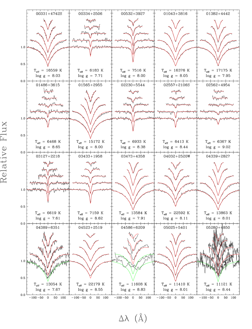
Figure 17.— (a) - Fits to the optical spectra of the DA stars in our sample. The lines range from $\rm{H}\beta$ (bottom) to H8 (top), each offset vertically by a factor of 0.2. Theoretical line profiles shown in green are not used in the fitting procedure.

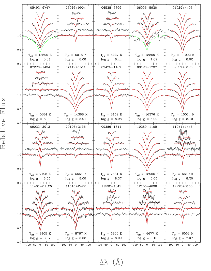
Figure 17.— (b) -continued.

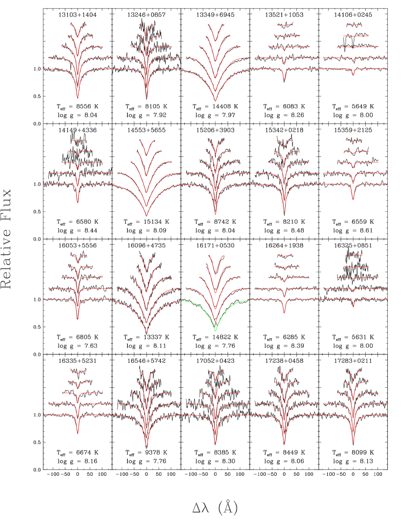
Figure 17.— (c) - continued

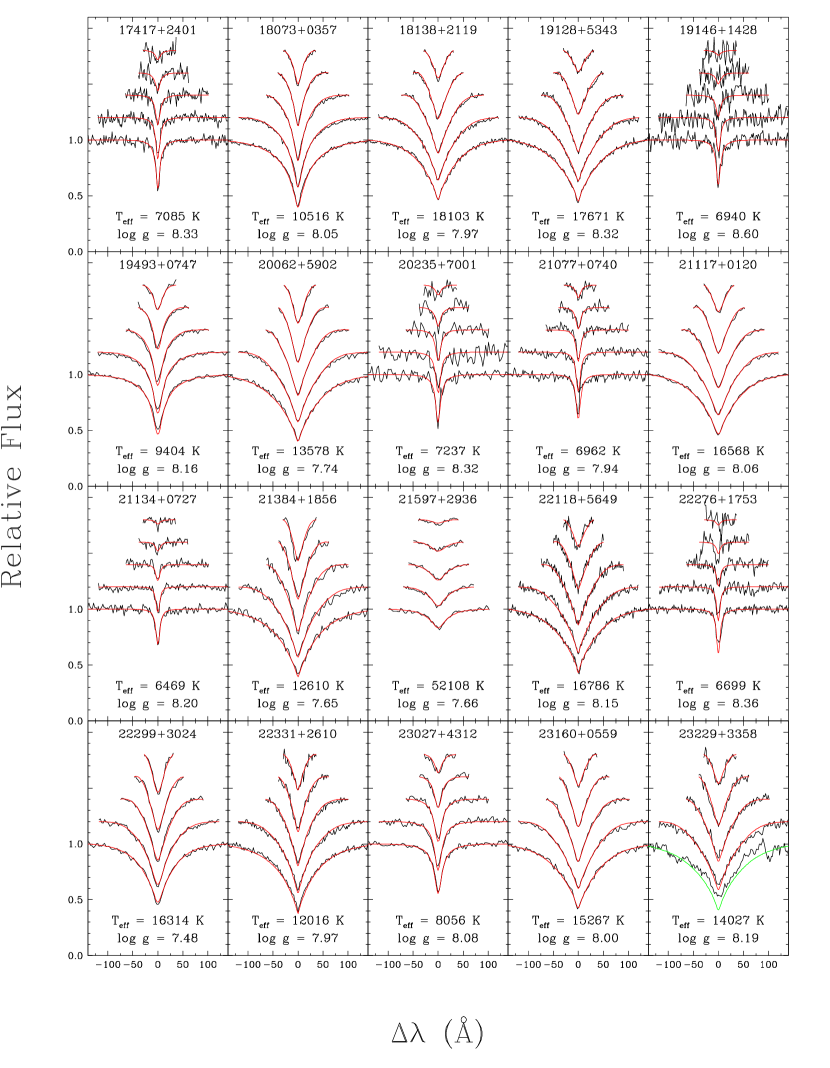
Figure 17.— (d) - continued

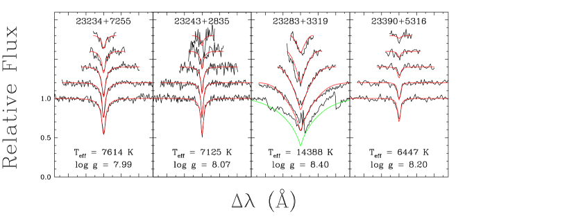
Figure 17.— (e) - continued

The spectroscopic fits for our subsample of 84 DA stars are displayed in Figure 17. The corresponding atmospheric parameters ($T_{\rm eff}$ and $\log g$) are reported in Table 5 together with the stellar mass ($M/$$M_{\odot}$), absolute absolute visual magnitude ($M_{V}$), luminosity ($L/L_{\odot}$), estimated visual magnitude ($V$), spectroscopic distance ($D$), and white dwarf cooling time ($\tau$). Whenever necessary, we rely on the same evolutionary models as those described above to derive these quantities. In principle, the spectroscopic distance can be obtained directly from the distance modulus, by combining the theoretical absolute magnitude in a single given bandpass with the observed magnitude in the same bandpass. However, since the photometric errors can be large in some systems we used — the USNO photographic magnitudes in particular —, we estimated the spectroscopic distances by using the full set of photometry available for each star, and calculated an average spectroscopic distance, properly weighted by the photometric uncertainties in each bandpass. This is equivalent to using the photometric method described above but by forcing the effective temperature at the spectroscopic value, thus fitting only the solid angle $\pi(R/D)^{2}$, where $R$ is the radius of the star determined from the spectroscopic $\log g$ value. In doing so, we also fold in the uncertainty of the spectroscopic $\log g$ measurement.

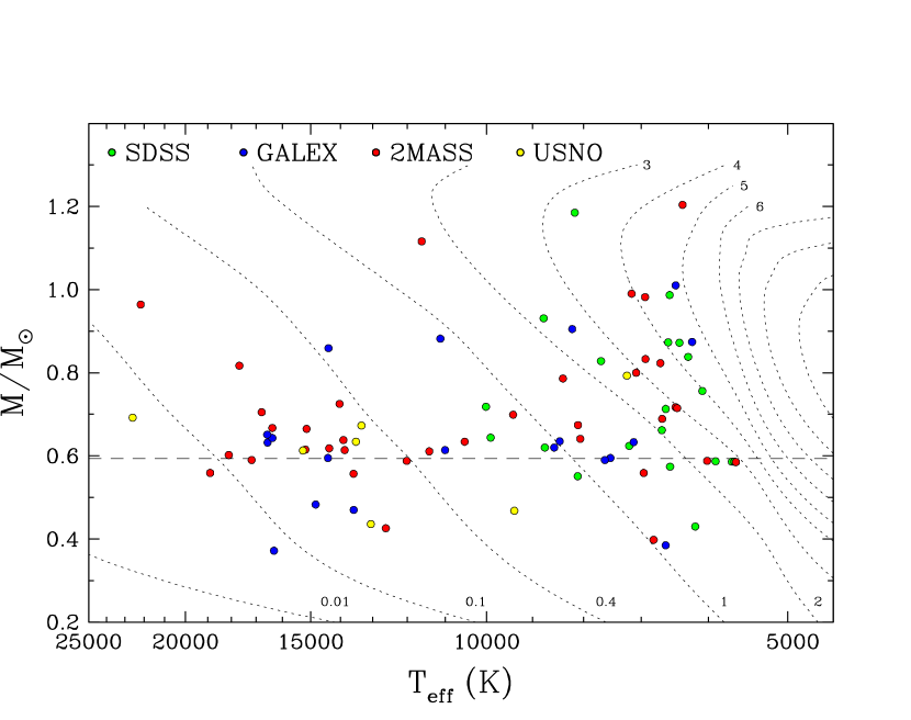
Figure 18.— Mass as a function of effective temperature for a subsample of 84 DA white dwarfs with spectroscopic mass determinations. All stars are identified with a different color based on the photometric system from which they were discovered. The dotted lines represent the theoretical isochrones for our C/O core evolutionary models with thick hydrogen layers, corresponding to the white dwarf cooling age in units of Gyr. The dashed line indicates the median mass of DA white dwarfs, 0.594 $M_{\odot}$, as determined by Tremblay et al. (2011a).

The mass distribution for the DA stars in our sample is displayed in Figure 18 as a function of effective temperature. This figure clearly illustrates the efficiency of our survey to identify white dwarfs using reduced proper motion diagrams even at very low effective temperatures. We also distinguish with various color codes the criteria used in our survey to discover each white dwarf, allowing us to study the impact of one particular photometric system on the selection process as a function of temperature. For instance, white dwarfs identified on the basis of GALEX photometry extend down to relatively low effective temperatures. Indeed, the observed photometric sequence allows us to apply our selection criteria down to ${\rm NUV}-V=6.5$ (see Figure 6), or $T_{\rm eff}\sim 5300$ K. Similarly, white dwarfs identified on the basis of $ugriz$ photometry are mostly found at the low end of the temperature distribution. Most SDSS targets are intrinsically faint, and thus include an impressive amount of cool white dwarfs that can only only be identified through the use of reduced proper motion diagrams. Surprisingly, white dwarfs identified on the basis of 2MASS photometry are found at all temperatures. This is due to the fact that our photometric sequences allow us to apply our color criteria as blue as $V-J=-0.5$ (see Figure 7), or $T_{\rm eff}\sim 20,000$ K. Finally, only a few white dwarfs in this subsample were identified on the basis of USNO photographic magnitudes. From these results, we can conclude that even though SDSS represents the most reliable photometric data set, GALEX, 2MASS, and even photometric magnitudes are also required to identify white dwarfs over the complete range of effective temperature.

Figure 19.— Mass distribution for the DA white dwarfs in our sample. The solid line histogram shows the distribution for the 84 DA stars with spectroscopic masses available, while the shaded histogram corresponds to the subsample of 37 objects with spectroscopic distances less than 40 pc from the Sun. The mean values and standard deviations are given in the figure.

The mass distribution of DA white dwarfs in our subsample, regardless of their temperature, is displayed in Figure 19. The mean mass of these 84 DA stars is 0.689 $M_{\odot}$ with a standard deviation of $\sigma=0.172$ $M_{\odot}$, a value significantly larger than the value obtained by Giammichele et al. (2012) for the DA white dwarfs within 20 pc of the Sun (0.647 $M_{\odot}$  with $\sigma=0.171$ $M_{\odot}$). One obvious difference is that we do not include here the white dwarfs already known in the literature. Most likely these are brighter, intrinsically more luminous, and probably have larger radii and thus lower masses. The mass distribution of the 37 DA white dwarfs within 40 pc of the Sun displayed in Figure 19 (shaded histogram) actually shows an important high-mass component (see also Figure 18). These high-mass white dwarfs, with their small stellar radii, are intrinsically less luminous than their normal-mass counterparts, and they are thus more abundant in a volume-limited sample, such as the local neighborhood, than in a magnitude-limited sample. Our results indicate that we are successfully recovering these high-mass white dwarfs in our survey, often missing in magnitude-limited surveys (see, e.g., Liebert et al. 2005 in the case of the PG survey).

VII. Discussion

VII.1. Comparison of Spectroscopic and Photometric Distances

During the target selection process, distances were estimated using approximate $V$ magnitudes together with various color-magnitude relations, displayed in Figures 5 to 8. These distance estimates were later improved by comparing theoretical average fluxes to the set of available photometry, properly weighted by their uncertainty. At that point, we simply assumed a surface gravity of $\log g=8.0$, and considered both $T_{\rm eff}$ and the solid angle as free parameters. These estimates are referred to as photometric distances. The spectroscopic analysis, on the other hand, provides spectroscopic distances, where for a given star, theoretical absolute magnitudes are computed from the spectroscopic values of $T_{\rm eff}$ and $\log g$, and compared to the set of available photometry. In both cases, if only the $V$ photographic magnitude is available, the 0.5 magnitude error will introduce a 23% uncertainty on the estimated spectroscopic distance. If additional photometry is available, however, this distance uncertainty can be significantly reduced (see Table 5).

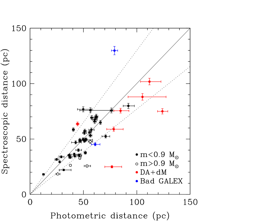
Figure 20.— Comparison of photometric and spectroscopic distances for white dwarfs with $T_{\rm eff}>7000$ K, as defined in the text. The solid line represents the 1:1 correspondence, while the dotted lines represent a $\pm 23\%$ dispersion.

The comparison between photometric and spectroscopic distances for the DA white dwarfs in our sample is displayed in Figure 20. We restrict this comparison to $T_{\rm eff}>7000$ K since the Balmer lines in cooler objects become too weak to be fitted properly with the spectroscopic method, yielding spurious $\log g$ values at low temperatures (see Figure 18) and corresponding distances. The dotted lines in Figure 20 represent a $\pm 23\%$ difference between both estimates (i.e., the maximum error on spectroscopic distances obtained from photographic magnitudes, as discussed in the previous paragraph). The bulk of stars is generally found within these limits. Part of the observed dispersion in Figure 20 can be attributed to the intrinsic mass distribution of our sample. Indeed, all our color-magnitude calibrations assumed a typical mass of 0.6 $M_{\odot}$, but as shown in Figures 5 to 8, there is an intrinsic dispersion in absolute magnitude due to the mass (or radius) distribution of white dwarfs. In particular, white dwarfs with very high ($M>0.9$ $M_{\odot}$) spectroscopic masses yield photometric distances that are overestimated; these are identified with a different symbol in Figure 20.

Another source of scatter is due to the presence of M dwarf companions, which make the system brighter at visual and infrared magnitudes compared with single DA stars. Since these magnitudes were used to estimate their photometric distance ($M_{V}$ vs $V-J$), this can easily account for the large discrepancies with spectroscopic distances. Indeed, in the spectroscopic distance calculation, the less accurate magnitudes weigh less, and the more accurate $JHK$ photometry dominates the distance solution. Finally, as noted in Table 5, we have certain doubts about the cross-correlation with the GALEX database for a handful of stars in our sample. For these objects, the GALEX photometry is inconsistent with the rest of the spectral energy distribution, and they had to be omitted from the fits used to estimate the spectroscopic distances. However, as in the previous cases, these colors were used to obtain our initial distance estimate.

To summarize, most objects in Figure 20 are found between the $\pm 23\%$ dispersion in distance, and the stars falling outside these limits can be separated into three categories: DA stars with M dwarf companions, high-mass white dwarfs, and stars with large photometric uncertainties (see the corresponding error bars in Figure 20). The previously estimated 15 pc error is thus enough to identify white dwarfs with reasonably accurate photometry, and we thus conclude that searching at 55 pc in order to find all white dwarfs within 40 pc is realistic, especially when photometry such as SDSS, GALEX, or 2MASS is available.

Our preliminary spectroscopic analysis of DA stars presented in Table 5 yields 11 white dwarf candidates within 25 pc of the Sun, including 5 candidates within the 20 pc sample. Incidentally, a few of these objects already have a parallax measurement available. Indeed, 21134+0727 (G25-20) has a parallax from Dahn et al. (1988), $\pi=0\farcs 0411\pm 0\farcs 0038$ yr^-1, placing it within 25 pc. Also, if 22118+5649 is a common proper motion companion to LTT 16500, as it is suspected to be (Subasavage et al. 2012, private communication), then it has a parallax of $\pi=0\farcs 02677\pm 0\farcs 00018$ yr^-1 (or $D=37.4$ pc), and thus not a member of the 20 pc sample, while still within 40 pc of the Sun. Finally, a private communication from J. Subasavage confirms that 16325+0851 is indeed within 25 pc of the Sun. So even though spectroscopic distances are more accurate than the previous photometric estimates, the only way to confirm the membership of white dwarfs to the local sample is through trigonometric parallax measurements. Such measurements would not only provide reliable distances, but would also yield mass determinations for the coolest objects in our sample analyzed with the photometric technique.

VII.2. Success Rate of Discovery

Figure 21.— Absolute magnitude as a function of photometric distance. In the upper panel, the filled circles represent the 193 new white dwarfs identified in our survey, while the open circles correspond to the 499 white dwarfs already known in the literature. Also shown by dashed lines in the figure are lines of constant apparent $V$ magnitudes. The white dwarf candidates in our survey without spectroscopic confirmation are shown in the lower panel. The lower-priority candidates (those identified on the basis USNO photographic magnitudes) are shown with cross symbols.

The absolute visual magnitudes (estimated from the calculated $V$ magnitudes and photometric distances) for the 193 new white dwarfs identified in our survey are plotted in the upper panel of Figure 21 as a function of photometric distance. Also shown are the 499 white dwarfs in SUPERBLINK already known in the literature. The candidates still without spectroscopic confirmation are displayed separately in the lower panel; the objects selected on the basis of their USNO photographic magnitudes are considered second priority targets because of their higher probability of being contaminants from the main sequence. In each panel, the dashed lines represent lines of constant apparent $V$ magnitude. We note that the white dwarfs identified in our survey are dominated by objects fainter than $V=16$, and that most of them are found at photometric distances larger than 20 pc. This is not surprising since the census of white dwarfs within 20 pc of the Sun is believed to be at least $90\%$ complete (Giammichele et al., 2012). There are still a few white dwarf candidates on our target list within 20 pc that have no spectroscopic data, due to observational constraints, but these stars are currently on our high priority list.

From the results shown in the upper panel of Figure 21, we can determine that the ratio of new to known white dwarfs is $193/499\sim 39\%$. Also, out of the 286 candidates observed, 220 are confirmed white dwarfs (27 in the literature and 193 in our survey), for a success rate of $77\%$. This number is close to the $80\%$ expected from our selection criteria, and we conclude that our survey is quite efficient for recovering the missing fraction of white dwarfs in the solar neighborhood.

The lower panel of Figure 21 reveals that a significant fraction of our remaining white dwarf candidates are fainter than $V=17$ (590 objects fainter versus 329 objects brighter). The spectroscopic identification of these stars with 2 to 4-m telescopes requires integration times on the order of an hour under excellent weather conditions. The candidates deserving spectroscopic follow-up must then be carefully chosen, and our high-priority list now includes 89 of these faint candidates and 186 “bright” targets, for a total of 275 high-priority targets, excluding 120 objects we already observed after 2010 October and that are still being reduced. Future observations will be dedicated to the follow-up of these high-priority white dwarf candidates, in particular those identified on the basis of SDSS or GALEX photometry.

VII.3. Increasing the completeness of the current census

Figure 22.— Transverse velocity as a function of distance, showing the kinematic bias due to the proper motion limit of the SUPERBLINK catalog ($\mu>40$ mas $\rm{yr}^{-1}$). In the upper panel, the filled circles represent the 193 new white dwarfs identified in our survey, while the open circles correspond to the 499 white dwarfs already known in the literature. Also shown by dashed lines in the figure are lines of constant apparent proper motion (in units of arcsec yr^-1). The white dwarf candidates in our survey without spectroscopic confirmation are shown in the lower panel. The lower-priority candidates (those identified on the basis USNO photographic magnitudes) are shown with cross symbols.

We have already established the success rate of our spectroscopic survey, and we are now interested in its completeness. First of all, our white dwarf sample is directly affected by the completeness of the SUPERBLINK catalog, which is high because of its low proper motion limit ($\mu>0\farcs 04$ yr^-1) which minimizes the kinematics bias. To illustrate the effect of proper motion on kinematics, we plot in Figure 22 the transverse motions $v_{t}$ (i.e. the projected motions on the plane of the sky, where $v_{t}=4.47{\mu}d$) for all stars in our sample as a function of the photometric distance $D$, as calculated in Section 4.1. As explained in Lépine & Gaidos (2011), a star at 50 pc from the Sun with $\mu>0\farcs 04$ yr^-1 has a transverse velocity $v_{t}<9.48$ km s^-1, which will occur with a probability of about $10\%$ for stars in the solar neighborhood (see their Section 2.2 and Figure 1). Their diagram shows that operating with a proper motion limit of $\mu>0\farcs 150$ yr^-1 will only detect half of the stars at 40 pc and very few stars (only those with very large components of motion) at 100 pc. However, a sample with a proper motion limit $\mu>0\farcs 04$ yr^-1 will include $\sim 95\%$ of the stars at 40 pc and $\sim 70\%$ of the stars at 100 pc.

Hence, in terms of new white dwarf identification as a function of proper motion, we find that for $\mu>0\farcs 5$ yr^-1 (see corresponding dashed line in Figure 22), which corresponds to the limit of the LHS survey, the ratio of new to known white dwarfs is $8.8\%$, while this ratio reaches 43.5% for $0\farcs 5>\mu>0\farcs 18$ yr^-1 (where the lower proper motion limit is that of the NLTT survey), and it then drops slightly to $41.3\%$ for $0\farcs 18<\mu<0\farcs 04$ yr^-1. Our survey is thus more efficient for proper motions lower than the LHS limit, but our results also demonstrate that the sample of white dwarfs with $\mu>0\farcs 5$ yr^-1 could host up to 7 more white dwarfs. Previous searches for white dwarfs within the NLTT limit were also incomplete, since 33 of our new identifications have an NLTT designation. Note also that the NLTT and LHS appear to be $\gtrsim 80\%$ complete down to the 19th magnitude, but only in the Completed Palomar Region (CPR), i.e. for $\delta>-32.5^{\circ}$ and outside a band $\pm 10^{\circ}$ of the Galactic plane (Lépine & Shara, 2005).

Spectroscopic distances were obtained for 84 out of the 193 newly identified white dwarfs, while a preliminary photometric analysis (not presented here) of a subsample of the coolest objects was performed for another 78 white dwarfs. From this combined analysis of 162 white dwarfs, we find that 126 objects are within 55 pc of the Sun, and 93 within 40 pc. The spectroscopic analysis of 1151 DA stars by Gianninas et al. (2011) contains 223 white dwarfs from the WD Catalog located in the northern hemisphere whose spectroscopic distances are within 55 pc from the Sun, and 121 within 40 pc. Using this latter survey, our ratio of new to known white dwarfs is estimated at $56\%$ within 55 pc, and $77\%$ within 40 pc. This difference in ratio will most likely be reduced when all candidates between 40 and 55 pc are observed. It was also mentioned in Section 7.2 that the ratio of new to known white dwarfs from the literature was $39\%$, while our success rate in detecting white dwarfs (both new and known) is $77\%$. Our survey is thus efficient for recovering white dwarfs that are already found in the literature as well as new identifications.

In spite of the success of our survey, the first sample of newly identified white dwarfs presented in this paper is far from complete, but the survey has not reached its limit yet. Our analysis represents the first results of an ongoing effort, and more data are still being collected and analyzed. Moreover, SUPERBLINK is currently being cross-correlated with the SDSS DR7 and GALEX GR7, providing additional high-quality photometric information to replace USNO magnitudes in our selection process. This will eventually result in more high-priority candidates, and will also help in the identification of DQ and DZ stars, which separate well in color-color diagrams, as we showed earlier, but only when such color information is available. Finally, these new magnitudes may also complete the set of photometry for white dwarfs in the SUPERBLINK catalog, allowing fits to the energy distribution of the cool white dwarfs that cannot be analyzed spectroscopically. Our future catalog will provide more candidates for parallax measurements, as well as more cool, massive, magnetic, and astrophysically challenging white dwarfs, while being at least $80\%$ complete within 40 pc of the Sun. We will also be able to provide statistics on the Solar Neighborhood based on a sample of white dwarfs large enough to reduce the uncertainties related to small number statistics.

Table 3Spectroscopically Confirmed White Dwarfs from SUPERBLINK $-$ Astrometry

			RA	DEC	$\mu_{\rm{tot}}$	$\mu$RA	$\mu$DE
PM I	NLTT	SDSS	($J_{2000}$)	($J_{2000}$)	$(\arcsec\rm{yr}^{-1})$	$(\arcsec\rm{yr}^{-1})$	$(\arcsec\rm{yr}^{-1})$	Notes
00023$+$6357			00:02:22.61	+63:57:44.3	0.911	0.906	0.092
00079$+$3947	317		00:07:54.11	+39:47:32.2	0.370	0.362	$-$0.075
00217$+$2640	1119		00:21:47.32	+26:40:36.3	0.330	$-$0.074	$-$0.322
00276$+$0542			00:27:36.63	+05:42:03.2	0.381	0.266	$-$0.273
00331$+$4742S			00:33:10.51	+47:42:12.4	0.079	$-$0.060	0.052
00334$+$2506	1783	J003325.44+25061	00:33:25.28	+25:06:14.1	0.499	0.477	0.146
00532$+$3927			00:53:13.75	+39:27:06.1	0.209	$-$0.152	$-$0.143
00559$+$5948			00:55:58.28	+59:48:02.4	0.458	0.454	$-$0.061
01043$+$3816			01:04:19.32	+38:16:55.0	0.070	$-$0.054	$-$0.046
01216$+$3440		J012137.74+34404	01:21:37.80	+34:40:43.2	0.132	$-$0.131	0.017
01382$+$4442			01:38:12.93	+44:42:52.2	0.049	$-$0.014	$-$0.047
01457$+$2918	5850		01:45:44.62	+29:18:23.8	0.529	0.529	0.008
01486$+$3615	6026		01:48:40.45	+36:15:31.0	0.231	0.000	$-$0.231
01565$+$2955			01:56:29.90	+29:55:35.9	0.104	0.054	$-$0.089
02062$+$1836	6996		02:06:14.67	+18:36:24.1	0.789	0.784	0.093
02118$+$7119		J021148.35+71191	02:11:48.17	+71:19:13.3	0.252	0.166	$-$0.190
02149$+$7746			02:14:56.99	+77:46:00.0	0.469	0.265	$-$0.387
02230$+$5544			02:23:00.30	+55:44:27.2	0.172	0.126	$-$0.117
02237$+$2055		J022348.96+20555	02:23:48.93	+20:55:53.8	0.477	0.014	$-$0.476
02334$+$2125		J023339.00+21251	02:33:38.98	+21:25:13.2	0.234	0.062	$-$0.226
02379$+$1638	8525		02:37:59.15	+16:38:13.0	0.321	$-$0.036	$-$0.319
02478$+$4138			02:47:51.80	+41:38:29.6	0.074	$-$0.018	$-$0.072
02497$+$3307		J024944.28+33072	02:49:44.20	+33:07:25.6	0.303	0.175	0.247
02557$+$2106S		J025545.70+21062	02:55:45.60	+21:06:21.7	0.257	0.225	$-$0.125
02562$+$4954	9314		02:56:17.18	+49:54:41.9	0.193	0.032	$-$0.191
03109$+$6634			03:10:57.60	+66:34:02.1	0.812	0.691	$-$0.426
03127$+$2218	10206		03:12:42.85	+22:18:28.5	0.277	0.202	$-$0.189
03196$+$3630			03:19:38.25	+36:30:29.5	0.107	0.105	0.016
03203$+$2333	10606		03:20:20.30	+23:33:31.7	0.366	0.077	$-$0.358
03433$+$1958			03:43:23.11	+19:58:13.5	0.177	0.081	0.157
03473$+$4358			03:47:22.43	+43:58:57.2	0.176	$-$0.160	0.074
04010$+$5131W		J040101.58+51313	04:01:01.50	+51:31:30.2	0.890	0.365	$-$0.812
04032$+$2520E			04:03:16.51	+25:20:19.2	0.051	$-$0.045	$-$0.025
04032$+$2520W			04:03:16.51	+25:20:19.2	0.051	$-$0.045	$-$0.025
04259$+$4614			04:25:57.00	+46:14:17.6	0.174	0.157	$-$0.075
04263$+$4820			04:26:23.59	+48:20:09.7	0.128	0.039	$-$0.122
04334$+$0414			04:33:29.80	+04:14:47.7	0.463	0.092	$-$0.453
04339$+$2827			04:33:54.42	+28:27:31.1	0.060	0.047	$-$0.038
04343$+$3054			04:34:20.55	+30:54:22.4	0.307	$-$0.040	$-$0.305
04389$+$6351			04:38:56.94	+63:51:34.2	0.184	0.145	$-$0.113
04523$+$2519			04:52:19.36	+25:19:34.0	0.104	0.004	$-$0.104	1
04558$+$3840			04:55:51.38	+38:40:50.4	0.220	0.210	$-$0.069
04586$+$6209			04:58:39.26	+62:09:07.9	0.144	0.112	$-$0.092
05025$+$5401			05:02:34.18	+54:01:08.5	0.190	$-$0.040	$-$0.185
05158$+$2839			05:15:53.53	+28:39:16.6	0.200	0.160	$-$0.109
05269$+$4435			05:26:56.11	+44:35:39.1	0.450	0.250	$-$0.381
05280$+$4850			05:28:03.21	+48:50:47.5	0.130	0.029	$-$0.126
05327$+$0624			05:32:42.87	+06:24:28.6	0.066	$-$0.059	$-$0.030
05492$+$5747			05:49:14.55	+57:47:57.3	0.090	0.063	0.064
06019$+$3726			06:01:58.71	+37:26:02.1	0.074	0.009	$-$0.073
06026$+$0904			06:02:36.72	+09:04:23.6	0.268	0.098	$-$0.250
06324$+$2230			06:32:29.37	+22:30:04.6	0.210	$-$0.140	$-$0.157
06492$+$1519			06:49:17.30	+15:19:30.9	0.346	0.246	$-$0.243
06506$+$1657			06:50:36.80	+16:57:53.7	0.268	$-$0.175	$-$0.202
06513$+$6242			06:51:22.90	+62:42:54.9	0.143	$-$0.075	$-$0.122
06538$+$6355			06:53:50.41	+63:55:58.1	0.432	$-$0.142	$-$0.407
06556$+$5920			06:55:38.50	+59:20:27.4	0.150	0.000	$-$0.159
07029$+$4406			07:02:58.93	+44:06:53.8	0.093	0.092	$-$0.001
07241$+$0431			07:24:06.16	+04:31:30.2	0.417	0.076	$-$0.410
07270$+$1434	17874	J072704.21+14343	07:27:04.15	+14:34:40.3	0.192	0.150	$-$0.119
07419$+$0136			07:41:54.02	+01:36:45.0	0.267	0.143	$-$0.226
07419$+$1511		J074156.42+15111	07:41:56.44	+15:11:17.0	0.119	0.004	$-$0.119
07451$+$2627		J074509.02+26270	07:45:08.94	+26:27:06.6	0.890	0.490	$-$0.744
07475$+$1107		J074730.12+11073	07:47:30.09	+11:07:35.0	0.190	0.060	$-$0.181
08126$+$1737		J081237.82+17370	08:12:37.80	+17:37:01.4	0.114	0.077	$-$0.084	1
08152$+$1633		J081516.84+16331	08:15:16.79	+16:33:17.0	0.266	0.244	$-$0.106	2
08223$+$2023		J082219.23+20232	08:22:19.23	+20:23:26.2	0.100	0.040	$-$0.100	2
08281$+$0942		J082808.04+09421	08:28:07.93	+09:42:17.8	0.460	0.440	$-$0.142
08293$+$2539		J082922.05+25393	08:29:22.84	+25:39:39.9	0.563	0.227	$-$0.515
08516$+$1624	20389	J085140.35+16245	08:51:40.48	+16:24:54.4	0.430	$-$0.410	$-$0.156
08558$+$3700		J085549.88+37001	08:55:49.86	+37:00:16.8	0.160	0.130	$-$0.094	3
09021$+$2010		J090208.40+20104	09:02:08.31	+20:10:51.6	0.345	0.098	$-$0.330	2
09026$+$1535	20824	J090240.47+15355	09:02:40.60	+15:35:57.8	0.382	$-$0.309	$-$0.224	2
09027$+$3120		J090242.66+31204	09:02:42.67	+31:20:43.9	0.087	$-$0.087	$-$0.002
09033$+$2012	20852	J090318.54+20124	09:03:18.57	+20:12:46.7	0.204	$-$0.009	$-$0.204	2,4
09106$+$2156	21118	J091037.29+21561	09:10:37.21	+21:56:16.1	0.303	0.225	$-$0.203	4
09245$+$3120	21660	J092430.80+31203	09:24:30.85	+31:20:33.5	0.424	$-$0.193	$-$0.378	2,4
09286$+$1841	21844	J092840.28+18411	09:28:40.22	+18:41:14.9	0.295	0.165	$-$0.245	2
09432$+$5134		J094316.62+51344	09:43:16.59	+51:34:41.3	0.292	0.127	$-$0.263	3
09481$+$2023	22620	J094806.09+20231	09:48:06.15	+20:23:15.4	0.203	$-$0.202	0.019	2
09503$+$1509		J095021.77+15090	09:50:21.80	+15:09:10.1	0.323	$-$0.069	$-$0.310
10155$+$1850	23818	J101535.36+18502	10:15:35.40	+18:50:22.9	0.212	$-$0.079	$-$0.197	2
10289$+$1105		J102854.91+11055	10:28:54.88	+11:05:51.3	0.091	0.067	$-$0.062
10403$+$1004		J104019.68+10040	10:40:19.70	+10:04:00.4	0.147	$-$0.098	$-$0.110
10521$+$4050	25548	J105211.67+40500	10:52:11.73	+40:50:04.2	0.276	$-$0.200	$-$0.190
10565$+$2336	25771	J105630.01+23361	10:56:30.08	+23:36:19.0	0.282	$-$0.181	$-$0.216	4
11036$+$1555		J110338.81+15551	11:03:38.85	+15:55:14.6	0.097	$-$0.092	0.030
11071$+$1446	26335	J110709.66+14465	11:07:09.72	+14:46:54.4	0.281	$-$0.264	0.097	4
11253$+$2111	27340	J112521.29+21111	11:25:21.41	+21:11:15.2	0.398	$-$0.267	$-$0.295
11337$+$6243		J113347.79+62431	11:33:47.81	+62:43:13.3	0.122	$-$0.063	0.104
11401$+$0112W		J114009.11+01122	11:40:09.12	+01:12:23.0	0.166	$-$0.165	$-$0.014
11545$+$2422		J115434.57+24223	11:54:34.57	+24:22:39.5	0.110	0.016	$-$0.109	2,4
11582$+$0004		J115814.51+00045	11:58:14.51	+00:04:58.4	0.180	$-$0.038	0.176	3
11592$+$4842	29180	J115916.47+48423	11:59:16.51	+48:42:38.9	0.236	$-$0.226	$-$0.067
11598$+$0007		J115952.04+00075	11:59:52.03	+00:07:51.7	0.090	0.079	$-$0.044
12113$+$0724		J121118.80+07244	12:11:18.82	+07:24:48.2	0.227	$-$0.065	$-$0.218	3,4
12155$+$4630	30149	J121531.63+46301	12:15:31.71	+46:30:14.0	0.269	$-$0.269	0.016	5
12273$+$3150		J122724.30+31502	12:27:24.27	+31:50:24.0	0.204	0.084	$-$0.186	2,4
12280$+$3300		J122801.59+33003	12:28:01.57	+33:00:36.3	0.187	0.048	$-$0.181	2
12370$+$1814		J123700.74+18145	12:37:00.77	+18:14:59.1	0.229	$-$0.181	$-$0.139	2
12377$+$6023		J123743.15+60232	12:37:43.16	+60:23:20.4	0.159	$-$0.064	0.146
12405$+$1807W	31483	J124030.27+18072	12:40:30.48	+18:07:28.8	0.571	$-$0.565	$-$0.085
12425$+$1311W		J124234.43+13114	12:42:34.49	+13:11:42.1	0.343	$-$0.274	$-$0.207
12476$+$0646		J124739.04+06460	12:47:39.12	+06:46:04.3	0.389	$-$0.383	0.065	2,3
12541$+$3620	32251	J125411.37+36205	12:54:11.51	+36:20:58.4	0.407	$-$0.406	$-$0.028
13103$+$1404		J131023.76+14041	13:10:23.77	+14:04:20.5	0.134	$-$0.037	$-$0.129	2,4
13176$+$0621		J131737.45+06212	13:17:37.40	+06:21:21.5	0.304	0.262	$-$0.154	3
13246$+$0857		J132436.88+08575	13:24:36.87	+08:57:54.6	0.219	0.088	$-$0.201	2,4
13333$+$2450		J133319.26+24504	13:33:19.22	+24:50:49.6	0.209	$-$0.072	$-$0.196	2
13349$+$6945			13:34:59.90	+69:45:29.4	0.048	$-$0.019	0.044
13455$+$4200	35148	J134532.91+42004	13:45:32.97	+42:00:43.7	0.238	$-$0.203	0.123
13521$+$1053		J135211.73+10535	13:52:11.79	+10:53:51.8	0.309	$-$0.242	$-$0.192
14067$+$3130	36284	J140644.53+31302	14:06:44.61	+31:30:22.7	0.301	$-$0.214	0.212
14106$+$0245		J141039.97+02451	14:10:39.97	+02:45:13.1	0.247	$-$0.038	$-$0.244	4
14149$+$4336	36723	J141454.73+43365	14:14:54.79	+43:36:58.4	0.243	$-$0.205	$-$0.131	2
14236$+$3037		J142336.65+30374	14:23:36.64	+30:37:42.5	0.203	0.023	$-$0.201	2
14244$+$6246		J142429.52+62461	14:24:29.52	+62:46:17.0	0.272	$-$0.269	$-$0.041
14277$+$0532		J142748.11+05323	14:27:48.13	+05:32:32.5	0.250	$-$0.179	$-$0.174	2,4
14339$+$1907		J143358.19+19073	14:33:58.20	+19:07:38.3	0.210	$-$0.137	$-$0.160
14407$+$0807		J144045.12+08072	14:40:45.06	+08:07:29.3	0.294	0.229	$-$0.186
14553$+$5655		J145521.34+56554	14:55:21.35	+56:55:44.2	0.076	$-$0.075	0.015
14588$+$1146		J145848.51+11465	14:58:48.54	+11:46:56.2	0.168	$-$0.129	$-$0.107	3,4
15164$+$2803		J151625.07+28032	15:16:25.10	+28:03:22.2	0.107	$-$0.106	$-$0.010	2
15206$+$3903		J152038.34+39034	15:20:38.36	+39:03:49.3	0.169	$-$0.095	0.139
15263$+$2936		J152621.08+29362	15:26:21.06	+29:36:22.7	0.188	0.086	0.167
15342$+$0218		J153417.49+02184	15:34:17.50	+02:18:48.0	0.143	$-$0.118	$-$0.080	2,4
15359$+$2125		J153554.02+21250	15:35:54.06	+21:25:06.6	0.248	$-$0.142	0.203
15494$+$4802		J154927.19+48022	15:49:27.20	+48:02:29.0	0.176	0.108	$-$0.139	2,4
15589$+$0417		J155857.68+04170	15:58:57.69	+04:17:05.1	0.071	$-$0.025	$-$0.066	2
16053$+$5556		J160520.60+55564	16:05:20.69	+55:56:45.4	0.274	$-$0.222	0.160
16096$+$4735		J160939.78+47350	16:09:39.74	+47:35:10.7	0.062	0.043	$-$0.044
16171$+$0530		J161710.56+05303	16:17:10.56	+05:30:38.2	0.097	0.011	$-$0.096
16264$+$1938		J162626.28+19384	16:26:26.33	+19:38:39.3	0.275	$-$0.174	0.213
16325$+$0851		J163233.27+08512	16:32:33.17	+08:51:22.6	0.375	0.271	$-$0.259	4
16335$+$5231	43101	J163332.24+52314	16:33:32.14	+52:31:50.0	0.265	0.103	$-$0.244
16477$+$2636		J164744.70+26364	16:47:44.74	+26:36:46.3	0.204	$-$0.151	0.137	2
16546$+$5742			16:54:41.01	+57:42:16.3	0.066	$-$0.058	0.031
17027$+$1022		J170246.29+10224	17:02:46.29	+10:22:41.2	0.255	0.077	0.243
17052$+$0423			17:05:13.25	+04:23:45.3	0.168	0.009	$-$0.167
17238$+$0458			17:23:49.57	+04:58:49.1	0.149	$-$0.041	$-$0.143
17283$+$0211			17:28:18.47	+02:11:10.2	0.224	$-$0.029	$-$0.223
17335$+$7949			17:33:34.29	+79:49:16.3	0.397	0.394	$-$0.045
17417$+$2401			17:41:46.23	+24:01:49.6	0.360	$-$0.030	$-$0.359
17433$+$1434S			17:43:22.97	+14:34:52.4	0.386	$-$0.252	0.293
17471$+$2859			17:47:08.30	+28:59:09.8	0.198	$-$0.121	$-$0.157
18014$+$5049		J180127.50+50495	18:01:27.49	+50:49:58.2	0.288	$-$0.108	0.267
18073$+$0357			18:07:23.37	+03:57:01.7	0.121	$-$0.012	$-$0.121
18138$+$2119			18:13:48.55	+21:19:20.6	0.050	0.019	0.046
18199$+$1739			18:19:59.23	+17:39:19.0	0.230	0.216	0.080
18572$+$2026			18:57:13.95	+20:26:28.4	0.316	$-$0.013	$-$0.316
19128$+$5343			19:12:48.56	+53:43:13.5	0.205	0.148	0.142
19132$+$2949			19:13:16.53	+29:49:28.2	0.287	$-$0.056	0.281
19146$+$1428			19:14:36.11	+14:28:25.4	0.422	$-$0.114	$-$0.406
19464$+$0937			19:46:29.80	+09:37:14.9	0.574	0.060	$-$0.571
19493$+$0747			19:49:23.51	+07:47:31.7	0.184	0.137	$-$0.122
20062$+$5902		J200616.93+59022	20:06:16.96	+59:02:27.3	0.108	$-$0.019	$-$0.106
20069$+$6143		J200655.03+61430	20:06:54.89	+61:43:10.3	0.238	0.168	$-$0.168
20223$+$8333			20:22:21.50	+83:33:55.6	0.208	$-$0.127	0.166
20235$+$7001			20:23:29.87	+70:01:55.5	0.320	$-$0.260	$-$0.186
20597$+$5517		J205945.11+55173	20:59:44.91	+55:17:29.9	0.498	0.274	0.417
21077$+$0740			21:07:45.05	+07:40:44.3	0.116	$-$0.019	$-$0.114
21117$+$0120			21:11:46.37	+01:20:54.4	0.068	0.058	$-$0.035
21134$+$0727			21:13:28.92	+07:27:04.2	0.341	0.321	0.115
21222$+$0413		J212212.31+04135	21:22:12.35	+04:13:56.7	0.425	$-$0.089	$-$0.415	4
21384$+$1856		J213827.28+18564	21:38:27.28	+18:56:41.9	0.169	$-$0.141	$-$0.093
21420$+$2252			21:42:03.90	+22:52:29.0	0.186	0.118	$-$0.144
21429$+$0805			21:42:54.49	+08:05:27.4	0.218	$-$0.098	$-$0.195
21492$+$0415			21:49:13.60	+04:15:50.2	0.227	0.011	$-$0.226
21551$+$4103			21:55:06.36	+41:03:06.6	0.193	0.172	0.087
21597$+$2936			21:59:46.94	+29:36:41.7	0.097	0.097	0.005	1
22105$+$4532			22:10:34.53	+45:32:40.0	0.361	$-$0.122	$-$0.340
22118$+$5649			22:11:53.64	+56:49:46.4	0.250	0.249	0.022
22276$+$1753	53908		22:27:40.36	+17:53:21.4	0.219	0.203	$-$0.081
22299$+$3024			22:29:58.03	+30:24:10.6	0.122	0.050	$-$0.111
22331$+$2610			22:33:11.59	+26:10:14.9	0.089	0.085	0.026
22418$+$0432			22:41:53.18	+04:33:00.2	0.226	0.115	$-$0.194
22447$+$1513W			22:44:43.02	+15:13:46.3	0.291	0.162	0.241
22497$+$3623	54984		22:49:46.43	+36:23:22.8	0.370	0.330	$-$0.167
22595$+$5717			22:59:33.81	+57:17:57.3	0.334	$-$0.316	$-$0.109
23003$+$2204			23:00:21.96	+22:04:16.0	0.225	0.201	0.102
23027$+$4312			23:02:44.89	+43:12:47.7	0.181	$-$0.174	$-$0.051
23056$+$4334			23:05:39.06	+43:34:03.8	0.270	$-$0.120	$-$0.230
23098$+$5506E			23:09:58.53	+55:06:49.1	0.408	0.406	0.040
23160$+$0559		J231605.60+05594	23:16:05.46	+05:59:46.6	0.178	0.175	0.034
23229$+$3358			23:22:59.82	+33:58:47.1	0.179	0.128	0.125
23234$+$7255			23:23:28.24	+72:55:07.4	0.088	0.069	0.055
23243$+$2835			23:24:18.85	+28:35:55.5	0.134	$-$0.050	$-$0.124
23283$+$3319			23:28:18.03	+33:19:31.1	0.147	0.053	$-$0.137
23389$+$2101E			23:38:56.29	+21:01:18.2	0.338	0.290	0.174
23390$+$5316			23:39:00.48	+53:16:00.0	0.467	0.466	0.033
23462$+$1158			23:46:12.50	+11:58:49.7	0.136	$-$0.107	$-$0.084
23475$+$0304		J234735.20+03043	23:47:35.11	+03:04:31.9	0.278	0.177	0.215
23478$+$0223		J234753.64+02234	23:47:53.76	+02:23:40.8	0.224	$-$0.183	$-$0.129

Note. — (1) Also in Vennes et al. (2011); (2) Classified using our own data, but SDSS spectrum exists; (3) Also in Kilic et al. (2010); (4) Also in Sayres et al. (2012); (5) Also in Tonry et al. (2012).

Table 4Spectroscopically Confirmed White Dwarfs from SUPERBLINK $-$ Photometry

PM I	FUV	NUV	$B_{F}$	$R_{I}$	$I_{N}$	$J$	$H$	$K_{S}$	$u$	$g$	$r$	$i$	$z$	$\rm{D_{phot}}$ (pc)	ST	Notes
00023$+$6357	$-$	$-$	$-$	16.2	17.3	15.80	15.57	15.51	$-$	$-$	$-$	$-$	$-$	25.9	DC
00079$+$3947	$-$	$-$	17.4	16.2	15.8	15.18	14.85	14.65	$-$	$-$	$-$	$-$	$-$	20.2	DC
00217$+$2640	$-$	$-$	17.9	17.2	16.9	16.18	15.91	15.81	$-$	$-$	$-$	$-$	$-$	35.2	DC
00276$+$0542	$-$	$-$	17.2	15.6	15.4	14.97	14.67	14.57	$-$	$-$	$-$	$-$	$-$	18.2	DA
00331$+$4742S	14.55	14.63	14.9	14.9	$-$	15.16	15.02	15.14	$-$	$-$	$-$	$-$	$-$	50.8	DA
00334$+$2506	$-$	20.36	16.6	16.6	16.1	15.96	15.70	15.45	17.88	17.12	16.79	16.69	16.68	37.0	DA
00532$+$3927	$-$	18.45	17.9	16.4	16.8	16.03	15.84	15.40	$-$	$-$	$-$	$-$	$-$	54.4	DA
00559$+$5948	$-$	$-$	15.2	16.0	15.8	15.44	15.21	15.03	$-$	$-$	$-$	$-$	$-$	32.1	DC:
01043$+$3816	14.70	14.80	15.6	15.4	$-$	15.29	15.32	15.14	$-$	$-$	$-$	$-$	$-$	55.7	DA
01216$+$3440	$-$	19.61	17.9	16.3	15.9	16.13	16.15	15.88	17.27	16.76	16.64	16.64	16.74	43.6	DZ
01382$+$4442	$-$	$-$	15.5	16.0	15.2	15.62	15.61	15.71	$-$	$-$	$-$	$-$	$-$	60.5	DA
01457$+$2918	$-$	$-$	18.4	18.0	17.7	16.56	16.09	15.51	$-$	$-$	$-$	$-$	$-$	31.1	DC
01486$+$3615	$-$	20.64	17.6	16.5	16.3	15.85	15.48	15.42	$-$	$-$	$-$	$-$	$-$	37.0	DA
01565$+$2955	14.56	14.68	14.7	14.9	$-$	14.96	15.04	15.18	$-$	$-$	$-$	$-$	$-$	46.8	DA
02062$+$1836	$-$	$-$	19.2	17.8	17.1	16.50	16.38	15.63	$-$	$-$	$-$	$-$	$-$	31.0	DC:
02118$+$7119	$-$	$-$	17.8	16.4	16.6	15.78	15.42	15.32	19.04	17.57	16.94	16.67	16.57	28.1	DC
02149$+$7746	$-$	$-$	19.2	18.0	18.1	16.48	17.50	15.89	$-$	$-$	$-$	$-$	$-$	67.9	DC:	1
02230$+$5544	$-$	$-$	17.2	16.6	16.8	16.07	15.77	15.68	$-$	$-$	$-$	$-$	$-$	39.6	DA
02237$+$2055	$-$	$-$	17.0	14.9	$-$	12.28	11.65	11.45	19.26	16.60	15.17	14.12	13.56	58.6	DC
02334$+$2125	$-$	$-$	18.4	16.5	$-$	14.32	13.63	13.44	21.11	18.53	16.99	16.11	15.61	25.9	DC
02379$+$1638	$-$	$-$	17.6	16.8	16.7	15.97	15.83	14.88	$-$	$-$	$-$	$-$	$-$	24.3	DC
02478$+$4138	16.81	16.41	15.1	16.3	16.4	16.95	17.86	17.19	$-$	$-$	$-$	$-$	$-$	79.7	DB
02497$+$3307	$-$	$-$	18.0	16.7	16.4	16.01	15.49	15.39	18.48	17.43	16.97	16.79	16.73	34.9	DA
02557$+$2106S	$-$	$-$	17.7	17.1	16.5	16.48	16.04	16.06	18.47	17.68	17.36	17.25	17.20	41.3	DA
02562$+$4954	$-$	$-$	17.5	17.1	16.4	16.17	15.79	15.45	$-$	$-$	$-$	$-$	$-$	30.1	DA
03109$+$6634	$-$	$-$	18.8	17.7	17.4	16.55	16.30	15.31	$-$	$-$	$-$	$-$	$-$	29.4	DC
03127$+$2218	$-$	19.86	17.8	16.4	16.8	16.13	15.85	15.88	$-$	$-$	$-$	$-$	$-$	46.8	DA
03196$+$3630	$-$	20.96	17.3	16.2	16.1	15.84	15.84	15.38	$-$	$-$	$-$	$-$	$-$	36.7	DZ
03203$+$2333	$-$	$-$	18.9	17.0	17.0	16.21	15.65	15.76	$-$	$-$	$-$	$-$	$-$	29.2	DC
03433$+$1958	$-$	$-$	16.6	15.2	15.2	14.95	14.96	15.04	$-$	$-$	$-$	$-$	$-$	27.6	DA
03473$+$4358	$-$	$-$	14.3	14.3	14.3	14.23	14.30	14.36	$-$	$-$	$-$	$-$	$-$	29.9	DA
04010$+$5131W	$-$	$-$	17.5	16.8	16.4	15.93	15.74	15.20	19.33	17.78	17.08	16.83	16.72	141.5	DC
04032$+$2520E	$-$	$-$	15.4	14.6	13.0	12.36	11.77	11.51	$-$	$-$	$-$	$-$	$-$	112.8	DA+dM
04032$+$2520W	$-$	$-$	15.4	14.6	13.0	12.36	11.77	11.51	$-$	$-$	$-$	$-$	$-$	112.8	DA
04259$+$4614	$-$	$-$	19.0	17.2	17.0	16.46	16.00	16.08	$-$	$-$	$-$	$-$	$-$	32.4	DC
04263$+$4820	16.92	16.97	16.0	15.9	15.9	15.64	15.65	15.30	$-$	$-$	$-$	$-$	$-$	44.6	DA	2
04334$+$0414	$-$	$-$	17.4	16.3	16.1	15.55	15.26	15.18	$-$	$-$	$-$	$-$	$-$	27.5	DA
04339$+$2827	$-$	$-$	16.0	15.8	$-$	15.48	14.79	14.56	$-$	$-$	$-$	$-$	$-$	56.5	DA
04343$+$3054	$-$	$-$	18.8	17.6	17.5	16.49	16.35	15.83	$-$	$-$	$-$	$-$	$-$	36.3	DC:
04389$+$6351	$-$	$-$	17.2	16.8	16.1	15.39	14.72	14.24	$-$	$-$	$-$	$-$	$-$	39.5	DA
04523$+$2519	$-$	$-$	15.2	14.8	14.6	15.08	15.15	15.17	$-$	$-$	$-$	$-$	$-$	55.8	DA	3
04558$+$3840	$-$	$-$	18.1	16.9	16.8	16.14	15.85	15.32	$-$	$-$	$-$	$-$	$-$	32.5	DA
04586$+$6209	$-$	$-$	15.5	14.1	$-$	11.31	10.76	10.55	$-$	$-$	$-$	$-$	$-$	78.7	DA+dM
05025$+$5401	$-$	$-$	15.3	15.4	15.3	15.27	15.30	15.08	$-$	$-$	$-$	$-$	$-$	42.3	DA
05158$+$2839	$-$	19.58	16.5	16.0	15.9	15.66	15.31	15.27	$-$	$-$	$-$	$-$	$-$	35.2	DAH
05269$+$4435	$-$	$-$	18.8	17.4	17.5	16.50	16.42	15.85	$-$	$-$	$-$	$-$	$-$	36.7	DC
05280$+$4850	18.18	17.53	17.2	15.0	13.1	12.60	12.00	11.73	$-$	$-$	$-$	$-$	$-$	124.2	DA+dM
05327$+$0624	$-$	$-$	16.5	16.1	16.1	$-$	$-$	$-$	$-$	$-$	$-$	$-$	$-$	59.5	DA	4
05492$+$5747	$-$	$-$	15.8	14.7	13.6	12.76	12.21	12.00	$-$	$-$	$-$	$-$	$-$	86.9	DA+dM
06019$+$3726	$-$	$-$	16.4	17.0	16.3	$-$	$-$	$-$	$-$	$-$	$-$	$-$	$-$	35.5	DAH
06026$+$0904	$-$	$-$	17.4	16.5	16.0	15.95	15.54	15.25	$-$	$-$	$-$	$-$	$-$	27.9	DA
06324$+$2230	$-$	$-$	$-$	17.1	16.5	16.12	15.81	15.76	$-$	$-$	$-$	$-$	$-$	35.5	DA
06492$+$1519	$-$	$-$	18.1	17.3	16.6	$-$	$-$	$-$	$-$	$-$	$-$	$-$	$-$	35.8	DC
06506$+$1657	$-$	$-$	17.9	16.9	16.6	16.14	15.73	15.31	$-$	$-$	$-$	$-$	$-$	32.7	DA
06513$+$6242	$-$	20.38	17.5	17.6	16.8	$-$	$-$	$-$	$-$	$-$	$-$	$-$	$-$	62.2	DAH
06538$+$6355	$-$	20.47	16.7	15.8	$-$	15.28	15.10	14.91	$-$	$-$	$-$	$-$	$-$	28.0	DA
06556$+$5920	$-$	$-$	15.9	14.7	13.2	12.05	11.41	11.17	$-$	$-$	$-$	$-$	$-$	79.4	DA+dM
07029$+$4406	18.08	16.04	15.2	15.4	15.3	15.30	15.31	15.48	$-$	$-$	$-$	$-$	$-$	46.5	DA
07241$+$0431	$-$	$-$	19.1	17.5	17.2	$-$	$-$	$-$	$-$	$-$	$-$	$-$	$-$	31.5	DA
07270$+$1434	$-$	$-$	17.2	16.2	16.2	15.71	15.27	15.18	18.21	17.14	16.69	16.51	16.45	30.9	DA
07419$+$0136	$-$	21.57	18.6	18.4	17.3	$-$	$-$	$-$	$-$	$-$	$-$	$-$	$-$	90.2	DC
07419$+$1511	15.75	15.88	15.2	15.5	$-$	16.06	16.12	15.91	16.01	15.73	16.02	16.19	16.53	76.3	DA
07451$+$2627	$-$	$-$	20.1	18.6	17.9	$-$	$-$	$-$	22.06	19.98	18.74	18.18	17.98	32.6	DC
07475$+$1107	$-$	$-$	16.6	16.4	16.5	16.10	15.77	15.64	17.13	16.74	16.68	16.69	16.78	53.4	DA
08126$+$1737	13.17	13.76	13.5	13.8	$-$	13.76	13.84	13.94	14.01	14.55	15.20	14.23	14.26	27.7	DA
08152$+$1633	$-$	$-$	18.9	17.9	17.7	16.78	16.14	15.67	20.80	19.00	18.16	17.84	17.69	41.1	DC:	5
08223$+$2023	$-$	18.38	16.4	15.6	$-$	15.62	15.48	15.39	16.73	16.26	16.12	16.13	16.22	37.6	DC	5
08281$+$0942	$-$	$-$	19.0	17.8	17.7	$-$	$-$	$-$	21.09	19.16	18.19	17.82	17.63	29.4	DC
08293$+$2539	$-$	$-$	20.1	18.4	17.9	16.83	16.93	17.10	21.45	19.21	18.29	17.97	17.86	80.5	DC
08516$+$1624	$-$	21.72	16.9	16.4	16.0	15.75	15.69	15.70	17.87	16.96	16.60	16.46	16.43	33.4	DC
08558$+$3700	$-$	$-$	17.9	17.1	16.5	16.51	16.17	15.85	19.07	17.96	17.48	17.28	17.25	43.7	DA
09021$+$2010	$-$	21.74	18.9	17.4	17.3	$-$	$-$	$-$	18.94	18.86	17.79	17.25	17.29	27.5	DQ	5
09026$+$1535	$-$	$-$	18.6	17.4	$-$	16.23	16.08	15.20	20.41	18.51	17.65	17.32	17.18	31.0	DC	5
09027$+$3120	$-$	$-$	14.9	14.9	$-$	15.05	14.90	15.07	15.62	15.28	15.30	15.39	15.56	36.7	DA
09033$+$2012	$-$	19.26	17.5	16.8	16.7	16.27	16.19	15.86	17.59	17.07	16.91	16.88	16.96	52.5	DA	5
09106$+$2156	$-$	$-$	17.7	17.1	16.6	16.31	16.11	16.03	18.65	17.66	17.22	17.06	17.00	42.1	DA
09245$+$3120	$-$	$-$	18.1	17.4	17.5	16.47	15.97	16.91	20.53	18.73	17.94	17.63	17.52	57.7	DC	5
09286$+$1841	$-$	18.28	16.9	16.4	$-$	15.99	16.27	15.68	17.09	16.70	16.58	16.57	16.68	51.8	DA	5
09432$+$5134	$-$	$-$	19.1	17.5	17.5	16.68	16.60	16.07	20.77	18.92	18.13	17.83	17.69	39.9	DC
09481$+$2023	$-$	$-$	18.7	17.3	17.3	16.62	16.26	15.74	20.32	18.53	17.76	17.46	17.34	36.6	DC	5
09503$+$1509	$-$	$-$	18.5	17.2	$-$	16.16	15.95	15.36	19.14	17.94	17.39	17.17	17.10	32.8	DC	1
10155$+$1850	$-$	$-$	19.2	18.4	$-$	16.73	16.97	16.50	21.32	19.40	18.44	18.14	18.01	45.7	DC	5
10289$+$1105	15.75	15.68	15.3	15.4	$-$	15.99	15.95	15.40	15.86	15.49	15.77	16.01	16.26	65.9	DA
10403$+$1004	$-$	21.12	17.7	16.7	$-$	16.01	16.33	16.10	18.19	17.42	17.07	16.96	16.95	46.1	DC
10521$+$4050	$-$	$-$	17.7	16.6	16.5	16.11	15.53	15.21	17.67	17.00	16.69	16.60	16.61	34.0	DC
10565$+$2336	$-$	$-$	19.0	17.6	17.5	16.52	16.57	16.25	19.83	18.41	17.77	17.55	17.41	43.2	DA
11036$+$1555	$-$	$-$	15.6	13.8	$-$	11.57	11.16	10.76	18.60	15.88	14.72	17.14	12.86	107.7	DA+dM
11071$+$1446	$-$	19.38	17.4	16.6	15.9	15.75	15.47	15.42	17.39	16.77	16.53	16.45	16.48	39.1	DA
11253$+$2111	$-$	19.83	16.8	16.7	16.6	16.24	16.18	15.65	17.88	17.18	16.90	16.79	16.79	45.4	DC
11337$+$6243	$-$	19.52	16.5	15.9	15.4	15.57	15.39	15.56	17.09	16.50	16.27	16.20	16.23	33.8	DA
11401$+$0112W	19.48	16.73	15.2	14.2	13.5	$-$	$-$	$-$	16.19	15.77	15.83	15.89	16.08	54.2	DA
11545$+$2422	21.23	16.95	15.6	15.2	15.4	15.24	15.11	15.40	15.94	15.60	15.61	15.66	15.80	37.8	DA	5
11582$+$0004	$-$	$-$	18.7	17.9	17.5	16.72	15.99	17.20	20.92	18.89	17.86	17.52	17.34	65.8	DC
11592$+$4842	$-$	21.62	18.5	17.5	16.9	16.47	15.96	16.08	18.65	17.74	17.34	17.17	17.15	44.5	DA(Z?)
11598$+$0007	$-$	17.29	15.5	16.0	$-$	15.62	15.37	15.54	16.00	15.75	15.81	15.87	16.01	41.1	DA
12113$+$0724	$-$	$-$	17.2	16.1	16.4	15.37	15.09	15.10	18.51	17.14	16.52	16.30	16.20	24.8	DA
12155$+$4630	$-$	19.83	17.1	16.7	16.4	16.18	16.07	15.74	17.85	17.24	17.01	16.95	16.98	48.4	DA
12273$+$3150	$-$	21.69	16.2	15.4	$-$	14.47	14.09	14.08	17.51	16.23	15.69	15.50	15.44	39.7	DA	5
12280$+$3300	$-$	$-$	18.6	17.7	17.3	16.70	16.16	16.01	20.71	18.88	17.97	17.61	17.46	34.8	DC	5
12370$+$1814	19.47	17.79	17.8	16.8	16.6	$-$	$-$	$-$	16.96	16.78	16.88	17.02	17.16	78.2	DC	5
12377$+$6023	$-$	$-$	18.4	17.5	17.6	16.65	15.99	15.60	19.81	18.48	17.87	17.67	17.57	39.8	DA
12405$+$1807W	$-$	$-$	19.1	17.3	16.9	16.59	15.93	15.79	19.20	17.99	17.41	17.19	17.11	38.0	DA
12425$+$1311W	$-$	$-$	19.5	18.0	17.6	$-$	$-$	$-$	20.42	18.74	18.05	17.80	17.69	38.7	DC
12476$+$0646	$-$	$-$	20.2	18.5	18.0	$-$	$-$	$-$	20.93	20.03	18.67	18.37	18.22	39.4	DQpec	5
12541$+$3620	$-$	$-$	18.1	16.7	16.1	15.90	15.72	15.40	19.74	17.93	17.15	16.83	16.66	26.9	DC
13103$+$1404	22.12	17.71	16.2	16.3	$-$	15.84	15.89	15.67	16.79	16.33	16.34	16.40	16.51	49.7	DA	5
13176$+$0621	$-$	$-$	19.3	17.5	16.1	$-$	$-$	$-$	19.98	18.62	17.97	17.74	17.67	46.3	DA:
13246$+$0857	$-$	18.10	17.4	16.3	15.1	16.17	16.17	15.81	17.08	16.63	16.60	16.62	16.73	55.9	DA	5
13333$+$2450	$-$	$-$	20.2	19.0	18.0	$-$	$-$	$-$	21.42	19.44	18.55	18.21	18.03	45.0	DC	5
13349$+$6945	15.61	15.76	15.9	15.6	15.2	15.93	16.23	15.58	$-$	$-$	$-$	$-$	$-$	61.8	DA
13455$+$4200	$-$	$-$	17.9	16.4	16.3	15.61	15.43	14.99	19.76	17.86	17.01	16.71	16.55	23.4	DC
13521$+$1053	$-$	$-$	17.1	16.0	16.0	15.74	15.59	15.06	17.92	17.10	16.74	16.57	16.55	30.7	DA
14067$+$3130	$-$	$-$	19.4	17.3	17.3	16.61	15.88	16.12	20.54	18.72	17.92	17.64	17.52	35.8	DC
14106$+$0245	$-$	$-$	16.9	16.2	16.0	15.48	15.14	15.02	18.05	17.00	16.50	16.33	16.27	27.6	DAZ
14149$+$4336	$-$	$-$	18.2	17.3	16.8	16.46	15.76	15.67	18.22	17.54	17.25	17.19	17.16	46.4	DA	5
14236$+$3037	$-$	$-$	18.8	17.3	16.8	16.44	16.18	15.67	19.51	18.15	17.56	17.36	17.28	40.3	DA	5
14244$+$6246	$-$	$-$	19.4	17.8	17.7	$-$	$-$	$-$	20.35	18.83	18.14	17.86	17.70	45.0	DA
14277$+$0532	$-$	$-$	20.6	19.2	17.3	15.31	14.59	14.29	17.61	17.02	16.86	16.82	16.86	50.0	DA	5
14339$+$1907	$-$	$-$	19.1	18.1	17.5	16.88	16.07	15.33	20.42	18.76	18.10	17.82	17.74	39.7	DA
14407$+$0807	$-$	$-$	19.3	17.6	17.0	16.54	15.94	16.30	19.20	18.01	17.48	17.30	17.20	46.8	DA
14553$+$5655	14.65	14.85	15.4	14.7	14.1	15.13	15.15	15.40	14.96	14.67	14.98	15.24	15.52	50.9	DA
14588$+$1146	$-$	$-$	18.9	17.5	17.6	$-$	$-$	$-$	20.67	18.86	18.02	17.71	17.66	36.5	DC
15164$+$2803	$-$	18.24	17.6	16.3	$-$	15.98	16.26	15.70	17.01	16.59	16.52	16.52	16.62	50.3	DAH	5
15206$+$3903	$-$	$-$	16.9	16.9	16.7	16.35	16.52	15.83	17.44	16.95	17.00	16.82	16.79	60.6	DA
15263$+$2936	$-$	$-$	18.4	16.1	15.8	15.30	14.97	14.80	18.64	17.12	16.46	16.20	16.11	11.7	DA
15342$+$0218	$-$	17.73	16.5	16.7	$-$	15.78	15.79	15.56	16.68	16.31	16.27	16.30	16.41	46.5	DA	5
15359$+$2125	$-$	$-$	17.4	16.6	16.7	16.29	16.08	16.98	18.28	17.53	17.22	17.12	17.12	67.9	DA
15494$+$4802	$-$	$-$	17.0	16.9	16.8	16.63	15.85	16.75	18.03	17.41	17.16	17.09	17.11	60.5	DC	5
15589$+$0417	22.95	18.80	16.6	$-$	15.8	15.46	15.27	14.82	16.86	16.26	15.97	15.96	16.09	32.9	DC	5
16053$+$5556	$-$	$-$	17.5	17.4	16.6	15.98	15.53	15.57	18.28	17.68	17.49	18.74	17.29	28.9	DA
16096$+$4735	$-$	$-$	16.3	16.3	16.1	$-$	$-$	$-$	16.74	16.37	16.63	16.86	17.17	106.7	DA
16171$+$0530	15.01	15.14	15.1	14.6	13.6	11.53	10.96	10.67	15.11	14.62	14.60	13.81	13.06	44.5	DA+dM
16264$+$1938	$-$	$-$	17.0	16.2	15.8	15.64	15.33	15.41	17.61	16.83	16.48	16.35	16.36	33.1	DA
16325$+$0851	$-$	$-$	15.7	14.6	14.4	13.85	13.61	13.49	16.44	15.34	14.88	14.69	14.64	13.4	DA
16335$+$5231	$-$	$-$	18.1	17.5	16.8	16.37	16.19	15.70	18.10	17.49	17.23	17.15	17.13	42.0	DA
16477$+$2636	$-$	$-$	17.4	17.0	16.7	16.10	17.33	14.33	17.51	17.02	16.90	16.95	17.09	63.5	DZ	5
16546$+$5742	20.81	17.19	16.0	16.0	15.3	15.65	15.95	15.20	$-$	$-$	$-$	$-$	$-$	40.4	DA
17027$+$1022	$-$	$-$	18.4	17.3	16.8	16.41	16.05	17.04	19.81	18.27	17.61	17.38	17.25	68.7	DC:
17052$+$0423	$-$	$-$	16.2	16.0	15.5	15.70	15.65	15.40	$-$	$-$	$-$	$-$	$-$	46.0	DA
17238$+$0458	$-$	18.29	17.0	16.7	16.4	16.40	16.05	15.86	$-$	$-$	$-$	$-$	$-$	51.1	DA
17283$+$0211	$-$	$-$	16.1	15.6	15.7	15.67	15.95	15.94	$-$	$-$	$-$	$-$	$-$	45.9	DA
17335$+$7949	$-$	$-$	18.0	16.0	15.8	16.06	16.05	15.48	$-$	$-$	$-$	$-$	$-$	31.7	DC
17417$+$2401	$-$	$-$	16.8	16.5	15.9	15.99	15.57	15.70	$-$	$-$	$-$	$-$	$-$	41.2	DA
17433$+$1434S	$-$	$-$	14.9	14.2	13.7	14.89	14.83	15.05	$-$	$-$	$-$	$-$	$-$	43.6	DC
17471$+$2859	$-$	$-$	18.1	17.1	16.8	16.23	16.17	16.16	$-$	$-$	$-$	$-$	$-$	46.8	DC
18014$+$5049	$-$	$-$	18.2	17.1	16.5	16.00	16.20	15.94	19.87	18.15	17.33	17.05	16.91	28.5	DC
18073$+$0357	$-$	$-$	15.6	14.8	14.4	14.57	14.51	14.46	$-$	$-$	$-$	$-$	$-$	25.4	DA
18138$+$2119	$-$	$-$	15.9	15.8	$-$	15.70	15.63	15.55	$-$	$-$	$-$	$-$	$-$	49.4	DA
18199$+$1739	$-$	$-$	18.4	17.5	17.3	16.39	16.02	15.96	$-$	$-$	$-$	$-$	$-$	34.1	DC
18572$+$2026	$-$	$-$	16.3	16.5	16.3	15.87	15.61	16.11	$-$	$-$	$-$	$-$	$-$	61.9	DA
19128$+$5343	$-$	$-$	13.2	13.2	12.9	13.62	13.73	13.82	$-$	$-$	$-$	$-$	$-$	33.1	DA
19132$+$2949	$-$	$-$	17.4	17.0	15.9	16.12	15.67	15.48	$-$	$-$	$-$	$-$	$-$	30.8	DA
19146$+$1428	$-$	$-$	16.5	15.1	15.6	15.26	14.92	14.78	$-$	$-$	$-$	$-$	$-$	26.0	DA
19464$+$0937	$-$	$-$	17.1	16.9	16.2	$-$	$-$	$-$	$-$	$-$	$-$	$-$	$-$	39.4	DA
19493$+$0747	$-$	$-$	15.1	15.6	15.2	15.21	15.27	15.17	$-$	$-$	$-$	$-$	$-$	41.8	DA
20062$+$5902	15.58	15.61	16.2	16.3	15.8	15.70	15.87	15.10	15.75	15.36	15.64	15.87	16.15	55.9	DA
20069$+$6143	$-$	$-$	17.5	16.2	16.0	15.17	14.90	14.68	18.16	16.91	16.34	16.12	16.06	22.9	DA
20223$+$8333	$-$	$-$	17.5	16.8	16.7	16.17	16.40	15.99	$-$	$-$	$-$	$-$	$-$	46.0	DC
20235$+$7001	$-$	$-$	19.1	17.9	17.4	$-$	$-$	$-$	$-$	$-$	$-$	$-$	$-$	107.0	DA
20597$+$5517	$-$	$-$	18.7	17.0	16.4	15.66	15.45	15.49	19.97	17.97	17.02	16.66	16.49	21.5	DC
21077$+$0740	$-$	18.63	16.3	15.8	$-$	15.77	15.79	15.14	$-$	$-$	$-$	$-$	$-$	34.7	DA
21117$+$0120	15.01	15.12	15.2	15.1	$-$	15.52	15.69	15.32	$-$	$-$	$-$	$-$	$-$	60.5	DA
21134$+$0727	$-$	$-$	16.0	15.6	15.8	15.21	14.95	14.81	$-$	$-$	$-$	$-$	$-$	28.7	DA
21222$+$0413	$-$	$-$	17.5	16.2	15.7	15.24	15.01	14.88	18.86	17.20	16.49	16.23	16.12	20.7	DA
21384$+$1856	$-$	$-$	17.5	16.7	16.3	15.96	15.38	15.45	19.72	18.10	17.59	17.52	17.45	31.5	DA
21420$+$2252	$-$	$-$	15.9	16.1	15.6	15.98	15.74	15.54	$-$	$-$	$-$	$-$	$-$	47.7	DZ
21429$+$0805	$-$	$-$	18.0	15.6	15.5	15.77	15.27	15.18	$-$	$-$	$-$	$-$	$-$	25.7	DA
21492$+$0415	$-$	$-$	17.4	15.5	15.3	15.38	15.21	15.10	$-$	$-$	$-$	$-$	$-$	25.2	DA
21551$+$4103	$-$	$-$	17.9	16.4	16.3	16.18	15.80	15.80	$-$	$-$	$-$	$-$	$-$	36.8	DZA
21597$+$2936	13.47	13.94	14.7	15.5	$-$	15.83	15.90	15.36	$-$	$-$	$-$	$-$	$-$	74.6	DA
22105$+$4532	$-$	$-$	18.1	17.1	16.5	16.20	15.97	15.74	$-$	$-$	$-$	$-$	$-$	33.6	DC
22118$+$5649	$-$	$-$	13.9	13.6	13.4	13.19	12.99	12.86	$-$	$-$	$-$	$-$	$-$	11.4	DA
22276$+$1753	$-$	$-$	16.8	16.0	15.2	15.85	15.57	15.47	$-$	$-$	$-$	$-$	$-$	39.4	DA
22299$+$3024	18.61	17.02	16.1	16.0	$-$	15.55	15.22	15.02	$-$	$-$	$-$	$-$	$-$	79.7	DA
22331$+$2610	15.63	15.72	15.6	15.3	$-$	15.94	15.65	16.01	$-$	$-$	$-$	$-$	$-$	71.1	DA
22418$+$0432	$-$	$-$	18.7	17.6	17.2	$-$	$-$	$-$	$-$	$-$	$-$	$-$	$-$	81.1	DQ
22447$+$1513W	$-$	$-$	19.0	17.8	17.3	$-$	$-$	$-$	$-$	$-$	$-$	$-$	$-$	65.6	DA
22497$+$3623	$-$	$-$	19.1	17.7	16.9	16.58	16.22	17.12	$-$	$-$	$-$	$-$	$-$	73.3	DA
22595$+$5717	$-$	$-$	19.1	17.2	16.0	16.18	15.93	15.20	$-$	$-$	$-$	$-$	$-$	26.9	DA
23003$+$2204	$-$	$-$	17.8	17.0	16.6	$-$	$-$	$-$	$-$	$-$	$-$	$-$	$-$	54.2	DZ
23027$+$4312	$-$	$-$	17.7	16.2	16.4	15.96	15.97	17.03	$-$	$-$	$-$	$-$	$-$	95.0	DA
23056$+$4334	$-$	$-$	19.4	18.1	17.5	16.76	16.04	16.47	$-$	$-$	$-$	$-$	$-$	33.5	DA
23098$+$5506E	$-$	$-$	20.9	18.9	17.2	15.77	15.26	14.82	$-$	$-$	$-$	$-$	$-$	4.9	DA
23160$+$0559	$-$	$-$	17.1	17.1	16.5	$-$	$-$	$-$	16.95	16.63	16.91	17.14	17.39	69.7	DA
23229$+$3358	$-$	$-$	16.2	15.4	13.2	13.14	12.59	12.28	$-$	$-$	$-$	$-$	$-$	114.9	DA+dM
23234$+$7255	$-$	18.33	16.8	16.0	16.1	15.83	15.77	16.16	$-$	$-$	$-$	$-$	$-$	56.6	DA
23243$+$2835	$-$	18.53	16.3	15.9	$-$	15.60	15.24	15.41	$-$	$-$	$-$	$-$	$-$	37.5	DA
23283$+$3319	15.85	15.91	15.1	14.9	$-$	12.14	11.62	11.42	$-$	$-$	$-$	$-$	$-$	81.2	DA+dM
23389$+$2101E	$-$	$-$	18.2	16.8	17.2	16.32	16.18	15.14	$-$	$-$	$-$	$-$	$-$	51.6	DA
23390$+$5316	$-$	$-$	17.0	16.9	16.2	16.10	15.48	15.63	$-$	$-$	$-$	$-$	$-$	29.7	DA
23462$+$1158	$-$	21.57	18.1	17.0	16.6	16.33	15.93	15.62	$-$	$-$	$-$	$-$	$-$	39.1	DC
23475$+$0304	$-$	$-$	17.8	16.2	15.5	15.61	15.60	15.87	19.13	17.24	16.52	16.25	16.16	38.3	DC
23478$+$0223	$-$	$-$	18.8	17.5	16.5	16.44	16.28	16.30	20.00	18.55	17.91	17.64	17.59	44.2	DA

Note. — (1) Classified using our own data, but SDSS spectrum exists; $~{}{\rm H}\alpha$ data will be obtained to confirm DC status (2)DA+DC candidate; (3) Magnetic candidate; (4) DA+DA candidate (5) Spectral range of $\lambda\lambda 3200-5300$; $~{}{\rm H}\alpha$ data will be obtained to confirm DC status.

Table 5Atmospheric Parameters of DA White Dwarfs from SUPERBLINK

PM I	$T_{\rm eff}$ (K)	log $g$	$M/M_{\odot}$	$M_{V}$	log $L/L_{\odot}$	$V^{a}$	$D({\rm pc})$	log $\tau$	Notes
00331+4742S	16560 (125)	8.03 (0.05)	0.63 (0.03)	11.14	$-$1.96	14.75	55.5 (1.5)	8.18
00334+2506	6180 (100)	7.71 (0.27)	0.43 (0.13)	13.67	$-$3.52	16.43	44.6 (1.1)	9.15
00532+3927	7520 ( 44)	8.00 (0.09)	0.60 (0.05)	13.26	$-$3.33	17.05	45.2 (1.3)	9.10	1
01043+3816	16380 (102)	8.05 (0.05)	0.64 (0.03)	11.19	$-$1.99	15.35	58.3 (1.6)	8.21
01382+4442	17180 (157)	7.95 (0.05)	0.59 (0.03)	10.96	$-$1.85	15.57	69.3 (2.0)	8.06
01486+3615	6470 (138)	8.65 (0.28)	1.01 (0.17)	14.87	$-$4.01	16.93	24.2 (0.9)	9.68
01565+2955	15170 (121)	8.00 (0.05)	0.62 (0.03)	11.25	$-$2.10	14.64	48.3 (1.3)	8.28
02230+5544	6930 ( 49)	8.38 (0.10)	0.83 (0.07)	14.13	$-$3.70	16.76	35.8 (1.1)	9.53
02557+2106S	6410 ( 93)	8.44 (0.20)	0.87 (0.13)	14.54	$-$3.88	17.25	37.5 (1.2)	9.64
02562+4954	6370 (166)	9.02 (0.31)	1.20 (0.13)	15.65	$-$4.33	17.14	16.7 (0.7)	9.65
03127+2218	6620 ( 63)	7.61 (0.16)	0.38 (0.07)	13.25	$-$3.34	16.99	56.9 (1.5)	9.03
03433+1958	7160 ( 47)	8.62 (0.09)	0.99 (0.06)	14.41	$-$3.81	15.80	18.4 (0.7)	9.60
03473+4358	13580 (290)	7.91 (0.05)	0.56 (0.03)	11.32	$-$2.24	14.16	33.9 (1.0)	8.37
04032+2520W	22590 (246)	8.11 (0.05)	0.69 (0.03)	10.72	$-$1.46	14.89	98.1 (2.9)	7.72	2
04339+2827	13860 (318)	8.01 (0.05)	0.61 (0.03)	11.42	$-$2.26	15.75	75.9 (2.2)	8.40
04389+6351	13050 (626)	7.67 (0.10)	0.44 (0.05)	11.06	$-$2.17	16.85	83.5 (2.3)	8.28	3
04523+2519	22180 (195)	8.55 (0.05)	0.96 (0.03)	11.48	$-$1.79	14.87	47.7 (1.6)	8.20
04586+6209	11610 (967)	8.83 (0.12)	1.12 (0.06)	13.14	$-$3.13	14.71	24.9 (0.9)	9.23	4
05025+5401	11410 ( 70)	8.01 (0.05)	0.61 (0.03)	11.79	$-$2.60	15.19	46.9 (1.4)	8.64
05280+4850	11120 (380)	8.44 (0.14)	0.88 (0.09)	12.53	$-$2.92	16.04	75.0 (2.4)	8.95	4
05492+5747	13510 (410)	8.04 (0.07)	0.63 (0.04)	11.52	$-$2.33	15.15	75.5 (2.1)	8.46	4
06026+0904	6020 ( 42)	8.00 (0.04)	0.59 (0.03)	14.17	$-$3.72	16.82	32.6 (0.9)	9.35
06538+6355	6230 (104)	8.44 (0.23)	0.87 (0.15)	14.67	$-$3.93	16.13	21.1 (0.7)	9.67
06556+5920	18900 (618)	7.89 (0.12)	0.56 (0.06)	10.70	$-$1.64	15.20	267.7 (7.3)	7.82	4
07029+4406	11000 ( 46)	8.02 (0.05)	0.61 (0.03)	11.89	$-$2.67	15.14	49.1 (1.4)	8.68
07270+1434	5680 ( 55)	8.00 (0.04)	0.59 (0.03)	14.44	$-$3.82	16.58	30.7 (0.8)	9.43
07419+1511	14370 (163)	8.01 (0.05)	0.62 (0.03)	11.36	$-$2.20	15.18	75.7 (2.2)	8.36
07475+1107	8160 ( 60)	8.98 (0.09)	1.18 (0.04)	14.62	$-$3.86	15.84	25.7 (1.1)	9.52
08126+1737	16380 ( 80)	8.09 (0.05)	0.67 (0.03)	11.25	$-$2.01	13.50	29.4 (0.8)	8.24
09027+3120	10010 ( 28)	8.19 (0.05)	0.72 (0.03)	12.46	$-$2.94	14.75	35.3 (1.1)	8.90
09033+2012	7200 ( 51)	8.05 (0.11)	0.62 (0.06)	13.49	$-$3.44	17.01	49.5 (1.5)	9.18
09106+2156	5650 ( 59)	8.00 (0.04)	0.59 (0.03)	14.47	$-$3.83	17.25	39.0 (1.0)	9.44
09286+1841	7680 ( 39)	8.37 (0.07)	0.83 (0.05)	13.72	$-$3.51	16.51	37.6 (1.2)	9.39
10289+1105	13910 (290)	8.05 (0.05)	0.64 (0.03)	11.47	$-$2.28	15.19	64.9 (1.9)	8.42
11071+1446	6620 ( 87)	8.20 (0.19)	0.71 (0.12)	14.04	$-$3.67	16.87	33.0 (1.0)	9.42
11401+0112W	9910 ( 51)	8.07 (0.06)	0.64 (0.04)	12.32	$-$2.89	14.60	49.2 (1.4)	8.84
11545+2422	8770 ( 67)	8.52 (0.09)	0.93 (0.06)	13.49	$-$3.39	15.26	26.3 (0.9)	9.35
11592+4842	5900 ( 78)	8.00 (0.04)	0.59 (0.03)	14.26	$-$3.76	17.86	44.7 (1.2)	9.37
12155+4630	6680 ( 78)	8.12 (0.17)	0.66 (0.11)	13.88	$-$3.60	16.75	43.0 (1.2)	9.33
12273+3150	6550 ( 67)	7.97 (0.16)	0.57 (0.09)	13.76	$-$3.56	16.25	37.9 (1.1)	9.23
13103+1404	8560 ( 37)	8.04 (0.07)	0.62 (0.04)	12.82	$-$3.12	16.08	49.7 (1.4)	8.98
13246+0857	8110 ( 64)	7.92 (0.11)	0.55 (0.06)	12.86	$-$3.15	16.73	56.1 (1.6)	8.97
13349+6945	14410 (155)	7.97 (0.05)	0.60 (0.03)	11.30	$-$2.17	15.61	70.3 (2.0)	8.33
13521+1053	6080 (159)	8.26 (0.37)	0.76 (0.24)	14.50	$-$3.86	16.43	29.2 (0.9)	9.60
14106+0245	5650 ( 61)	8.00 (0.04)	0.59 (0.03)	14.47	$-$3.83	16.42	28.1 (0.8)	9.44
14149+4336	6580 (125)	8.44 (0.25)	0.87 (0.17)	14.43	$-$3.83	17.61	37.0 (1.2)	9.61
14553+5655	15130 (106)	8.09 (0.05)	0.67 (0.03)	11.38	$-$2.15	14.93	48.3 (1.4)	8.34
15206+3903	8740 ( 44)	8.04 (0.07)	0.62 (0.05)	12.73	$-$3.09	16.73	65.8 (1.9)	8.96
15342+0218	8210 ( 56)	8.48 (0.09)	0.90 (0.06)	13.67	$-$3.47	16.43	32.9 (1.1)	9.40
15359+2125	6560 (109)	8.61 (0.22)	0.99 (0.14)	14.75	$-$3.96	16.87	38.2 (1.4)	9.67
16053+5556	6810 ( 72)	7.63 (0.18)	0.40 (0.08)	13.16	$-$3.31	17.28	57.5 (1.5)	9.01
16096+4735	13340 (237)	8.11 (0.06)	0.67 (0.04)	11.63	$-$2.39	16.14	92.6 (2.7)	8.51	3
16171+0530	14820 (260)	7.76 (0.06)	0.48 (0.03)	10.95	$-$2.00	14.72	63.6 (1.7)	8.14	4
16264+1938	6290 ( 93)	8.39 (0.21)	0.84 (0.14)	14.54	$-$3.88	16.47	26.0 (0.8)	9.63
16325+0851	5630 ( 79)	8.00 (0.04)	0.58 (0.03)	14.48	$-$3.84	15.05	13.2 (0.4)	9.45
16335+5231	6670 ( 83)	8.16 (0.18)	0.69 (0.12)	13.95	$-$3.63	17.65	46.2 (1.3)	9.37
16546+5742	9380 ( 63)	7.76 (0.09)	0.47 (0.05)	12.07	$-$2.81	15.84	58.5 (1.5)	8.73
17052+0423	8390 ( 79)	8.30 (0.12)	0.79 (0.08)	13.29	$-$3.32	15.95	35.5 (1.1)	9.19
17238+0458	8450 ( 52)	8.06 (0.09)	0.63 (0.05)	12.90	$-$3.16	16.70	57.2 (1.7)	9.01
17283+0211	8100 ( 47)	8.13 (0.08)	0.67 (0.05)	13.15	$-$3.27	15.71	40.0 (1.2)	9.10
17417+2401	7090 ( 61)	8.33 (0.12)	0.80 (0.08)	13.96	$-$3.63	16.50	34.6 (1.1)	9.46
18073+0357	10520 ( 29)	8.06 (0.05)	0.63 (0.03)	12.08	$-$2.77	15.08	31.6 (0.9)	8.76
18138+2119	18100 (112)	7.97 (0.05)	0.60 (0.03)	10.90	$-$1.77	15.70	76.8 (2.2)	7.99
19128+5343	17670 (100)	8.32 (0.05)	0.82 (0.03)	11.48	$-$2.03	13.07	22.1 (0.7)	8.31
19146+1428	6940 (113)	8.60 (0.21)	0.98 (0.13)	14.51	$-$3.85	15.71	19.4 (0.7)	9.62
19493+0747	9410 ( 34)	8.16 (0.06)	0.70 (0.04)	12.65	$-$3.03	15.17	36.3 (1.1)	8.95
20062+5902	13580 (231)	7.74 (0.05)	0.47 (0.02)	11.08	$-$2.14	16.08	69.3 (1.8)	8.26
20235+7001	7240 (102)	8.32 (0.19)	0.79 (0.12)	13.86	$-$3.59	18.37	88.0 (3.0)	9.42
21077+0740	6960 ( 56)	7.94 (0.13)	0.56 (0.07)	13.48	$-$3.43	15.91	34.7 (1.0)	9.15
21117+0120	16570 (102)	8.06 (0.05)	0.65 (0.03)	11.19	$-$1.98	15.00	67.5 (1.9)	8.20
21134+0727	6470 ( 66)	8.20 (0.15)	0.72 (0.10)	14.14	$-$3.71	15.66	24.1 (0.8)	9.46
21384+1856	12610 (225)	7.65 (0.08)	0.43 (0.04)	11.10	$-$2.22	16.96	115.8 (3.2)	8.31	3
21597+2936	52110 (839)	7.66 (0.08)	0.56 (0.03)	8.54	$+$0.34	14.91	258.0 (9.5)	6.29	3
22118+5649	16790 (166)	8.15 (0.05)	0.70 (0.03)	11.30	$-$2.01	12.87	18.1 (0.6)	8.25
22276+1753	6700 ( 90)	8.36 (0.18)	0.82 (0.12)	14.24	$-$3.75	15.84	28.8 (1.0)	9.56
22299+3024	16310 (157)	7.48 (0.05)	0.37 (0.02)	10.38	$-$1.66	15.89	129.8 (3.8)	7.86	1
22331+2610	12020 ( 91)	7.97 (0.05)	0.59 (0.03)	11.61	$-$2.49	15.31	52.4 (1.4)	8.55
23027+4312	8060 ( 37)	8.08 (0.08)	0.64 (0.05)	13.10	$-$3.25	16.85	79.9 (2.3)	9.07
23160+0559	15270 (155)	8.00 (0.05)	0.61 (0.03)	11.24	$-$2.08	16.93	138.9 (4.1)	8.27	3
23229+3358	14030 (558)	8.19 (0.06)	0.73 (0.04)	11.67	$-$2.35	15.68	101.8 (3.0)	8.51	4
23234+7255	7620 ( 47)	7.99 (0.09)	0.59 (0.05)	13.19	$-$3.30	16.27	53.2 (1.5)	9.08
23243+2835	7130 ( 75)	8.07 (0.15)	0.63 (0.09)	13.56	$-$3.46	15.96	33.4 (1.0)	9.20
23283+3319	14390 (724)	8.40 (0.07)	0.86 (0.05)	11.95	$-$2.44	14.86	58.9 (1.9)	8.62	4
23390+5316	6450 ( 88)	8.20 (0.20)	0.71 (0.13)	14.15	$-$3.71	16.79	32.6 (0.9)	9.46

Note. — (1) Bad GALEX photometry; (2) Binary but only one set of magnitudes; (3) Not in our new selection; (4) DA+dM.

References

- Adelman-McCarthy et al. (2008) Adelman-McCarthy, J. K., Agüeros, M. A., Allam, S. S., et al. 2008, ApJS, 175, 297
- Bergeron et al. (2001) Bergeron, P., Leggett, S. K., & Ruiz, M. T. 2001, ApJS, 133, 413
- Bergeron et al. (1997) Bergeron, P., Ruiz, M. T., & Leggett, S. K. 1997, ApJS, 108, 339
- Bergeron et al. (1992) Bergeron, P., Saffer, R., & Liebert, J. 1992, ApJ, 394, 228
- Bergeron et al. (1995) Bergeron, P., Saumon, D., & Wesemael, F. 1995, ApJ, 443, 764
- Bohlin & Gilliland (2004) Bohlin, R. C. & Gilliland, R. L. 2004, AJ, 127, 3508
- Carollo et al. (2006) Carollo, D., Bucciarelli, B., Hodgkin, S. T., Lattanzi, M. G., McLean, B., Morbidelli, R., Smart, R. L., Spagna, A., & Terranegra, L. 2006, A&A, 448, 579
- Cohen et al. (2003) Cohen, M., Wheaton, W. A., & Megeath, S. T. 2003, AJ, 126, 1090
- Cutri et al. (2003) Cutri, R. M., Skrutskie, M. F., van Dyk, S., Beichman, C. A., Carpenter, J. M., Chester, T., Cambresy, L., Evans, T., Fowler, J., Gizis, J., Howard, E., Huchra, J., Jarrett, T., Kopan, E. L., Kirkpatrick, J. D., Light, R. M., Marsh, K. A., McCallon, H., Schneider, S., Stiening, R., Sykes, M., Weinberg, M., Wheaton, W. A., Wheelock, S., & Zacarias, N. 2003, VizieR Online Data Catalog, 2246, 0
- Dahn et al. (1988) Dahn, C. C., Harrington, R. S., Kallarakal, V. V., Guetter, H. H., Luginbuhl, C. B., Riepe, B. Y., Walker, R. L., Pier, J. R., Vrba, F. J., Monet, D. G., & Ables, H. D. 1988, AJ, 95, 237
- Eggen & Greenstein (1965) Eggen, O. J. & Greenstein, J. L. 1965, ApJ, 142, 925
- Farihi (2004) Farihi, J. 2004, ApJ, 610, 1013
- Farihi et al. (2005) Farihi, J., Becklin, E. E., & Zuckerman, B. 2005, ApJS, 161, 394
- Fontaine et al. (2001) Fontaine, G., Brassard, P., & Bergeron, P. 2001, PASP, 113, 409
- Fukugita et al. (1996) Fukugita, M., Ichikawa, T., Gunn, J. E., Doi, M., Shimasaku, K., & Schneider, D. P. 1996, AJ, 111, 1748
- Giammichele et al. (2012) Giammichele, N., Bergeron, P., & Dufour, P. 2012, ApJS, 199, 29
- Gianninas et al. (2011) Gianninas, A., Bergeron, P., & Ruiz, M. T. 2011, ApJ, 743, 138
- Giclas (1971) Giclas, H. L. 1971, in IAU Symposium, Vol. 42, White Dwarfs, ed. W. J. Luyten, 24
- Giclas et al. (1978) Giclas, H. L., Burnham, Jr., R., & Thomas, N. G. 1978, Lowell Observatory Bulletin, 8, 89
- Gil de Paz et al. (2009) Gil de Paz, A., Boissier, S., Madore, B. F., Seibert, M., Joe, Y. H., Boselli, A., Wyder, T. K., Thilker, D., Bianchi, L., Rey, S.-C., Rich, R. M., Barlow, T. A., Conrow, T., Forster, K., Friedman, P. G., Martin, D. C., Morrissey, P., Neff, S. G., Schiminovich, D., Small, T., Donas, J., Heckman, T. M., Lee, Y.-W., Milliard, B., Szalay, A. S., & Yi, S. 2009, VizieR Online Data Catalog, 217, 30185
- Greenstein (1969) Greenstein, J. L. 1969, ApJ, 158, 281
- Greenstein (1976) —. 1976, ApJ, 207, L119
- Høg et al. (2000) Høg, E., Fabricius, C., Makarov, V. V., Urban, S., Corbin, T., Wycoff, G., Bastian, U., Schwekendiek, P., & Wicenec, A. 2000, A&A, 355, L27
- Holberg & Bergeron (2006) Holberg, J. B. & Bergeron, P. 2006, AJ, 132, 1221
- Holberg et al. (2002) Holberg, J. B., Oswalt, T. D., & Sion, E. M. 2002, ApJ, 571, 512
- Holberg et al. (2008) Holberg, J. B., Sion, E. M., Oswalt, T., McCook, G. P., Foran, S., & Subasavage, J. P. 2008, AJ, 135, 1225
- Holberg et al. (2011) Holberg, J. B., Sion, E. M., & Oswalt, T. D. 2011, in Bulletin of the American Astronomical Society, Vol. 43, American Astronomical Society Meeting Abstracts no.217, no.341.02
- Hummer & Mihalas (1988) Hummer, D. G. & Mihalas, D. 1988, ApJ, 331, 794
- Kawka & Vennes (2006) Kawka, A. & Vennes, S. 2006, ApJ, 643, 402
- Kawka et al. (2004) Kawka, A., Vennes, S., & Thorstensen, J. R. 2004, AJ, 127, 1702
- Kilic et al. (2010) Kilic, M., Leggett, S. K., Tremblay, P.-E., von Hippel, T., Bergeron, P., Harris, H. C., Munn, J. A., Williams, K. A., Gates, E., & Farihi, J. 2010, ApJS, 190, 77
- Kilic et al. (2006) Kilic, M., Munn, J. A., Harris, H. C., Liebert, J., von Hippel, T., Williams, K. A., Metcalfe, T. S., Winget, D. E., & Levine, S. E. 2006, AJ, 131, 582
- Knox et al. (1999) Knox, R. A., Hawkins, M. R. S., & Hambly, N. C. 1999, MNRAS, 306, 736
- Kowalski (2010) Kowalski, P. M. 2010, A&A, 519, L8
- Kowalski & Saumon (2006) Kowalski, P. M. & Saumon, D. 2006, ApJ, 651, L137
- Leggett et al. (1998) Leggett, S. K., Ruiz, M. T., & Bergeron, P. 1998, ApJ, 497, 294
- Lépine & Gaidos (2011) Lépine, S. & Gaidos, E. 2011, AJ, 142, 138
- Lépine & Shara (2005) Lépine, S. & Shara, M. M. 2005, AJ, 129, 1483
- Lépine et al. (2002) Lépine, S., Shara, M. M., & Rich, R. M. 2002, AJ, 124, 1190
- Liebert et al. (2005) Liebert, J., Bergeron, P., & Holberg, J. 2005, ApJS, 156, 47
- Limoges et al. (2010) Limoges, M.-M., Bergeron, P., & Lépine, S. 2010, in American Institute of Physics Conference Series, Vol. 1273, American Institute of Physics Conference Series, ed. K. Werner & T. Rauch, 193–196
- Luyten (1979a) Luyten, W. J. 1979a, LHS catalogue. A catalogue of stars with proper motions exceeding 0”5 annually
- Luyten (1979b) —. 1979b, New Luyten Catalogue of Stars with Proper Motions Larger than Two Tenths of an Arcsecond, ed. Luyten, W. J.
- McCook & Sion (1999) McCook, G. P. & Sion, E. M. 1999, ApJS, 121, 1
- Monet et al. (2003) Monet, D. G., Levine, S. E., Canzian, B., Ables, H. D., Bird, A. R., Dahn, C. C., Guetter, H. H., Harris, H. C., Henden, A. A., Leggett, S. K., Levison, H. F., Luginbuhl, C. B., Martini, J., Monet, A. K. B., Munn, J. A., Pier, J. R., Rhodes, A. R., Riepe, B., Sell, S., Stone, R. C., Vrba, F. J., Walker, R. L., Westerhout, G., Brucato, R. J., Reid, I. N., Schoening, W., Hartley, M., Read, M. A., & Tritton, S. B. 2003, AJ, 125, 984
- Morrissey & GALEX Science Team (2004) Morrissey, P. & GALEX Science Team. 2004, in Bulletin of the American Astronomical Society, Vol. 36, American Astronomical Society Meeting Abstracts, 1385
- Oppenheimer et al. (2001) Oppenheimer, B. R., Hambly, N. C., Digby, A. P., Hodgkin, S. T., & Saumon, D. 2001, Science, 292, 698
- Oswalt et al. (1996) Oswalt, T. D., Smith, J. A., Wood, M. A., & Hintzen, P. 1996, Nature, 382, 692
- Padmanabhan et al. (2008) Padmanabhan, N., Schlegel, D. J., Finkbeiner, D. P., Barentine, J. C., Blanton, M. R., Brewington, H. J., Gunn, J. E., Harvanek, M., Hogg, D. W., Ivezić, Ž., Johnston, D., Kent, S. M., Kleinman, S. J., Knapp, G. R., Krzesinski, J., Long, D., Neilsen, Jr., E. H., Nitta, A., Loomis, C., Lupton, R. H., Roweis, S., Snedden, S. A., Strauss, M. A., & Tucker, D. L. 2008, ApJ, 674, 1217
- Press et al. (1986) Press, W. H., Flannery, B. P., & Teukolsky, S. A. 1986, Numerical recipes. The art of scientific computing, ed. Press, W. H., Flannery, B. P., & Teukolsky, S. A.
- Reis et al. (2011) Reis, W., Corradi, W., de Avillez, M. A., & Santos, F. P. 2011, ApJ, 734, 8
- Salim & Gould (2003) Salim, S. & Gould, A. 2003, ApJ, 582, 1011
- Sayres et al. (2012) Sayres, C., Subasavage, J. P., Bergeron, P., Dufour, P., Davenport, J. R. A., AlSayyad, Y., & Tofflemire, B. M. 2012, AJ, 143, 103
- Sion et al. (2009) Sion, E. M., Holberg, J. B., Oswalt, T. D., McCook, G. P., & Wasatonic, R. 2009, AJ, 138, 1681
- Skrutskie et al. (2006) Skrutskie, M. F., Cutri, R. M., Stiening, R., Weinberg, M. D., Schneider, S., Carpenter, J. M., Beichman, C., Capps, R., Chester, T., Elias, J., Huchra, J., Liebert, J., Lonsdale, C., Monet, D. G., Price, S., Seitzer, P., Jarrett, T., Kirkpatrick, J. D., Gizis, J. E., Howard, E., Evans, T., Fowler, J., Fullmer, L., Hurt, R., Light, R., Kopan, E. L., Marsh, K. A., McCallon, H. L., Tam, R., Van Dyk, S., & Wheelock, S. 2006, AJ, 131, 1163
- Subasavage et al. (2008) Subasavage, J. P., Henry, T. J., Bergeron, P., Dufour, P., & Hambly, N. C. 2008, AJ, 136, 899
- Subasavage et al. (2007) Subasavage, J. P., Henry, T. J., Bergeron, P., Dufour, P., Hambly, N. C., & Beaulieu, T. D. 2007, AJ, 134, 252
- Subasavage et al. (2009) Subasavage, J. P., Jao, W.-C., Henry, T. J., Bergeron, P., Dufour, P., Ianna, P. A., Costa, E., & Méndez, R. A. 2009, AJ, 137, 4547
- Tonry et al. (2012) Tonry, J. L., Stubbs, C. W., Kilic, M., Flewelling, H. A., Deacon, N. R., Chornock, R., Berger, E., Burgett, W. S., Chambers, K. C., Kaiser, N., Kudritzki, R.-P., Hodapp, K. W., Magnier, E. A., Morgan, J. S., Price, P. A., & Wainscoat, R. J. 2012, ApJ, 745, 42
- Tremblay & Bergeron (2009) Tremblay, P.-E. & Bergeron, P. 2009, ApJ, 696, 1755
- Tremblay et al. (2011a) Tremblay, P.-E., Bergeron, P., & Gianninas, A. 2011a, ApJ, 730, 128
- Tremblay et al. (2010) Tremblay, P.-E., Bergeron, P., Kalirai, J. S., & Gianninas, A. 2010, ApJ, 712, 1345
- Tremblay et al. (2011b) Tremblay, P.-E., Ludwig, H.-G., Steffen, M., Bergeron, P., & Freytag, B. 2011b, A&A, 531, L19
- van Altena et al. (1995) van Altena, W. F., Lee, J. T., & Hoffleit, E. D. 1995, The general catalogue of trigonometric [stellar] parallaxes
- van Leeuwen (2007) van Leeuwen, F. 2007, A&A, 474, 653
- Vennes & Kawka (2003) Vennes, S. & Kawka, A. 2003, ApJ, 586, L95
- Vennes et al. (2011) Vennes, S., Kawka, A., & Németh, P. 2011, MNRAS, 410, 2095
- York et al. (2000) York, D. G., Adelman, J., Anderson, Jr., J. E., Anderson, S. F., et al. 2000, AJ, 120, 1579