Ultra High Energy Electrons Powered by Pulsar Rotation

Abstract

A new mechanism of particle acceleration to ultra high energies, driven by the rotational slow down of a pulsar (Crab pulsar, for example), is explored. The rotation, through the time dependent centrifugal force, can very efficiently excite unstable Langmuir waves in the e-p plasma of the star magnetosphere via a parametric process. These waves, then, Landau damp on electrons accelerating them in the process. The net transfer of energy is optimal when the wave growth and the Landau damping times are comparable and are both very short compared to the star rotation time. We show, by detailed calculations, that these are precisely the conditions for the parameters of the Crab pulsar. This highly efficient route for energy transfer allows the electrons in the primary beam to be catapulted to multiple TeV ($\sim 100$ TeV) and even PeV energy domain. It is expected that the proposed mechanism may, partially, unravel the puzzle of the origin of ultra high energy cosmic ray electrons.

1 Introduction

If one could devise a mechanism that could convert even a tiny fraction of the enormous rotational energy of pulsars (spinning neutron stars) into particle kinetic energy, an outstanding problem of high energy astrophysics may get closer to a solution. One could, then, provide, for instance, a possible explanation for what accelerates cosmic ray electrons to ultra high energies- a regime recently explored by the H.E.S.S., Pamela and Fermi collaborations (Aharonian et at., 2008; Chang et at., 2008; Abdo et al., 2009; Ackermann et al., 2010)

Some of the most significant observations and developments in the realm of high energy cosmic ray electrons may be summarized as: 1) the $2008$ announcement of the H.E.S.S. collaboration showing evidence for a substantial steepening in the energy spectrum of cosmic ray electrons above $600$ GeV (Aharonian et at., 2008), 2) Suggestions for the possible sources for the very high energy electrons (VHE electrons) Chang et at. (2008): it is conjectured, for example, that either pulsars or the annihilation of dark matter particles might be the source of ultra relativistic energies, 3) the launching of the Fermi spacecraft into a near-earth orbit on $11$ June $2008$ - the new instruments on board detected cosmic-ray electrons up to $1$TeV and confirmed an excess of VHE leptons in cosmic-rays (Abdo et al., 2009; Ackermann et al., 2010), and 4) Analysis of the observational data of the Fermi telescope on millisecond pulsars (the surface magnetic field close to $B_{st}\sim 10^{8.5}$G) by Kisaka & Kawanaka (2012) positing that the data may have evidence of extremely high energy ($\sim 50$TeV ) cosmic ray electrons.

This paper is an attempt to formulate a theoretical framework for particle acceleration driven by the rotational slow down of a pulsar, in particular, the Crab pulsar ($B_{st}\sim 7\times 10^{12}$G). The star rotational energy is channeled to the particles in a two step process - the excitation of Langmuir waves (via a two-stream instability) in the electron-positron plasma in the pulsar magnetosphere; and the damping of Langmuir waves on the fast electrons accelerating them to even higher energies up to and beyond $100$ TeV.

All known pulsars are observed with decreasing spinning rates. The Crab pulsar, for example, rotates with a period $P\approx 0.0332$s with a characteristic rate of change $\dot{P}\equiv dP/dt\approx 4.21\times 10^{-13}$ss^-1. The slowing down releases rotational energy that must transform into some other form. The slowdown luminosity of the star is given by $\dot{W}\approx I\Omega\dot{\Omega}$, where $I=2MR_{st}^{2}/5$ is the moment of inertia of the pulsar, $R_{st}\approx 10^{6}$cm is its radius, $\Omega\equiv 2\pi/P$ is its angular velocity, $\dot{\Omega}\equiv d\Omega/dt$, and the pulsar mass $M\sim 1.5\times M_{\odot}$ where $M_{\odot}\approx 2\times 10^{33}$g measures the solar mass. Out of this enormous output, $\dot{W}\approx 5.5\times 10^{38}$erg/s, only a part $\sim 2\times 10^{38}$erg/s is sufficient to power the Crab Nebula; the rest - almost $60\%$ of the energy budget - is released via, yet, unknown channels.

In the standard pulsar model (Deutsh, 1955; Goldreich & Julian, 1969), an electrostatic field uproots particles from the pulsar’s surface. These particles are then accelerated along the magnetic field lines by the nonzero longitudinal electric field. The electrons, accelerated to relativistic energies, begin to emit copious curvature radiation. The emitted photons with energies beyond the pair production threshold $2mc^{2}$ ($m$ is the electron’s mass and $c$ is the speed of light), in turn, create electron-positron pairs thought the channel, $\gamma+{\bf B}\rightarrow e^{+}+e^{-}+\gamma^{\prime}$ (${\bf B}$ is the dipolar magnetic field). Newly produced pairs are further accelerated and emit photons; The cascade lasts till the nascent pair plasma, especially in regions farthest from the star, is dense enough to screen out the initial electrostatic field (Sturrok, 1971; Tademaru, 1973).

This height $h$ of the gap region (where the electric field is nonzero) is, therefore, strictly limited. The limited accelerating region, in turn, imposes an upper limit on the maximum attainable electron energy. The potential difference in the gap has been estimated to be $\Delta V\approx 1.6\times 10^{12}B_{12}^{-1/7}P^{-1/7}$V (Ruderman & Sutherland, 1975), where $B_{12}\equiv B/10^{12}G\approx 6.7$ is the dimensionless magnetic induction. Thus the potential difference, predicted by the standard gap model, may boost the electron Lorentz factors to $\sim 4\times 10^{6}$ - not sufficient to explain the observed very high energy (VHE) radiation. Figure 1 shows the schematic representation of the distribution function of plasma particles in standard models of the pulsar magnetosphere. The primary beam particles are shown by the narrow shaped area with the Lorentz factor $\gamma_{b}$. The wider region represents the distribution of secondary electron-positron pairs, characterized by a corresponding Lorentz factor, $\gamma_{p}$ when the distribution function has a maximum value.

Several mechanisms have been proposed to, somehow, enlarge the gap and boost up energy accumulation in this zone. In particular, Usov & Shabad (1985) proposed the so-called intermediate positronium formation mechanism, and Arons & Sharleman (1979) studied the field lines supposedly curved towards the rotation and rectifying under certain conditions. Invoking general relativity, Muslimon & Tsygan (1992) considered the role of Kerr metric in the creation of the additional electric field. In all these attempts, the gap size does increase but not enough to account for the observations.

Equally noteworthy are the attempts to understand high energy acceleration in terms of the Fermi acceleration mechanism (Blandford, 1980; Blandford & Ostriker, 1980). The Fermi-type acceleration is found to be efficient when the seed population of pre-accelerated electrons possesses quite high Lorentz factors (Rieger & Mannheim, 2000). The problem of reaching such high Lorentz factors, still, remains unresolved.

It is in this backdrop - searching for a mechanism for particle acceleration- that we turn to rapidly rotating pulsars. The challenge will lie in uncovering a ”new” mechanism for pumping out and harnessing energy from the central engine.

We explore, here, a highly efficient mechanism for transferring energy from pulsar rotation to particle kinetic energy. The invoked mechanism, first suggested (in a limited context) in (Machabeli et al., 2005), consists of two principal steps: 1) The time dependent centrifugal force, imparted to the relativistic plasma particles from star rotation, parametrically, drives Langmuir waves, and 2) These waves damp on very energetic electrons to accelerate them even to higher energies. In order to appreciate the workings of the mechanism, the following short review of the standard picture of the composition of the pulsar magnetosphere may be necessary.

When acting on relativistic particles, the centrifugal force induces a periodic motion in time (Machabeli et al., 2005), and, as a result, ends up fuelling a parametric instability that may efficiently pump energy from rotation into Langmuir waves. The possibility of parametric resonance in an electron plasma was first discussed by Machabeli & Tsikarishvili (1978); Machabeli (1978). It is worth noting that centrifugal effects strongly influence particle acceleration and MHD processes in the magnetospheres of pulsars (Osmanov et al., 2009; Osmanov & Rieger, 2009) and AGN (Osmanov et al., 2007).

We will begin, here, by a radical and far-reaching generalization of the mechanism, first introduced in Machabeli et al. (2005). The refashioned model, applied to the Crab pulsar, departs from the very simplified approach of Machabeli et al. (2005) that examined only a narrow subclass of centrifugally accelerated relativistic electrons- the ones with radial velocity $\upsilon_{0}(t)\approx c\cos\Omega t$ (Machabeli & Rogava, 1994). We, instead, extend the initial particle velocity profile by letting $\upsilon_{0}(t)\approx c\cos\left(\Omega t+\phi\right)$ with $\phi\neq 0$, the general solution allowed by the centrifugal force. It is somewhat unexpected and rather amazing that insisting on a nonzero initial phase spawns a rather strong instability.

After this long introduction, we work out, in Section 2, the theory of centrifugally induced Langmuir waves. In section 3, we apply the model to the Crab pulsar and in section 4, we summarize our results.

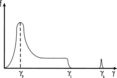
Figure 1: The distribution function versus the Lorentz factor. As is clear from the plot, the function consists of two parts: the first - wider region concerns the plasma component corresponding to the cascade processes of pair creation and the second one characterizes the primary Goldreich-Julian beam electrons.

2 Centrifugally Driven Langmuir Waves in the Pulsar magnetosphere

To develop a model for the centrifugally induced parametric Langmuir instability, we will assume that the magnetic field lines are almost rectilinear- a good approximation for distances less than the curvature radius of the field lines. Then in the rotating frame of straight field lines co-rotating with the pulsar, the metric is given by

$$ds^{2}=c^{2}\left(1-\frac{\Omega^{2}r^{2}}{c^{2}}\right)dt^{2}-dr^{2}.$$ (1)

In the $1+1$ formalism (Thorn et al., 1986) for a single particle, the particle equation of motion, in the rotating frame of reference, reads

$$\frac{d{\bf p}_{i}}{d\tau}=\gamma_{i}{\bf g}+\frac{e_{i}}{m}\left({\bf E}+\frac{1}{c}\bf v_{i}\times\bf B\right),$$ (2)

where ${i}=e,p$ is the species index, $e_{i}$ is the charge of the corresponding particle, $d\tau\equiv\xi dt$, $\xi\equiv\left(1-\Omega^{2}r^{2}/c^{2}\right)^{1/2}$ is the so-called time lapse function, ${\bf g}\equiv-{\bf\nabla}\xi/\xi$ is the gravitational potential, $\gamma_{i}\equiv\left(1-{\bf V}_{i}^{2}/c^{2}\right)^{-1/2}$ is the Lorentz factor, and ${\bf p}_{i}$ and ${\bf V}_{i}$ are, respectively, the dimensionless momentum (${\bf p}_{i}\rightarrow{\bf p}_{i}/m$) and velocity. The first term on the righthand side of the equation represents the centrifugal force, and plays a crucial role in our model.

To transport the equation of motion into the laboratory frame, we use the well known relation $\gamma=\xi\gamma^{\prime}$ connecting Lorentz factors in the rotating ($\gamma$) and laboratory ($\gamma^{\prime}$) frames. The identity $d/d\tau\equiv\partial/\partial(\xi\partial t)+\left({\bf v\cdot\nabla}\right)$ takes Eq. (2) into the laboratory frame

$$\frac{\partial{\bf p}_{i}}{\partial t}+({\bf v_{i}\cdot\nabla)p}_{i}=$$

$$=-c^{2}\gamma_{i}\xi{\bf\nabla}\xi+\frac{e_{i}}{m}\left({\bf E}+\frac{1}{c}\bf v_{i}\times\bf B\right),$$ (3)

where we have omitted the primes for notational simplicity. Note that the first term, originating in the relativistic effects of co-rotation, has a singular behavior on the light cylinder surface (a hypothetical zone, where the linear velocity of rotation exactly equals the speed of light). Throughout the area of interest, the overall effect of the term $c^{2}\gamma_{i}\xi{\bf\nabla}\xi$ will be significant.

Equation (2) is clearly fluid-like. In order to motivate this change in appearance, we need to make a digression. The plasma we plan to describe is really a kinetic fluid, the distribution function covers a wide range of $\gamma$ (energy) and as will later insist, a variable phase. A proper detailed description, then, is rather involved and will require numerical modeling. In this paper, however, we plan to extract our main results in a highly reduced description. We will assume that the plasma is multi-stream, each stream with a characteristic $\gamma$ and a characteristic phase. Then we will solve the linear ”interacting” dynamics of two such streams and demonstrate how a very interesting manifestation of the two stream instability takes place; the phase difference between the streams will emerge as the driver. Each stream, of course, is an electron-positron plasma. Equation (2), then, is to be viewed as equation of motion of the specie i(electron or positron) in a given stream, and along with the continuity equation

$$\frac{\partial n_{i}}{\partial t}+{\bf\nabla}\cdot\left(n_{i}{\bf v_{i}}\right)=0$$ (4)

and the Poisson equation

$${\bf\nabla\cdot E}=4\pi\sum_{i}e_{i}n_{i}.$$ (5)

completes the dynamics.

The centrifugal force (Machabeli & Rogava, 1994) is the cause of equilibrium or background velocity for the stream particles. The electromagnetic terms do not contribute (to the equilibrium) because of the frozen-in condition ${\bf E_{0}+v_{0i}\times B_{0}=0}$. In equilibrium, Eq. (2) reads (Machabeli & Rogava, 1994)

$$\frac{d^{2}r}{dt^{2}}=\frac{\Omega^{2}r}{1-\frac{\Omega^{2}r^{2}}{c^{2}}}\left[1-\frac{\Omega^{2}r^{2}}{c^{2}}-\frac{2}{c^{2}}\left(\frac{dr}{dt}\right)^{2}\right].$$ (6)

For highly relativistic particles ($\gamma\gg 1$), Eq. (6) yields the simple periodic solution,

$$r(t)\approx\frac{V_{0}}{\Omega}\sin\left(\Omega t+\phi\right),$$ (7)

$$\upsilon_{0}(t)\approx V_{0}\cos\left(\Omega t+\phi\right).$$ (8)

The phase $\phi$, necessary to insure a general solution of Eq. (6), was taken to be zero in previous work (Machabeli et al., 2005). This was a very serious shortcoming because the zero phase solution applies only to a very small subset of particles. The nonzero phase will insure the inclusion of all particles in the dynamics. Consequently, the instability could feed on much of the population of the magnetospheric plasma resulting in very large growth rates .

The orbits (7,8), along with the frozen-in condition, provide the equilibrium input for the linear stability analysis. Since the calculated equilibrium is time dependent, the standard time -Fourier anaylsis will not pertain- the solution of the stability problem will be more involved and nuanced.

One begins with the standard splitting of the physical variables $\Psi=(n,{\bf v,p,E,})$ into equilibrium and perturbed parts

$$\Psi\approx\Psi^{0}+\Psi^{1},$$ (9)

The next step is somewhat different; the linear perturbations are expanded as

$$\Psi^{1}(t,{\bf r})\propto\Psi^{1}(t)\exp\left[i({\bf kr})\right],$$ (10)

where both the amplitude and the exponent are functions of time. To keep the notation simple, we will drop the superscript $1$ labelling perturbed quantities.

In the linearized version of Eqs. (2-5):

$$\frac{\partial p_{i}}{\partial t}+ik\upsilon_{0}p_{i}=\upsilon_{0}\Omega^{2}rp_{i}+\frac{e_{i}}{m}E,$$ (11)

$$\frac{\partial n_{i}}{\partial t}+ik\upsilon_{{i}0}n_{i},+ikn_{{i}0}\upsilon_{i}=0,$$ (12)

$$ikE=4\pi\sum_{i}e_{\beta}n_{i},$$ (13)

$E$ is the electrostatic field, and i is the species index. Notice that we have retained only the radial component of the linearized momentum equation, $p_{i}=\widehat{{\bf e}_{r}}\cdot{\bf p}_{i}$ and $k=\widehat{{\bf e}_{r}}\cdot{\bf k}$.

The electron-positron dynamics can be combined in terms of two fluid variables:, the relative velocity ${\bf v\equiv v_{e}-v_{p}}$, the differential density$n\equiv n_{e}-n_{p}$, the average fluid velocity ${\bf v_{e}^{0}\approx v_{p}^{0}\equiv v^{0}}$, and the mean density, $n_{e}^{0}=n_{p}^{0}\equiv n^{0}$. Thus for the two stream model (labelled by $\beta$=1,2), the linear system (11-13) takes the form,

$$\frac{\partial p_{\beta}}{\partial t}+ik\upsilon_{\beta 0}p_{\beta}=\upsilon_{\beta 0}\Omega^{2}rp_{\beta}+\frac{2e}{m}E,$$ (14)

$$\frac{\partial n_{\beta}}{\partial t}+ik\upsilon_{{\beta}0}n_{\beta},+ikn_{{\beta}0}\upsilon_{\beta}=0$$ (15)

$$ikE=4\pi e\sum_{\beta}n_{\beta 0};$$ (16)

the two streams being coupled through the Poisson equation. We remind the reader that the two-stream model was invoked, very crudely, to capture the essence of the vast spectrum in energy and initial orbit phase available to the plasma particles. Each stream carries its own $\gamma$ and phase $\phi$.

Equations (14-16), due to the time dependence of the orbits ($r$, and $v_{0}$), represent a set of non-autonomous differential equations. The goal is to determine if an arbitrary perturbation will grow in time. We will follow two complementary methodologies to establish the existence of an instability and to determine the growth characteristics; an exact numerical solution and an approximate analytical estimate via a quasi-modal approach.

We convert (14-16) into two coupled equations

$$\frac{d^{2}N_{1}}{dt^{2}}+{\omega_{1}}^{2}N_{1}=-{\omega_{1}}^{2}N_{2}e^{i\chi}$$ (17)

$$\frac{d^{2}N_{2}}{dt^{2}}+{\omega_{2}}^{2}N_{2}=-{\omega_{2}}^{2}N_{1}e^{-i\chi}$$ (18)

in terms of the perturbed ”densities’

$$N_{\beta}=n_{\beta}e^{\frac{ick}{\Omega}\sin\left(\Omega t+\phi_{\beta}\right)},$$ (19)

where we have replaced $V_{0}$ by $c$. The frequencies $\omega_{1,2}\equiv\sqrt{8\pi e^{2}n_{1,2}/m\gamma_{1,2}^{3}}$ are, respectively the effective relativistic plasma frequencies (for longitudinal modes) corresponding to the two streams, and

$$\chi=\frac{ck}{\Omega}[\sin(\Omega t+\phi_{1})-\sin(\Omega t+\phi_{2})]=b\cos(\Omega t+\phi_{+})$$ (20)

with $2\phi_{\pm}=\phi_{1}\pm\phi_{2}$, and

$$b=2\frac{ck}{\Omega}\sin\phi_{-}$$ (21)

In deriving Eqs.(17-18), we have invoked $(ck/\Omega)>>1$ to drop the first term on the right hand side of Eq. (14). This parameter will turn out to be approximately the ratio of the Langmuir frequency to the star rotation frequency and will lie in the range $10^{6}-10^{10}$.

The evolution Eqs.(17-18) with definitions (20-21) have the following features:

1) The evolution of the two streams is coupled.

2) The time dependence of the coefficients is fully contained in $\chi$.

3) $\chi$ depends on both the sum and difference of the phases associated with the two streams.

4) The dependence on the phase sum $2\phi_{+}=\phi_{1}+\phi_{2}$ is trivial. In fact it can be absorbed in a redefinition of time variable; $\phi_{+}$ will be dropped from now on.

5) The phase difference $\phi_{-}$, however, is a fundamental parameter of the two-strem system and determines the magnitude of $\chi$. For $\phi_{-}=0$, $\chi\approx 0$, Eqs.(17-18) reduce to an autonomous system with constant coefficients and lead to the modal dispersion relation ${\omega}^{2}={\omega_{1}}^{2}+{\omega_{2}}^{2}$. The two streams collapse to one since $\phi_{-}$, the ”measure” of their difference, has gone to zero. Strictly speaking, this is only an approximation, since in Eq. (20) we have assumed $V_{0\beta}=c$, whereas $V_{0\beta}\approx c\left(1-\frac{1}{2\gamma_{0\beta}}\right)$. Without this approximation, we will get a nonzero growth rate even for $\phi_{-}=0$). However, this vestigial growth rate is many orders of magnitude smaller than what we will obtain for finite $\phi_{-}$.

We would reassert that introducing the initial phase is a fundamental departure from earlier work. It is the phase difference that differentiates the two streams and sets the stage for a strong two stream instability.

We will first perform a time Fourier analysis to search for a growing quasi mode (for non autonomous systems there are no fourier modes). We must manipulate Eqs.(17, 18) to yield

$$\frac{d^{2}N_{2}}{dt^{2}}=\frac{{\omega_{2}}^{2}}{{\omega_{1}}^{2}}e^{-i\chi}\frac{d^{2}N_{2}}{dt^{2}}.$$ (22)

We, then, use the Bessel identity

$$e^{\pm ib\sin y}=\sum_{\mu}J_{\mu}(b)e^{\pm i\mu y},$$ (23)

and take the Fourier transform of Eqs.(17-22) to derive the relation

$$(\omega^{2}-\omega_{1}^{2})N_{1}(\omega)=\omega_{2}^{2}\sum_{\mu\nu}Q_{\mu}^{+}Q_{\nu}^{-}\frac{(\omega+(-\mu+\nu)\Omega)^{2}}{(\omega-\mu\Omega)^{2}}N_{1}(\omega+(-\mu+\nu)\Omega)$$ (24)

where

$$Q_{\mu}^{\pm}=e^{\pm i\mu\frac{\pi}{2}}J_{\mu}(b)$$

Equation (24) is clearly not a dispersion relation, each Fourier component (labeled by $\omega$) is connected to all other components. In spite of the formidable double sum on the right hand side, we can still extract useful information that will establish the possibility of the growth of perturbations. An indicative ” dispersion relation ”relation may be obtained by keeping terms with $\nu=\mu$

$$\omega^{2}-\omega_{1}^{2}-\omega_{2}^{2}J_{0}^{2}(b)=\omega_{2}^{2}\sum_{\mu}J_{\mu}^{2}(b)\frac{\omega^{2}}{(\omega-\mu\Omega)^{2}}.$$ (25)

We make further analytical progress by simply keeping a single resonant term defined by the harmonic of the star rotation frequency that is in resonance with the real part of the mode frequency, $\omega_{r}=\mu_{res}\Omega$ where $\omega=\omega_{r}+\Delta$ ( $\Delta<<\omega_{r}$). After some straightforward algebra, one can derive

$$\Delta^{3}=\frac{\omega_{r}{\omega_{2}}^{2}{J_{\mu_{res}}(b)}^{2}}{2},$$ (26)

implying an imaginary part- growth rate:

$$\Gamma=\frac{\sqrt{3}}{2}\left(\frac{\omega_{r}{\omega_{2}}^{2}}{2}\right)^{\frac{1}{3}}{J_{\mu_{res}}(b)}^{\frac{2}{3}}.$$ (27)

The preceding analytical calculation, though simple and revealing, should be taken only as an indicator that the Langmuir waves (charge separation perturbations) can grow in time transferring energy from pulsar rotation to the electric field. As remarked earlier the instability is an appropriate version of the two-stream instability in which both streams move with speeds close to $c$, but whose constituent particles start with different initial orbits-the difference manifesting itself through the phase factor $\phi_{-}$.

The expression (27) for the growth rate tells us that, apart from its dependence on $\omega_{1}$ and $\omega_{2}$, the growth rate is controlled by the Bessel function $J_{\mu_{res}}(b)=J_{\mu_{res}}((2ck/\Omega)\sin\phi_{-})$ of very high order $\mu_{res}=\omega/\Omega\gg 10^{4}$. Bessel functions of such high order are vanishingly small unless the argument $(2ck/\Omega)\sin\phi_{-})\approx\mu_{res}$. For $\phi_{-}$ approaching zero, the growth rate becomes vanishingly small (Machabeli et al., 2005).

We could readily make analytical estimates for the growth rate of the rotationally driven Langmuir waves for a typical pulsar. However we must bear in mind that these estimates can be merely suggestive since the fundamental dynamics is non-autonomous in time and a given Fourier mode cannot capture the time behavior. It is particularly so because $\mu_{res}$ is so large that a whole band of harmonics will contribute to the sum (24) even if mode coupling were neglected. However, the evolution of each mode is governed by others and the time asymptotic response does depend on the coupling of Fourier modes- we must deal with the entire wave packet.

Fortunately the system of Eqs.(17-18), with periodic coefficients, is readily amenable to a simple numerical solution for the densities $N_{1}$ , $N_{2}$ (and the electric field, $E=N_{1}-N_{2}e^{i\chi}$). Differential equations with periodic coefficients (Mathieu equation being the simplest example) are known to display parametric instabilities in well defined regimes. Mathematica solutions demonstrate that model Eqs.(17-18) are, indeed, parametrically unstable and acquire a hefty growth rate when $b\approx\omega/\Omega$ (this behavior was predicted by the analytical dispersion relation). It turns out the time asymptotic behavior, for cases of interest, does settle into a pattern that growth rate of the instability can be read off from the time evolution graph. We shall soon see that rotation (centrifugally) driven Langmuir waves can grow at a very fast rate.

3 Discussion

We shall now explore the detailed characteristic of the centrifugally driven Langmuir waves for the crab pulsar. Our eventual aim is to put together a mechanism for delivering the rotational slow down energy to particle acceleration. It will happen in two major steps: (I) in the first stage, by means of the centrifugally induced parametric instability, the pulsar’s rotation energy is transferred to the electrostatic waves; (II) and in the second stage the amplified electrostatic modes undergoes Landau damping on high energy electrons causing efficient particle acceleration.

3.1 Centrifugally induced Langmuir waves

In order to make reasonable estimates for the instability growth rate, we recapture some details of our model. What we are studying is the instability that arises in a highly relativistic electron-positron plasma in the pulsar magnetosphere. We have modeled the plasma in terms of two distinct streams distinguished by their $\gamma$ factors and the initial orbit phase (we have assumed the speed of both streams to be c). Let the two streams have quite different $\gamma$s with $\gamma_{1}<\gamma_{2}$. The frequencies $\omega_{1,2}$ are calculated from the stream densities and $\gamma_{1,2}$. Assuming that energy is uniformly distributed throughout the magnetospheric plasma, we may approximate $n_{1}\gamma_{1}\approx n_{2}\gamma_{2}\approx n_{b}\gamma_{b}$, where $n_{b}=n_{{}_{GJ}}=\Omega B/(2\pi ec\xi^{2})$ is the Goldreich-Julian number density (Ruderman & Sutherland, 1975). The magnetic field (on the light cylinder zone) $B=B_{st}(R_{st}/r_{0})^{3}$ is related to $B_{st}\approx 6.7\times 10^{12}$, the magnetic field close to the neutron star’s surface. With these density relations, we conclude that one of the parameters for the numerical solution, $\alpha={\omega_{2}}^{2}/{\omega_{1}}^{2}={\gamma_{1}}^{4}/\gamma_{2}^{4}$ will be much smaller than unity. The most important determining parameter of the system, however, is $w=\omega_{1}/\Omega$, the ratio of the rotation frequency to the mode frequency ($\approx\omega_{1}$); the parameter $w$ will lie, typically, between $10^{6}-10^{10}$, the former near the light cylinder and the latter near the pulsar surface. Specifying $\alpha$, $w$, $b$, and the initial conditions is sufficient to seek a numerical solution. The parameter $b$ is set by the wave number k and the phase difference $\phi_{-}$. From the general character of the differential equations, we expect strong parametric amplification when $b\geq w$.

From our extensive numerical study, we pick up two representative Mathematica plots (Fig. 2 and Fig. 3). In these, the solutions for $ReN_{1}$, $ImN_{I}$, $ReN_{2}$, and $ImN_{2}$ are plotted as functions of time. Time has been normalized to the inverse of the frequency $\omega_{1}$, the relativistic plasma frequency corresponding to the stream with lower $\gamma$ and much higher density. The respective parameters for the two figures are: For Fig. 2, $w=b=10^{7}$, $\alpha=.01$, and for Fig. 3, $w=b=10^{8}$, $\alpha=.01$. Since the $x$ axis denotes time measured in their respective plasma time (inverse of $\omega_{1}$)- the ”absolute” time scales in the two figures are different by a factor $\sqrt{10}$. For each case, we choose initial conditions(t=0) for what we call the Sin solution: $N_{1}(0)=0,{N_{1}}^{\prime}(0)=1,N_{2}(0)=0,{N_{2}}^{\prime}(0)=\alpha(\cos{b}-i\sin{b})$; it is easy to verify that these constitute a consistent solution to the coupled differential equations in the limit $t\rightarrow 0$.

The principle results of the numerical investigations may be summarized as:

a) For initial times $t/w<<1$(not displayed in the figures), the streams are essentially uncoupled and each oscillates at its own plasma frequency; the frequencies are real. Since $w$ is large, this stage can be reasonably long. For the two cases displayed, the period lasts $\approx 3.10^{4}$ plasma periods for case 1, and $\approx 2.10^{5}$ plasma periods for case 2. In each case the period is $\approx 10^{-3}$ of the star rotation period. Compared to the star rotation time, the coupling and instability build-up time is very small for the displayed examples.

b)As long as $b\ll w$, even for large $t/w$, the coupling between the streams remains small. Consequently, the perturbations amplitudes remain limited.

c) As $b$ approaches $w$, the two streams begin to interact after some initial lapse of time and all 4 amplitudes begin to grow. Since the two streams are assumed to have different intrinsic plasma frequencies ($\alpha={\omega_{2}}^{2}/{\omega_{1}}^{2}={\gamma_{1}}^{4}/\gamma_{2}^{4}<<1$) the time dependence of ($ReN_{1},ImN_{1})$, and ($ReN_{2},ImN_{2})$ are quite different. It can be seen from the figures that although ($ReN_{1},ImN_{1})$ oscillate (at a new slow frequency, the plasma oscillations are very fast and ever present-not resolved in the pictures) and grow, the amplitudes ($ReN_{2},ImN_{2})$ simply grow. Interestingly enough, the slow time evolution is exponential as predicted by the Floquet theory of differential equations with periodic coefficients. Thus the amplitude of entire perturbation (not just a given Fourier mode) exponentiates, and one can define a ”global” growth rate.

d) From the numerical solutions one can readily extract the the growth (exponentiation) time. For the solution in Fig. 2, it is $\approx 2000$ plasma times $\approx 2.10^{-4}P$, while the growth rate for the solution in Fig. 3 is $\approx 6000$ plasma times $\approx 6.10^{-5}P$, where $P$ is the pulsar period. Thus once the instability sets in, its growth rates are very high compared to the frequency of star rotation.

e) For a given $b$ and $w$, the growth rates go down as ${\alpha}^{1/3}=(\gamma_{1}/\gamma_{2})^{4/3}$, precisely the scaling implied in the simple analytical estimate (27). Given that the growth rates are quite high, one may conclude that even the streams with quite disparate $\gamma$ would produce a hefty instability.

f) For a moderate and not too small $\alpha$, the primary determinant of the instability gestation time, and growth rate is the relative value of $b=2ck/\Omega\sin\phi_{-}$ and $w=\omega_{1}/\Omega$. Both $\omega_{1}$ and $\Omega$ are determined by the pulsar phenomenology and are independent of the wave characteristics. Thus to bring $b$ to the range of strong instability, one has to choose $k\sin\phi_{-}$ to be in the desirable range. In principle, then, for any finite $\sin\phi_{-}$, one can find a range of $k$ for strong growth. The centrifugal drive for Langmuir waves is, therefore, very robust and effective over a wide spectrum.

g)The two stream model calculation, though far from perfect, is perfectly capable of capturing the essence of the pumping of Langmuir waves in the magnetospheric electron-positron plasma by the star rotation. A more detailed and comprehensive semi-kinetic model, that treats $\gamma$ and $\phi_{-}$ as phase space variables, is certainly recommended. However the current calculation creates a strong basis for the rapid build-up of rotationally pumped Langmuir waves (and their associated longitudinal electric fields) so that we can confidentlly begin to explore the consequences of these electric fields for particle acceleration.

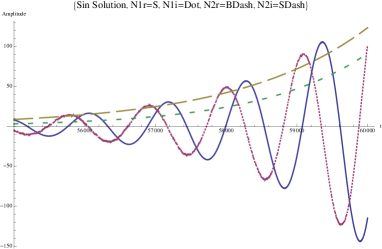
Figure 2: The temporal behaviour of amplitudes of $ReN_{1}$ (S), $ImN_{1}$ (Dot), $ReN_{2}$ (BDash), $ImN_{2}$ (SDash).

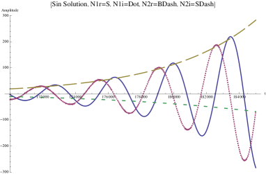
Figure 3: The temporal behaviour of amplitudes of $ReN_{1}$ (S), $ImN_{1}$ (Dot), $ReN_{2}$ (BDash), $ImN_{2}$ (SDash).

3.2 Particle acceleration

After having established that the rotational energy of the pulsar can be rapidly converted into charge separation electrostatic fields, we will now address the next issue of driving fast particles with these electric fields. Looking for a mechanism to produce super- energetic particles, we will concentrate on further energizing the most energetic particles in the pulsar atmosphere- the primary beam electrons that, to begin with, have rather high Lorentz factors as high as $\gamma_{b}\sim 10^{7}$ (Osmanov & Rieger, 2009).

The principal energy transfer (from waves to particles) channel explored in this work is the damping of Langmuir waves on electrons (Landau damping). Landau damping is, primarily, a kinetic process and will need to be appropriately integrated into what has been, till now, an essentially fluid approach. Even at the cost of repetition, it helps to emphasize that, in our model,

1) The Langmuir waves are produced by the bulk e-p plasma characterized by the relatively lower $\gamma$ region of the distribution (Fig.1),

2) while we want these waves to damp on the electron beam that appears as a small blip in the very high $\gamma$ end of the spectrum (Fig.1)

The ”producer” and the expected ”consumer” particles, though sharing the same physical space, are very different in their numbers, and in per particle intrinsic energy.

The study of electrostatic waves in ultrarelativistic plasmas started prior to the discovery of pulsars (Silin, 1960; Tsitovich, 1961), but gained considerable momentum after the discovery (Lominadze et al., 1979; Volokitin et al., 1987). From this set of papers, one learns that (one dimensional) electrostatic waves in relativistic e-p plasmas allow very simple dispersion in two limits: when the phase velocity is very high ($\upsilon_{ph}\equiv\omega_{r}/k\gg c$), and when the phase speed is very close to the speed of light, $\upsilon_{ph}\approx c$. It is clearly the second case that is of interest to the energy transfer mechanism. In this limit, the real part of the dispersion relation takes the form (Lominadze et al., 1979)

$$\omega=kc-\beta(k-k_{0}),$$ (28)

where $\beta=\langle\gamma\rangle/\langle 2\gamma^{3}\rangle$ is a very small parameter $\langle\rangle$ denotes momentum averaging), and $k_{0}$ is the limiting value of $k$ for which the phase speed is exactly $c$. From Eq. (28), we infer that the phase velocity will be less than the speed of light if $k>k_{0}$; this condition defines the regime in which such a wave could strongly interact with physical particles.

Going back to the unstable Langmuir waves, described in the previous section, we recall that the instability growth rates were found to be highest when the parameter (argument of the Bessel function) $(2ck/\Omega)\sin\phi_{-}$ is close to but moderately greater than $\mu_{res}$ (the order of the Bessel function). The ”resonance” condition,

$$(2ck/\Omega)\sin\phi_{-}\approx g\mu_{res}=g\omega/\Omega$$ (29)

where g is number $\geq 1$, implies that the phase velocity of the unstable waves, $\omega/k=\upsilon_{ph}\approx(2c/g)\sin\phi_{-}$, is in the correct regime as long as $2\sin\phi_{-}/g$ is close to but less than unity. For g=1, for example, only the waves generated by streams whose phase difference, $\phi_{-}\leq\pi/6$, will be able to accelerate particles; the highest growth pertain for waves for which $\phi_{-}$ is asymptotically close to $\pi/6$ and the phase velocity of such waves is asymptotically close to $c$.

Thus the e-p bulk plasma, preferentially, generates waves with phase velocity asymptotically approaching $c$. These waves will, preferentially, react with particles that move very close to the speed of light. In the pulsar magnetosphere, the primary beam particles (the narrow blip on the high $\gamma$ end of the distribution function shown in Fig. 1), belong to the most relativistic class. The Langmuir waves, therefore, would, preferentially damp on them. Indeed, Eq. (28) tells us that closer the phase velocity to $c$, the smaller the value of $\beta=\langle\gamma\rangle/\langle 2\gamma^{3}\rangle$, and, consequently the larger the value of required $\langle\gamma\rangle$.

To recapitulate the working of the Landau damping mechanism, let us place the phase velocity of the wave in that part of the primary beam region in which the distribution function decreases with $\gamma$ ($\partial f/\partial p<0$ or $\partial f/\partial\gamma<0$). In this zone the number of electrons that satisfy $\upsilon_{b}<\upsilon_{ph}$ is more than the number of electrons with $\upsilon_{b}>\upsilon_{ph}$, $\upsilon_{b}$ denoting the electron speed. Less energetic particles will gain energy from the waves, whereas more energetic electrons will loose energy, but since the number of particles with $\upsilon_{b}<\upsilon_{ph}$ is more than that of particles with $\upsilon_{b}>\upsilon_{ph}$, the waves will damp with a net energy transfer to the beam electrons.

As an aside, the parametric instability, discussed here, may be different from the one conjured in a typical laboratory setting. In the pulsar magnetospheric situation, the plasma frequency exceeds the rotation frequency by many orders of magnitude. The resonance is possible only for higher order harmonics and with phase velocity slightly less than the speed of light.

From the relativistic plasma literature (Volokitin et al., 1987), we can read off the estimated characteristic damping rate (Volokitin et al., 1987)

$$\Gamma_{LD}=\frac{n\gamma\omega_{p}}{n_{1}\gamma_{1}^{5/2}},$$ (30)

where $n$, $\gamma$ and $\omega_{p}=\sqrt{4\pi e^{2}n/m}$ are respectively the number density, the Lorentz factor and the plasma frequency of the specie on which the damping occurs.

If the instability growth rates, and the Landau damping rates were very disparate, there will be little effective energy transfer from waves to the particles. On the other hand, if the damping rates were far in excess of the growth rates, the waves will not grow much, again resulting in very little transfer from the star rotation to the waves. The most optimum scenario for an overall efficient energy pumping/transfer system is realized when the instability growth and Landau damping rates are large and comparable, $\Gamma\sim\Gamma_{LD}$.

Since it is the electron-positron plasma that supports and feeds the two-stream instability, the corresponding characteristic energy in the unstable waves is of the order of the energy accumulated (transferred from star rotation) in the plasma components. Remembering that the number density associated with the e-p-plasma far exceeds that of the beam component (see Fig.1), the energy gained per beam electron could be extremely large if a substantial fraction of total “available” energy in plasma components were transferred via the electrostatic fields.

The condition $\Gamma\sim\Gamma_{LD}$ is satisfied, for instance, by the choice $\gamma_{2}=4700$, $\gamma_{1}\approx 800$ for the two streams. The resulting instability growth rate is of the order of $10^{4}$s^-1; the corresponding growth period of $10^{-4}s$ is several orders of magnitude less than the pulsar rotation period. The rate of energy transfer to the waves is extremely fast- the processes under consideration are extremely efficient.

Let us probe further into the details of energy transfer from the star rotation into the plasma particles. In the local frame of reference the particles are forced to slide along the magnetic field lines by means of the centrifugal force. Viewed in the laboratory frame, the reaction force $F_{reac}\approx 2mc\Omega\xi(r)^{-3}$ (Rogava et al., 2003), driving the particles, becomes infinite on the light cylinder surface. This is a natural result- to preserve rigid rotation, the particle velocity, in this region, must exactly equal the speed of light. Note also that the radial velocity tends to zero, because on the light cylinder the particles can only rotate with the linear velocity $c$. It is clear that the maximum energy gained from the rotator can be estimated as the work done by the reaction force. For all particles involved in the process, the energy gain may be estimated as ($n_{1}\gg n_{2}$)

$$W\approx n_{1}\delta VF_{reac}\delta r,$$ (31)

where $\delta V$ is the volume in which the pumping takes place and $\delta r\sim c/\Gamma$ is the corresponding lengthscale.

Since the aforementioned work done is transferred to the beam electrons in the same volume, the energy of a given beam particle $\epsilon$ can be approximately calculated by equating $W$ with the total energy gained by the accelerated beam particles, $n_{b}\delta V\epsilon$,

$$\epsilon\approx\frac{n_{1}F_{reac}\delta r}{n_{b}}.$$ (32)

One can readily show that, in the vicinity of the light cylinder surface ($\xi\sim 10^{-2}$), and for typical magnetospheric parameters, $n_{1}\approx 2.5\times 10^{11}$cm^-3, $n_{b}=n_{GJ}\approx 2\times 10^{7}$cm^-3, $\epsilon$, the energy acquired by a beam electron could get to be as very high- $100s$ of TeVs or higher.

Because the highly relativistic particles will, inevitably, loose energy due to radiation, one must investigate how radiation will affect overall energy transfer. Could radiation, for example, put a stringent limit on the maximum energy acquired?

For highly relativistic electrons and photons with $\epsilon\epsilon_{ph}/(m^{2}c^{4})>1$ ($\epsilon_{ph}$ is photon energy), the inverse Compton mechanism operates in the Klein-Nishina (KN) regime(Rybicki & Lightman, 1979). Energy emitted per particle per second is, then, given by the approximate expression $P_{KN}\propto\pi r_{e}^{2}m^{2}c^{5}n_{ph}(\epsilon_{ph})\mid ln\left(4e\epsilon/m^{2}c^{4}-11/4\right)\mid$ (Blumenthal & Gould, 1970) where $r_{e}$ is the classical electron radius. The corresponding time scale of the process is $t_{KN}\sim\epsilon/P_{KN}$. Using the approximate photon number density, $n_{ph}(\epsilon_{ph})\approx L/4\pi R_{lc}^{2}c\epsilon_{ph}$ ($R_{lc}\equiv c/\Omega$ is the the light cylinder radius), and taking into account that for the Crab pulsar, $L\sim 10^{36}$erg/s, $\epsilon_{ph}\sim 100$GeV, it is straightforward to show that if $\epsilon=100$TeV (for instance), the aforementioned timescale exceeds the typical instability time scale ($t_{in}\sim 1/\Gamma$) by many orders of magnitude. Thus Compton cooling is very slow compared to the wave energy transfer time. The KN time scale goes up with the particle energy implying that at higher energies, the inverse Compton mechanism in the KN channel is tot slow to impose any constraints on the maximum attainable electron energy.

The next possible loss mechanism for relativistic particles, moving in magnetic field, is the synchrotron emission with the corresponding power $P_{syn}\approx 2e^{2}\omega_{B}^{2}\gamma^{2}/3c$ (Rybicki & Lightman, 1979), where $\omega_{B}\equiv eB/(mc)$ is the cyclotron frequency. One can readily show that the electrons leaving the gap with a $\gamma\sim 10^{6}$ will undergo so efficient synchrotron cooling that the corresponding time scale, $t_{syn}\sim\gamma mc^{2}/P_{syn}$ will be of the order of $10^{-21}$s. Thus, shortly after the particles leave the gap, they radiate their transverse momentum, and very soon transit to the ground Landau state. After that, zipping only along the field lines, the electrons will reach the light cylinder zone in due course of time. It is precisely the region, where the Langmuir waves, always propagating along the field lines, are excited. Therefore the wave interaction with particles will not cause pitch angle scattering, efficiently suppressing the synchrotron mechanism. Quasi linear diffusion, another possible source for imparting a pitch angle, (Lominadze et al., 1979), also does not operate because the required condition for diffusion $\omega_{B}>\omega_{1,2}$, is violated for extremely energetic plasmas (for plasmas with energy density exceeding that of magnetic field). The synchrotron mechanism, therefore, is not expected to impose any constraints on the maximum attainable energies.

How about the curvature radiation emitted by particles moving along the curved magnetic field lines? High energy electrons with energies in ($100s$ of TeVs), i.e, with particle energy density exceeding magnetic energy density by many orders of magnitude, move, practically, in a straight line. This in turn excludes the curvature radiation from interfering with our energy transfer mechanism. As in previous cases, curvature radiation ”does” not impose significant limits on $\epsilon$.

The absolute upper bound on the energy that an electron may acquire, may be estimated as follows: The total power budget, the slowdown luminosity, is $5.5\times 10^{38}$erg/s, about $40\%$ of which is radiated away by the Crab nebula. If the remaining $60\%$), $\Delta L\sim 3.5\times 10^{38}$erg/s, were fully used up (via the mechanism proposed in this paper) to accelerate electrons to ultra high energies, a beam electron could emerge with an energy

$$\epsilon\approx\frac{\Delta L}{4\pi\eta R_{lc}^{2}n_{GJ}c}\approx 1\frac{PeV}{\eta},$$ (33)

where $\eta<1$ is the fraction of particles involved in the process. Since the particles involved in the acceleration-radiation mechanisms, are from the region of open magnetic field lines, it is natural to assume that $\eta\ll 1$; this bunch of particles could be boosted up to multi PeV range. This estimate should be taken for what it is- an absolute upper bound. The most important message is that even if a very small percent of the total available energy could be transferred to fast electrons, the pulsar could be a source of ultra relativistic electrons with energies in the range of $100s$ of Tevs.

It is clear from the expression of $F_{reac}$ that the force increases asymptotically as we approach the light cylinder zone $\xi\rightarrow 0$. However, the projected singularity at the light cylinder surface may be circumvented by a recently conjectured mechanism: By means of a curvature drift instability, the magnetic field lines twist’ and, lagging behind the rotation, lead to the force-free dynamics of particles. The rigid rotation and the subsequent violation of the causality principle (Osmanov et al., 2009) is, thus, prevented. As a result, the process will, then, stop due to the aforementioned instability.

4 Summary

1. We have constructed a simple but nontrivial theoretical framework to explore the possibility of particle acceleration driven by the rotational slow down of a pulsar. The first step in the proposed mechanism is the conversion of the rotation imparted centrifugal particle energy, via a ”two stream instability”, to electrostatic Langmuir waves in the electron - positron plasma residing in the pulsar magnetosphere. Landau damping of these centrifugally excited electrostatic waves on the high energy primary beam electrons transiting through the same region, constitutes the second step.

2. By carrying out a linear instability analysis, relevant to a non-autonomous system, it was shown that, for physically reasonable parameters (pertinent for example to the Crab pulsar), the characteristic timescale for the growth of Langmuir waves is much less than the typical rotation timescales of particles. This means that the invoked instability is extremely efficient and can rapidly convert the star slow down energy into the electric field energy

3. Landau damping of the unstable Langmuir waves on primary beam electrons that converts the electric field energy into particle energy is also shown to be equally rapid. The combination creates a very efficient ”machine” that generates ultra high energy (multi TeV to PeVs) cosmic ray electrons; the star slow down luminosity being the ultimate accelerator.

The mechanism, developed in this paper, is rather general. The magnetospheres of active galactic nuclei (AGNs), for example, be just as suited to support centrifugally driven electrostatic waves. And these waves, could, equally efficiently, accelerate any charged leptons or hadrons.

Acknowledgements: The work of SMM was supported by USDOE Contract No.DE-FG03-96ER-54366.

References

- Abdo et al. (2009) Abdo, A.A. et al. 2009, Phys. Rev. L, 102, 181101
- Abramowitz & Stegun (1965) Abramowitz, M. & Stegun, I.A., 1965, Handbook of Mathematical Functions, Natl. Bur. Stand. Appl. Math. Ser. No. 55 (U.S. GPO, Washington, D.C., 1965)
- Ackermann et al. (2010) Ackermann, M. et al. 2010, Phys. Rev. D, 82, 092004
- Aharonian et at. (2008) Aharonian, F., et al. 2008, Phys. Rev. L, 101, 261104
- Arons & Sharleman (1979) Arons, J. & Sharleman, E.T., 1979, ApJ, 231, 854
- Blandford (1980) Blandford, R.D., 1980, ApJ, 238, 410
- Blandford & Ostriker (1980) Blandford, R.D. & Ostriker, J.P., 1980, ApJ, 237, 793
- Blumenthal & Gould (1970) Blumenthal, G. R. & Gould, R. J. 1970, Rev. Mod. Phys., 42, 237
- Chang et at. (2008) Chang, J. et al., 2008, Nature, 456, 362
- Deutsh (1955) Deutsh, A., 1955, Ann. Astrophys. 18, 1
- Goldreich & Julian (1969) Goldreich, P. & Julian, W.H., 1969, ApJ, 157, 869
- Kisaka & Kawanaka (2012) Kisaka, S. & Kawanaka, N., 2012, MNRAS, 421, 3543
- Lominadze et al. (1979) Lominadze J.G., Machabeli G.Z. & Mikhailovsky A.B., 1979, J. Phys. Colloq., 40, No. C-7, 713
- Lominadze et al. (1979) Lominadze, D.G., Mikhailovskii, A.B. & Sagdeev, R.Z., 1979, JETP, 50, 927
- Machabeli (1978) Machabeli, G.Z., 1978, SvJPP. 4, 914
- Machabeli et al. (2005) Machabeli, G., Osmanov Z. & Mahajan, S., 2005, Phys. Plasmas 12, 062901
- Machabeli & Rogava (1994) Machabeli, G.Z. & Rogava, A.D., 1994, Phys. Rev. A 50, 98
- Machabeli & Tsikarishvili (1978) Machabeli, G.Z. & Tsikarishvili, E.G., 1978, SvJPP. 4, 920
- Muslimon & Tsygan (1992) Muslimon, A.G. & Tsygan, A.I., 1992, MNRAS, 255, 61
- Osmanov & Rieger (2009) Osmanov, Z. & Rieger, F., 2009, A&A, 502, 15
- Osmanov et al. (2007) Osmanov, Z., Rogava, A.S. & Bodo G., 2007, A&A, 470, 395
- Osmanov et al. (2009) Osmanov, Z., Shapakidze, D. & Machabeli, Z. 2009, A&A, 503, 19
- Rieger & Mannheim (2000) Rieger, F. & Mannheim, K., 2000, A&A, 353, 473
- Rogava et al. (2003) Rogava, A., Dalakishvili, G. & Osmanov, Z., 2003, GReGr, 35, 1133
- Rybicki & Lightman (1979) Rybicki, G.B. & Lightman, A. P., 1979, Radiative Processes in Astrophysics. Wiley, New York
- Ruderman & Sutherland (1975) Ruderman, M.A. & Sutherland, P.G., 1975, ApJ, 196, 51
- Silin (1960) Silin, V.P., 1960, ZhETF, 38, 1577
- Sturrok (1971) Sturrok, P., 1971, ApJ, 164, 529
- Tademaru (1973) Tademaru, E., 1973, ApJ, 183, 625
- Thorn et al. (1986) Thorne, K., Price, R. & MacDonald, D.A., 1986, Black Holes: The Membrane Paradigm, (Yale University Press, New Haven, 1986)
- Tsitovich (1961) Tsitovich, V.N., 1961, ZhETF, 40, 1775
- Usov & Shabad (1985) Usov, V.V. & Shabad, A., 1985, ApSS, 117, 309
- Volokitin et al. (1987) Volokitin, A.S., Krasnoselskikh, V.V. & Machabeli, G.Z., 1987, Soviet Journal of Plasma Physics, 11, 310