Wetting in electrolyte solutions

Abstract

Wetting of a charged substrate by an electrolyte solution is investigated by means of classical density functional theory applied to a lattice model. Within the present model the pure, i.e., salt-free solvent, for which all interactions are of the nearest-neighbor type only, exhibits a second-order wetting transition for all strengths of the substrate-particle and the particle-particle interactions for which the wetting transition temperature is nonzero. The influences of the substrate charge density and of the ionic strength on the wetting transition temperature and on the order of the wetting transition are studied. If the substrate is neutral, the addition of salt to the solvent changes neither the order nor the transition temperature of the wetting transition of the system. If the surface charge is nonzero, upon adding salt this continuous wetting transition changes to first-order within the wide range of substrate surface charge densities and ionic strengths studied here. As the substrate surface charge density is increased, at fixed ionic strength, the wetting transition temperature decreases and the prewetting line associated with the first-order wetting transition becomes longer. This decrease of the wetting transition temperature upon increasing the surface charge density becomes more pronounced by decreasing the ionic strength.

I Introduction

Wetting transitions are surface phase transitions which occur whenever a phase C intrudes at the interface between two phases A and B, with either A, B, and C in thermodynamic coexistence or with A as a spectator phase and B and C in thermodynamic coexistence. As an example, A is an inert substrate and B and C are the gas and the liquid phase, respectively, of a simple fluid. The thickness of the intruding liquid film can be either finite (incomplete wetting) or macroscopically large (complete wetting) upon approaching gas-liquid coexistence along an isotherm. The transition at two-phase coexistence from incomplete to complete wetting occurs at the wetting transition temperature $T=T_{\text{w}}$. It can be either continuous (second-order), in which case the film thickness diverges smoothly as $T\to T_{\text{w}}$ along two-phase coexistence, or discontinuous (first-order), implying a macroscopically large jump of the film thickness from a finite value below $T_{\text{w}}$ to a macroscopically large one above $T_{\text{w}}$. In the surface phase diagram a first-order wetting transition has a prewetting line associated with it which is connected tangentially to the gas-liquid coexistence line at $T_{\text{w}}$, extends into the gas phase region, and ends at a critical point. The richness of wetting phenomena has been covered by various reviews deGennes ; Dietrich1988 ; Schick ; Bonn2001 ; Bonn2009 .

So far, to a large extent, wetting studies have been devoted to fluids composed of electrically neutral molecules. However, for numerous real systems the presence of ions is either of crucial importance for wetting phenomena, such as electrowetting Mugele , or unavoidable because many substrates release ions once they are brought into contact with polar solvents Everett . For example, electrowetting refers to the change of the substrate-fluid interfacial tension as a response to an applied electrostatic potential difference between the substrate and the fluid bulk. This effect offers numerous applications in devices based on the manipulation of tiny amounts of liquids, such as microfluidic devices pollack2000 ; Valev2003 . Theoretical studies of those systems started back in 1938 when Langmuir developed a model to determine the equilibrium thickness of water layers on planar surfaces in contact with undersaturated water vapor, based on the calculation of the repulsive force between two plates immersed in electrolyte solutions Langmuir1938 . The typical values for the equilibrium layer thickness as predicted by Langmuir’s formula were confirmed experimentally Hall1970 and the experimental data were used to analyze the effect of various contributions to the disjoining pressure onto the stability of the wetting films Derjaguin1974 . Some years later Kayser generalized Langmuir’s model for the equilibrium thickness of wetting layers to liquid mixtures of polar and non-polar components in contact with ionizables substrates Kayser1986 ; in contact with the wetting liquid these substrates donate ions to the liquid which act as counterions to the emerging opposite charge left on the substrate with overall charge neutrality. This analysis was followed up by including the effect of added salt the ions of which do not stem from the substrate Kayser1988 . These papers did not address the issue of wetting transitions at coexistence but rather focused on the thickness of the wetting layer and the behavior of the disjoining pressure. For wetting films of solvents without added salt, i.e., with counterions only, Langmuir Langmuir1938 and Kayser Kayser1986 found that the film thickness $l$ increases as $l\sim(\Delta\mu)^{-1/2}$, with $\Delta\mu=\mu_{co}-\mu$, as the chemical potential $\mu$ approaches its value $\mu_{co}$ at coexistence from the vapor side ($\mu<\mu_{co}$). In contrast, wetting films without ions and at neutral substrates but with van der Waals interactions (which are not taken into account in our model) lead to $l\sim(\Delta\mu)^{-1/4}$ or $l\sim(\Delta\mu)^{-1/3}$, depending on whether retardation effects are taken into account or not, respectively Dietrich1988 . In the case that the effect of added salt dominates van der Waals interactions Kayser Kayser1988 found $l\sim\ln(\Delta\mu)$ as it holds for short-ranged interactions.

Only recently theoretical investigations concerning wetting transitions of electrolyte solutions at charged solid substrates have emerged Denesyuk2004 ; Oleksy2009 ; Oleksy2010 . In Ref. Denesyuk2004 the effect of adding ions onto the wetting behavior of the pure solvent was studied by using Cahn’s phenomenological theory deGennes ; Dietrich1988 ; Schick ; Bonn2001 for the solvent combined with the Poisson-Boltzmann theory for the ions. This model does not take into account the solvent particles explicitly, neglecting the coupling between solvent particles and ions. On the other hand, the model in Ref. Oleksy2009 takes all three types of particles (solvent, cations, and anions) explicitly into account in terms of hard spheres of different diameters with a Yukawa attraction between all pairs and the Coulomb interaction between ions. The model was studied by using Rosenfeld’s density functional theory Rosenfeld1988 ; Rosenfeld1989 combined with a mean-field approximation for the Yukawa and the electrostatic interactions. Within this model, the polar nature of the solvent molecules was ignored; it was included in a subsequent article by the same authors in which the solvent particles were represented by dipolar hard spheres Oleksy2010 . However, for technical reasons, the numerical analyses of these continuum models in which all three types of particles are treated explicitly on a microscopic level were limited to small system sizes. Therefore Refs. Oleksy2009 ; Oleksy2010 focused on the case of strong screening of the Coulomb interactions which is provided by large ionic strengths, i.e., large ion concentrations. However, the approaches used in Refs. Denesyuk2004 ; Oleksy2009 ; Oleksy2010 are not reliable for large ionic strengths due to the use of Poisson-Boltzmann theory for the electrostatic interactions which has been proved to be valid only for low ionic concentrations Torrie1979 .

In order to overcome these problems we introduce a lattice model for an electrolyte exposed to a charged substrate which takes into account all three components via density functional theory and offers the possibility to study significantly broader interfacial regions. In Sec. II we introduce this model and the approximate density functional. In Sec. III we present our results for the bulk properties and the wetting phenomena for both the salt-free solvent and the electrolyte solution. We conclude and summarize our main results in Sec. IV.

II Model and density functional theory

II.1 Model

We study a lattice model for an electrolyte solution in contact with a charged wall. The solution consists of three components: solvent $(0)$, anions $(-)$, and cations $(+)$. The coordinate perpendicular to the wall is $z$. The region above the wall, accessible to the electrolyte components, is divided into a set of cells the centers of which form a simple cubic lattice $\{\bf r\}$ with lattice constant $a$. The volume $a^{3}$ of a cell corresponds roughly to the volumes of the particles, which are assumed to be of similar size. The centers of the molecules in the top layer of the substrate form the plane $z=0$. At closest approach the centers of the solvent molecules and ions are at $z=a$. The plane $z=a/2$ is taken to be the surface of the planar wall. Each cell is either empty or occupied by a single particle. This mimics the steric hard core repulsion between all particles. Particles at different sites interact among each other via an attractive nearest-neighbor interaction of strength $u$ which is taken to be the same for all pairs of particles. In addition, ion pairs interact via the Coulomb potential. The solvent particles are taken to carry a dipole moment.

The wall attracts particles only in the first adjacent layer via an interaction potential of strength $u_{\text{w}}$ which is the same for all species. In addition it can carry a homogeneous surface charge density $\tilde{\sigma}=\sigma ea^{-2}$ which is taken to be localized in the plane $z=a/2$ and which interacts electrostatically with the ions; $e>0$ is the elementary charge. Since we focus on the influence of the ions onto wetting phenomena we refrain from considering the more realistic, long-ranged van der Waals forces which are known to be relevant for wetting transitions Dietrich1988 . Within the mean-field theory we shall use, the choice of nearest-neighbor interactions provides a significant computational bonus which we want to exploit in favor of our core concern stated above.

The corresponding lattice-gas Hamiltonian for this system reads

$$\begin{split}H&=\frac{1}{2}\sum_{\begin{subarray}{c}{\bf r},{\bf r^{\prime}}\\ {\bf r}\neq{\bf r^{\prime}}\end{subarray}}\sum_{i,j}n_{i}({\bf r})n_{j}({\bf r^{\prime}})w\left(|{\bf r}-{\bf r^{\prime}}|\right)\\ &+\frac{1}{2}\sum_{\begin{subarray}{c}{\bf r},{\bf r^{\prime}}\\ {\bf r}\neq{\bf r^{\prime}}\end{subarray}}\sum_{i,j}\frac{e^{2}q_{i}q_{j}n_{i}({\bf r})n_{j}(\bf{r\,^{\prime}})}{4\pi\varepsilon_{0}|{\bf r}-{\bf r^{\prime}}|}\\ &+\sum_{\begin{subarray}{c}{\bf r},{\bf r^{\prime}}\\ {\bf r}\neq{\bf r^{\prime}}\end{subarray}}\sum_{i,j}\frac{eq_{i}n_{i}({\bf r}){\bf m_{j}({\bf r^{\prime}})\cdot({\bf r}-{\bf r^{\prime}})}}{4\pi\varepsilon_{0}|{\bf r}-{\bf r^{\prime}}|^{3}}\\ &+\frac{1}{2}\sum_{\begin{subarray}{c}{\bf r},{\bf r^{\prime}}\\ {\bf r}\neq{\bf r^{\prime}}\end{subarray}}\sum_{i,j}\left[\frac{{\bf m}_{i}({\bf r})\cdot{\bf m}_{j}({\bf r^{\prime}})}{4\pi\varepsilon_{0}|{\bf r}-{\bf r^{\prime}}|^{3}}\right.\\ &\left.-\frac{3\left({\bf m}_{i}({\bf r})\cdot({\bf r}-{\bf r^{\prime}})\right)\left({\bf m}_{j}({\bf r^{\prime}})\cdot({\bf r}-{\bf r^{\prime}})\right)}{4\pi\varepsilon_{0}|{\bf r}-{\bf r^{\prime}}|^{5}}\right]\\ &-\sum_{{\bf r}}\sum_{i}u_{\text{w}}\delta_{z,a}n_{i}({\bf r})-\frac{\tilde{\sigma}}{2\varepsilon_{0}}\sum_{{\bf r}}\sum_{i}q_{i}n_{i}({\bf r})z\\ &-\frac{\tilde{\sigma}}{2\varepsilon_{0}}\sum_{{\bf r}}\sum_{i}{\bf m}_{i}({\bf r})\cdot\hat{\bf e}_{z}\end{split}$$ (1)

where $n_{i}({\bf r})$ are occupation number variables, which are either 0 or 1 according to whether the cell at the discrete position ${\bf r}=({\bf r_{||}},z\geq a)=(x,y,z\geq a)=(ma,na,pa)$ with $m,n\in\mathbb{Z}$, $|m|\leq\bar{M}/2$ and $|n|\leq\bar{N}/2$, and $p=1,2,3,\cdots,\bar{L}$ is empty or occupied by a particle (there is no double occupancy); $i,j=0,+,-$, $eq_{i}$ is the particle charge with $q_{0}=0$ and $q_{\pm}=\pm 1$; ${\bf m_{i}}({\bf r})$ is the particle dipole moment at ${\bf r}$ (we consider the typical situation of a polar solvent and of ions without permanent electric dipoles, i.e., ${\bf m_{\pm}}=0$); $w\left(|{\bf r}-{\bf r^{\prime}}|\right)=-u$ for nearest neighbors ($u>0$ corresponds to attraction) and $w\left(|{\bf r}-{\bf r^{\prime}}|\right)=0$ beyond; $-u_{\text{w}}$ is the strength of the attractive ($u_{\text{w}}>0$) substrate potential acting on the first layer $z=a$. For the charge density $\tilde{\rho}({\bf r})=\tilde{\sigma}\delta(z-a/2)$ on a substrate with radial extension $R_{0}$ the electrostatic potential is given by $\tilde{\phi}({\bf r})=\int{\!d^{3}r^{\prime}\!\tfrac{\tilde{\rho}({\bf r^{\prime}})}{4\pi\varepsilon_{0}|{\bf r}-{\bf r^{\prime}}|}}=\tfrac{\tilde{\sigma}}{2\varepsilon_{0}}(\sqrt{R_{0}^{2}+(z-a/2)^{2}}-|z-a/2|)\to-\tfrac{\tilde{\sigma}}{2\varepsilon_{0}}z+const.$ for $R_{0}\gg|z-a/2|$ and $z>a/2$. In this regime of being close to the charged wall the electric field is uniform Jackson . Therefore the actual position of the charged wall enters the electrostatic potential, and thus the Hamiltonian in Eq. (1), only via an irrelevant additive constant. The potential energy of a dipole moment ${\bf m}_{i}({\bf r})$ in the electric field $\tilde{\bf E}({\bf r})=\tilde{\nabla}\tilde{\phi}({\bf r})\to\tfrac{\tilde{\sigma}}{2\varepsilon_{0}}\hat{\bf e}_{z}=const.$ of the surface charge is given by $-{\bf m}_{i}({\bf r})\cdot\tilde{\bf E}$. In Eq. (1) we consider only charge neutral configurations $\{n_{i}({\bf r})\}$, i.e., $\sum\limits_{\bf r}\left(n_{+}({\bf r})-n_{-}({\bf r})\right)=-\bar{M}\bar{N}\sigma$ with ${\bf r}\in V=\bar{M}\bar{N}\bar{L}a^{3}$.

For weak external electric fields the polarization is expected to exhibit a linear response behavior Jackson . In this case, it has been shown that the relative permittivity $\varepsilon$ of microscopic models like the one in Eq. (1) can be expressed in terms of molecular properties such as the dipole moment and the polarizability Wertheim ; Carnie . In order to simplify our model, the polar nature of the solvent is taken into account effectively via the relative permittivity $\varepsilon$ of the electrolyte solution which is assumed to depend on the solvent configuration $n_{0}({\bf r})$ but not on the configuration of the ions $n_{\pm}({\bf r})$ because the orientational polarization, i.e., the polarization due to the permanent dipoles of the solvent molecules, is the dominant contribution to the total polarization. In this case Eq. (1) reduces to (see, c.f., Eqs. (7) and (9))

$$\begin{split}H&=\frac{1}{2}\sum_{\begin{subarray}{c}{\bf r},{\bf r^{\prime}}\\ {\bf r}\neq{\bf r^{\prime}}\end{subarray}}\sum_{i,j}n_{i}({\bf r})n_{j}({\bf r^{\prime}})w\left(|{\bf r}-{\bf r^{\prime}}|\right)\\ &-\sum_{\bf r}\sum_{i}u_{\text{w}}\delta_{z,a}n_{i}({\bf r})\\ &+\frac{1}{2}\int_{V}\!d^{3}r^{*}\tilde{\phi}({\bf r^{*}})\tilde{Q}({\bf r^{*}})\end{split}$$ (2)

where $\tilde{Q}({\bf r^{*}})=\frac{e}{a^{3}}\sum\limits_{i}q_{i}n^{*}_{i}({\bf r^{*}})+\tilde{\sigma}\delta(z^{*}-a/2)$ is the local charge density where $n^{*}_{i}({\bf r^{*}})=n_{i}({\bf r})$ for all ${\bf r^{*}}\in(a\mathbb{R})^{3}$ and ${\bf r}\in(a\mathbb{Z})^{3}$ with $\max\left(|x^{*}-x|,|y^{*}-y|,|z^{*}-z|\right)\leq a/2$; $\tilde{\phi}({\bf r^{*}})$ is the electrostatic potential which can be obtained by solving the Poisson equation

$$-\varepsilon_{0}\tilde{\nabla}\cdot[\varepsilon(n^{*}_{0}({\bf r^{*}}))\tilde{\nabla}\tilde{\phi}({\bf r^{*}})]=\tilde{Q}({\bf r^{*}},[n^{*}_{\pm}]),\ \ \ \ \ {\bf r^{*}}\in(a\mathbb{R})^{3}\cap V,$$ (3)

where $V$ is the volume of the fluid. For general permittivity profiles $\varepsilon(n^{*}_{0}({\bf r^{*}}))$ no closed solution $\tilde{\phi}({\bf r^{*}})$ of Eq. (3) as a functional of $\varepsilon(n^{*}_{0}({\bf r^{*}}))$ and $\tilde{Q}({\bf r^{*}})$ is known, i.e., for each configuration $\{n_{i}({\bf r})\}$ the evaluation of Eq. (2) requires to solve the differential equation (3) anew. It has been proven, that models including charges as in Eq. (2) possess a proper thermodynamic limit for sequences of finite-sized systems, which is independent of the shape of the container, provided that globally charge neutral configurations $\{n_{i}(\bf r)\}$ are considered Lebowitz ; Lieb . Since the thermodynamic limit is performed for sequences of finite-sized systems the electrostatic potential $\tilde{\phi}({\bf r^{*}})$ in Eq. (3) vanishes at infinity ($|{\bf r^{*}}|\to\infty$) Jackson .

II.2 Density functional

With a given expression for $\varepsilon(n_{0}({\bf r}))$ (see, c.f., Eq. (15)), Eq. (2) can be used directly for numerical analyses such as Monte Carlo simulations, provided an efficient method to determine the electrostatic potential $\tilde{\phi}({\bf r^{*}})$ for arbitrary permittivity profiles $\varepsilon(n_{0}({\bf r}))$ becomes available (see for example Ref. Xu for recent efforts in this direction). We leave this challenging task for future studies. Here, we consider a suitable mean field approximation which can be formulated as to minimize a grand canonical density functional $\Omega[\{\rho_{i}({\bf r})\}]$ Evans1979 of continuous and dimensionless occupation number distributions $\rho_{i}({\bf r})$ such that at the minimum $\rho_{i}({\bf r})=\rho_{i}^{eq}({\bf r})$ approximates the thermal average $\left\langle n_{i}(\bf r)\right\rangle$.

Application of the Bragg-Williams Approximation bellac ; plischke ; chaikin ; safran to the model Hamiltonian in Eq. (2) leads to the following grand canonical density functional:

$$\begin{split}\beta\Omega\left[\{\rho_{i}({\bf\bar{r}})\}\right]&=\sum_{{\bf\bar{r}}}\left[\sum_{i}\rho_{i}({\bf\bar{r}})\ln{\rho_{i}({\bf\bar{r}})}\right.\\ &\left.+\Big{(}1-\sum_{i}\rho_{i}({\bf\bar{r}})\Big{)}\ln{\Big{(}1-\sum_{j}\rho_{j}({\bf\bar{r}})\Big{)}}\right]\\ &+\frac{1}{2}\beta\sum_{\begin{subarray}{c}{\bf\bar{r}},{\bf\bar{r}^{\prime}}\\ {\bf\bar{r}}\neq{\bf\bar{r}^{\prime}}\end{subarray}}\sum_{i,j}\rho_{i}({\bf\bar{r}})\rho_{j}({\bf\bar{r}^{\prime}})w\left(|{\bf\bar{r}}-{\bf\bar{r}^{\prime}}|\right)\\ &-\beta\sum_{{\bf\bar{r}}}\sum_{i}u_{\text{w}}\delta_{\bar{z},1}\rho_{i}({\bf\bar{r}})-\beta\sum_{{\bf\bar{r}}}\sum_{i}\mu_{i}\rho_{i}({\bf\bar{r}})\\ &+2\pi l_{B}\int_{V}\!d^{3}\bar{r}^{*}\frac{\left({\bf D}\left({\bf\bar{r}^{*}},[\rho^{*}_{\pm}]\right)\right)^{2}}{\varepsilon(\rho^{*}_{0}({\bf\bar{r}^{*}}))},\end{split}$$ (4)

where $\beta=(k_{B}T)^{-1}$ is the inverse thermal energy and $\mu_{i}$ is the chemical potential of species $i$, $\tilde{l}_{B}=l_{B}a=e^{2}\beta/(4\pi\varepsilon_{0})$ is the Bjerrum length in vacuum, ${\bf\bar{r}}={\bf r}/a$ are the dimensionless lattice positions, ${\bf\bar{r}^{*}}={\bf r^{*}}/a$, $\rho^{*}_{i}({\bf\bar{r}^{*}})=\rho_{i}({\bf\bar{r}})$ for all ${\bf\bar{r}^{*}}\in\mathbb{R}^{3}$ and ${\bf\bar{r}}\in\mathbb{Z}^{3}$ with $\max\left(|\bar{x}^{*}-\bar{x}|,|\bar{y}^{*}-\bar{y}|,|\bar{z}^{*}-\bar{z}|\right)\leq 1/2$. The actual number densities of the components are given by $\tilde{\rho}_{i}({\bf\bar{r}})=\rho_{i}({\bf\bar{r}})a^{-3}$. Charge neutrality demands $\sum\limits_{\bf\bar{r}}[\rho_{+}({\bf\bar{r}})-\rho_{-}({\bf\bar{r}})]=-\bar{A}\sigma$ where $A=MN=\bar{A}a^{2}=\bar{M}\bar{N}a^{2}$ is the substrate area and $\sigma=\tilde{\sigma}/(ea^{-2})$; this constraint is implemented via a boundary condition for ${\bf D}$ (see, c.f., Eq. (14)). The first two terms of Eq. (4) represent the ideal gas or entropic contribution $F_{id}$ to the Helmholtz free energy functional $F\left[\{\rho_{i}({\bf\bar{r}})\}\right]=F_{id}\left[\{\rho_{i}({\bf\bar{r}})\}\right]+F_{ex}\left[\{\rho_{i}({\bf\bar{r}})\}\right]$; the third and the fourth term represent the non-electrostatic contribution to $F_{ex}\left[\{\rho_{i}({\bf\bar{r}})\}\right]$, which follows from the first and second term in Eq. (2) and turns out to be equal to the random phase approximation (RPA) within density functional theory Evans1979 . This approximation is justified because it has turned out that RPA is reliable in the present situation of vanishing contrast between the non-electrostatic interactions of the three species Bier2012 . The last term is the electrostatic energy. Using SI units, the electrostatic field energy density, which enters into Eq. (4), is given by Jackson

$$\frac{1}{2}\tilde{\bf E}\cdot\tilde{\bf D}=-\frac{1}{2}\frac{\tilde{\bf D}^{2}}{\varepsilon_{0}\varepsilon}=\frac{1}{2}\frac{{\bf D}^{2}e^{2}}{\varepsilon_{0}\varepsilon a^{4}}=2\pi k_{B}Tl_{B}\frac{{\bf D}^{2}}{\varepsilon a^{3}}$$ (5)

and

$$\frac{1}{2}\tilde{\bf E}\cdot\tilde{\bf D}=-\frac{1}{2}\tilde{\nabla}\tilde{\phi}\cdot\tilde{\bf D}=\frac{1}{2}\tilde{\phi}\left(\tilde{\nabla}\cdot\tilde{\bf D}\right)-\frac{1}{2}\tilde{\nabla}\cdot\left(\tilde{\phi}\tilde{\bf D}\right),$$ (6)

where $\tilde{\bf E}=-\tilde{\nabla}\tilde{\phi}=\frac{\tilde{\bf D}}{\varepsilon_{0}\varepsilon}$ is the actual electric field, $\tilde{\phi}$ is the electrostatic potential and $\tilde{\bf D}={\bf D}ea^{-2}$ is the actual electric displacement generated by the ions and the surface charge density $\tilde{\sigma}=\sigma ea^{-2}$ , satisfying Gauss’ law Jackson

$$\tilde{\nabla}\cdot\tilde{\bf D}=\tilde{Q}(\bf r^{*}),$$ (7)

so that ($\nabla=a\tilde{\nabla}$)

$$\nabla\cdot{\bf D}\left({\bf\bar{r}^{*}},[\rho^{*}_{\pm}]\right)=\sum_{i}q_{i}\rho^{*}_{i}({\bf\bar{r}^{*}})+\sigma\delta(\bar{z}-1/2).$$ (8)

Due to Eq. (6), the electrostatic contribution to the functional can be written as

$$F_{el}=\frac{1}{2}\int d^{3}r^{*}\left[\tilde{\phi}({\bf r^{*}})\left(\tilde{\nabla}\cdot\tilde{\bf D}\right)-\tilde{\nabla}\cdot\left(\tilde{\phi}\tilde{\bf D}\right)\right],$$ (9)

where the last term leads to a vanishing surface contribution Jackson , because the thermodynamic limit is performed for sequences of finite-sized systems. Using Eq. (7) renders the last term in Eq. (2).

Because the substrate potential depends only on $\bar{z}$, the minimum of $\beta\Omega\left[\{\rho_{i}({\bf\bar{r}})\}\right]$ lies in the subspace of distributions $\rho_{i}({\bf\bar{r}})$ which depend on $\bar{z}$ only. Therefore we write Eq. (4) for the special case $\rho_{i}({\bf\bar{r}})=\rho_{i}(\bar{z})$, i.e.,

$$\begin{split}\frac{\beta\Omega\left[\{\rho_{i}(\bar{z})\}\right]}{\bar{A}}&=\sum_{\bar{z}=1}^{\bar{L}}\left\{\sum_{i}\rho_{i}(\bar{z})\ln{\rho_{i}(\bar{z})}\right.\\ &+\Big{(}1-\sum_{i}\rho_{i}(\bar{z})\Big{)}\ln{\Big{(}1-\sum_{j}\rho_{j}(\bar{z})\Big{)}}\\ &-\beta u\sum_{ij}\big{(}\rho_{i}(\bar{z})\rho_{j}(\bar{z}+1)+2\rho_{i}(\bar{z})\rho_{j}(\bar{z})\big{)}\\ &\left.-\beta u_{\text{w}}\sum_{i}\rho_{i}(\bar{z})\delta_{\bar{z},1}-\beta\sum_{i}\mu_{i}\rho_{i}(\bar{z})\right\}\\ &+2\pi l_{B}\int_{1/2}^{\bar{L}+1/2}\!d\bar{z}^{*}\frac{\left(D(\bar{z}^{*},[\rho^{*}_{\pm}])\right)^{2}}{\varepsilon(\rho^{*}_{0}(\bar{z}))},\end{split}$$ (10)

where $A=\bar{A}a^{2}$ is the substrate area so that $AL$ is the volume of the fluid ($L=\bar{L}a$), and $\rho_{i}(\bar{L}+1)=0$.

Gauss’ law (Eq. (8)) reduces to

$$\frac{dD(\bar{z}^{*}>1/2,[\rho^{*}_{\pm}])}{d\bar{z}^{*}}=\sum_{i}q_{i}\rho^{*}_{i}(\bar{z}^{*})=\rho^{*}_{+}(\bar{z}^{*})-\rho^{*}_{-}(\bar{z}^{*}),$$ (11)

where the last term in Eq. (8) appears as a boundary condition to Eq. (11):

$$D(\bar{z}^{*}=1/2,[\rho^{*}_{\pm}])=\sigma.$$ (12)

Since $\rho^{*}_{\pm}\in[0,1]$ are bounded, i.e., the densities $\rho^{*}_{\pm}$ do not exhibit $\delta$-like singularities, the boundary condition is determined entirely by the surface charge.

The density profiles $\rho_{\pm}(\bar{z})$ have to fulfill global charge neutrality, i.e.,

$$\sum_{\bar{z}=1}^{\bar{L}}\left[\rho_{+}(\bar{z})-\rho_{-}(\bar{z})\right]+\sigma=0,$$ (13)

which according to the integrated Eq. (11) is equivalent to

$$D\left(\bar{z}^{*}=\bar{L}+1/2,[\rho^{*}_{\pm}]\right)=0.$$ (14)

The relative permittivity $\varepsilon(\bar{z}^{*})$ is taken to depend locally on the solvent density $\rho^{*}_{0}(\bar{z}^{*})$ through the Clausius-Mossotti expression Jackson

$$\varepsilon(\rho^{*}_{0}(\bar{z}^{*}))=\frac{1+\frac{2\alpha}{3\varepsilon_{0}}\rho_{0}(\bar{z}^{*})}{1-\frac{\alpha}{3\varepsilon_{0}}\rho^{*}_{0}(\bar{z}^{*})},$$ (15)

where $\alpha$ is an effective polarizability of the solvent molecules. In the following its value is chosen such that $\varepsilon=60$ for $\rho_{0}=1$; this choice corresponds to a mean value for liquid water along the liquid-vapor coexistence curve.

As for a lattice model Eqs. (2) and (10) do not include the kinetic energy. The latter requires an off-lattice description which leads to a density independent contribution to the chemical potential of species $i$ so that

$$\mu_{i,phys} =k_{B}T\ln(\tilde{\rho}_{i}\Lambda_{i}^{3})+\mu_{ex},$$ (16)

$$=k_{B}T\ln(\frac{\rho_{i}}{a^{3}}\Lambda_{i}^{3})+\mu_{ex},$$

$$=k_{B}T\ln(\rho_{i})+\mu_{ex}+3k_{B}T\ln(\Lambda_{i}/a),$$

$$=\mu_{i}+3k_{B}T\ln(\Lambda_{i}/a),$$

where $\Lambda_{i}=h/\sqrt{2\pi m_{i}k_{B}T}$ is the thermal wavelength , $m_{i}$ is the particle mass, and $\mu_{ex}$ is the excess chemical potential over the ideal gas contribution. This gives rise to a density independent difference between the actual physical chemical potential $\mu_{i,phys}$ and the chemical potential $\mu_{i}$ of the lattice-gas model: $\mu_{i,phys}-\mu_{i}=3k_{B}T\ln(\Lambda_{i}/a)$.

II.3 Euler-Lagrange equations

In order to obtain the equilibrium configuration, the density functional in Eq. (10) has to be minimized under the constraints given by Eq. (12) and Eq. (14) Evans1979 . The variation of Eq. (10) reads:

$$\frac{\beta\delta\Omega\left[\{\rho_{i}(\bar{z})\}\right]}{\bar{A}} =\begin{aligned} &\sum_{\bar{z}=1}^{\bar{L}}\left\{\sum_{i}\delta\rho_{i}(\bar{z})\left[\ln{\rho_{i}(\bar{z})}-\beta\mu_{i}-\ln{\Big{(}1-\sum_{j}\rho_{j}(\bar{z})\Big{)}}\right]\right.\\ &-\beta u\sum_{ij}\!\Big{(}\delta\rho_{i}(\bar{z})\rho_{j}(\bar{z}\!+\!1)+\rho_{i}(\bar{z})\delta\rho_{j}(\bar{z}\!+\!1)+2\delta\rho_{i}(\bar{z})\rho_{j}(\bar{z})+2\rho_{i}(\bar{z})\delta\rho_{j}(\bar{z})\Big{)}\\ &-2\pi l_{B}\int_{\bar{z}-1/2}^{\bar{z}+1/2}\!d\bar{z}^{*}\frac{\left(D(\bar{z}^{*},[\rho^{*}_{\pm}])\right)^{2}}{\left(\varepsilon\left(\rho^{*}_{0}(\bar{z}^{*})\right)\right)^{2}}\varepsilon^{\prime}\left(\rho^{*}_{0}(\bar{z}^{*})\right)\sum_{i}\delta_{i,0}\delta\rho^{*}_{i}(\bar{z}^{*})\\ &+\left.4\pi l_{B}\int_{\bar{z}-1/2}^{\bar{z}+1/2}\!d\bar{z}^{*}\frac{D(\bar{z}^{*},[\rho^{*}_{\pm}])}{\varepsilon(\rho^{*}_{0}(\bar{z}^{*}))}\delta D(\bar{z}^{*})-\beta u_{\text{w}}\sum_{i}\delta_{\bar{z},1}\delta\rho_{i}(\bar{z})\right\}\end{aligned}$$ (17)

$$=\begin{aligned} &\sum_{\bar{z}=1}^{\bar{L}}\left\{\sum_{i}\delta\rho_{i}(\bar{z})\left[\ln{\rho_{i}(\bar{z})}-\beta\mu_{i}-\ln{\Big{(}1-\sum_{j}\rho_{j}(\bar{z})\Big{)}}\right.\right.\\ &\left.-\beta u\sum_{j}\Big{(}\rho_{j}(\bar{z}\!+\!1)+\sum_{\bar{z}^{\prime}=1}^{\bar{L}}\rho_{j}(\bar{z}^{\prime})\delta_{\bar{z},\bar{z}^{\prime}+1}+2\rho_{j}(\bar{z})+2\rho_{j}(\bar{z})\Big{)}-\beta u_{\text{w}}\delta_{\bar{z},1}\right]\\ &\left.-2\pi l_{B}\int_{\bar{z}-1/2}^{\bar{z}+1/2}\!d\bar{z}^{*}\frac{\left(D(\bar{z}^{*},[\rho^{*}_{\pm}])\right)^{2}}{\left(\varepsilon(\rho^{*}_{0}(\bar{z}^{*}))\right)^{2}}\varepsilon^{\prime}(\rho^{*}_{0}(\bar{z}^{*}))\delta_{i,0}\delta\rho_{i}^{*}(\bar{z}^{*})-\int_{\bar{z}-1/2}^{\bar{z}+1/2}\!d\bar{z}^{*}\phi^{\prime}(\bar{z}^{*})\delta D(\bar{z}^{*})\right\}\end{aligned}$$

where $\phi(\bar{z}^{*})=\beta e\tilde{\phi}(z^{*})$ is the dimensionless electrostatic potential which fulfills

$$\tilde{D}(z^{*}) =\varepsilon_{0}\varepsilon\tilde{E}(z^{*})=-\varepsilon_{0}\varepsilon\frac{d\tilde{\phi}(z^{*})}{dz^{*}},$$ (18)

$$ea^{-2}D(\bar{z}^{*}) =-\varepsilon_{0}\varepsilon\frac{1}{a}\frac{d}{d\bar{z}^{*}}\left(\frac{\phi(\bar{z}^{*})}{\beta e}\right),$$

$$D(\bar{z}^{*}) =-\frac{\varepsilon}{4\pi l_{B}}\phi^{\prime}(\bar{z}^{*}).$$

Upon integrating by parts the last term in Eq. (17), by using Eq. (12) so that $\delta D(\bar{z}^{*}=1/2)=0$ and Eq. (14) so that $\delta D(\bar{z}^{*}=\bar{L}+1/2)=0$, with $\delta D^{\prime}(\bar{z}^{*})=\sum_{i}q_{i}\delta\rho^{*}_{i}(\bar{z}^{*})$ due to Eq. (11), and $\delta\rho^{*}(\bar{z}^{*})=\delta\rho_{i}(\bar{z})$ for all $\bar{z}^{*}\in\mathbb{R}$ and $\bar{z}\in\mathbb{Z}$ with $\max(|\bar{z}^{*}-\bar{z}|\leq 1/2)$ we obtain the following three coupled Euler-Lagrange equations for $\bar{z}\in\{1,\dots,\bar{L}\}$

$$\begin{split}&\ln{\rho_{i}(\bar{z})}-\mu^{*}_{i}-\beta u_{\text{w}}\delta_{\bar{z},1}-\ln{\Big{(}1-\sum_{j}\rho_{j}(\bar{z})\Big{)}}\\ &-\frac{1}{3T^{*}}\sum_{j}\left(4\rho_{j}(\bar{z})+\rho_{j}(\bar{z}+1)+\rho_{j}(\bar{z}-1)\right)\\ &+q_{i}\int_{\bar{z}-1/2}^{\bar{z}+1/2}\!d\bar{z}^{*}\phi(\bar{z}^{*})\\ &-2\pi l_{B}\int_{\bar{z}-1/2}^{\bar{z}+1/2}\!d\bar{z}^{*}\frac{\left(D(\bar{z}^{*},[\rho^{*}_{\pm}])\right)^{2}}{\left(\varepsilon(\rho^{*}_{0}(\bar{z}^{*}))\right)^{2}}\varepsilon^{\prime}\left(\rho^{*}_{0}(\bar{z}^{*})\right)\delta_{i,0}=0\end{split}$$ (19)

with $i,j=0,+,-$, where $q_{i}e$ is the electric charge of component $i$ and $T^{*}=\frac{1}{3\beta u}$ is the reduced temperature and $\mu^{*}_{i}=\beta\mu_{i}$. At the wall the convention $\rho_{j}(0)=0$ is used. The integrals in Eq. (19) are approximated by

$$\int_{\bar{z}-1/2}^{\bar{z}+1/2}\!d\bar{z}^{*}f(\bar{z}^{*})\approx\\ \left(\left(\bar{z}+\nicefrac{{1}}{{2}}\right)-\left(\bar{z}-\nicefrac{{1}}{{2}}\right)\right)f\left(\frac{\left(\bar{z}+\nicefrac{{1}}{{2}}\right)+\left(\bar{z}-\nicefrac{{1}}{{2}}\right)}{2}\right)=\\ =f(\bar{z}).$$ (20)

For given chemical potentials $\mu_{i}$ these coupled equations can be solved numerically by an iterative algorithm. The values of the chemical potentials $\mu_{i}$ considered here correspond to those for the bulk gas phase of the system. For each iteration the electrostatic potential $\phi(\bar{z}^{*})$ must be calculated by solving Poisson’s equation (see Eqs. (11) and (18))

$$\frac{d}{d\bar{z}^{*}}(\varepsilon(\rho^{*}_{0}(\bar{z}^{*}))\phi^{\prime}(\bar{z}^{*}))=-4\pi l_{B}\sum_{i}q_{i}\rho^{*}_{i}(\bar{z}^{*}),$$ (21)

ensuring global charge neutrality at each step.

II.4 Wetting films

The wetting behavior can be transparently inferred from the constrained surface contribution $\Omega_{s}\left(l\right):=(\Omega[\{\rho_{i}^{(l)}\}]-\Omega_{b})/A$ to the grand potential Dietrich1988 , where $\Omega_{b}$ is the bulk contribution to the grand potential and the density profiles $\rho_{i}^{(l)}$ are the solutions of the Euler-Lagrange equations (19) for a prescribed film thickness $\tilde{l}=la$ defined as

$$l=\frac{\Gamma}{\rho_{0,\mathrm{l}}-\rho_{0,g}},$$ (22)

where $\tilde{\Gamma}=\int_{0}^{\infty}{dz\left(\tilde{\rho}_{0}(z)-\tilde{\rho}_{0}(\infty)\right)}=\Gamma a^{-2}$ is the excess adsorption (or coverage) of the substrate by the solvent and $\rho_{0,\mathrm{l}}$ and $\rho_{0,g}$ are the corresponding bulk number densities of the liquid and the gas phase, respectively. In order to obtain $\Omega_{s}\left(l\right)$ by using a Lagrange multiplier we have minimized $\Omega\left[{\rho_{i}(z)}\right]$ under the constraint

$$\sum_{\bar{z}=1}^{\infty}(\rho_{0}(\bar{z})-\rho_{0,b})=\Gamma=l(\rho_{0,\mathrm{l}}-\rho_{0,g}),$$ (23)

where $\rho_{0,b}$ is the number density of the bulk gas phase in units of $a^{-3}$.

II.5 Choice of parameters

If one chooses the lattice constant $a$ to be equal to $4$Å, the maximal density $1/a^{3}$ lies between the densities for liquid water at the triple point and at the critical point. Accordingly, the choice $l_{B}=400$ corresponds to $T\approx 417$ K. This temperature lies between the triple point temperature of 273 K and the critical point temperature of 647 K for water. In our units $1~{}\text{mM}=10^{-3}~{}\text{mol/L}$ corresponds to $\rho_{i}=\tilde{\rho}_{i}a^{3}=3.9\times 10^{-5}$.

For our calculation we have used values for the reduced surface charge density $\sigma$ in the range between 0 and $10^{-2}$. For $a=4$Å  the latter value corresponds to 1 $\mu$C/cm². Such values are within the range of measured surface charge densities of silicon nitride at two different concentrations of the background electrolyte NaCl (1 mM, 10 mM) determined by potentiometric pH titration Sonnefeld199627 , which is a common method to determine the unknown concentration of an identified substance and to estimate the surface charge of a solid by comparing the titration of the solution with solid against the titration of the same solution without solid.

These consideration indicate that the values of the reduced substrate surface charge densities $\sigma$ and ionic strengths $I$ considered in the following are within the range of values for which Poisson-Boltzmann theory, i.e., mean-field theory for the electrostatic interaction, shows quantitative agreement with corresponding Monte Carlo simulations Torrie1979 . The former is essentially identical to the theory used to describe the ions in Eq. (10) if one neglects the effect of nonzero ion size, which is weak for the considered dilute electrolyte solutions.

III Results and Discussion

III.1 Bulk Phase Diagram

In the bulk, the number densities $\rho_{i}$ of the fluid are spatially constant and from the requirement of local charge neutrality it follows that $\rho_{+}=\rho_{-}=I$, where $I$ is the so-called ionic strength for monovalent ions. Under these conditions the density functional given by Eq. (10) reduces to

$$\frac{\beta\Omega[\{\rho_{i}\}]}{\bar{V}}=\rho_{0}(\ln{\rho_{0}}-\mu^{*}_{0})+I(2\ln{I}-\mu^{*}_{I})\\ +(1-\rho_{0}-2I)\ln{(1-\rho_{0}-2I)}-\frac{1}{T^{*}}(\rho_{0}+2I)^{2},$$ (24)

where $\mu^{*}_{I}=\mu^{*}_{+}+\mu^{*}_{-}$ and $\bar{V}=V/a^{3}$ ($V$ is the volume of the fluid). The last term in Eq. (10) vanishes because in the bulk $D=0$ due to Eq. (11). The Euler Lagrange equations (19) read

$$\ln{\rho_{0}}-\mu^{*}_{0}-\ln{(1-\rho_{0}-2I)}-\frac{2}{T^{*}}(\rho_{0}+2I) =0$$ (25)

$$2\ln{I}-\mu^{*}_{I}-2\ln{(1-\rho_{0}-2I)}-\frac{4}{T^{*}}(\rho_{0}+2I) =0.$$

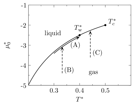
Figure 1: Bulk phase diagram $\mu_{0,co}(T)$ of liquid-gas coexistence according to Eq. (24) in the $\mu^{*}_{0}-T^{*}$ plane for the salt-free ($I=0$) case of a pure solvent. If the wetting transition temperature $T^{*}_{\text{w}}$ is above the triple point $T^{*}_{t}\simeq 0.21$ (for water), three types of paths (A), (B), and (C) are used to study the wetting behavior of our model. (A) is a path along gas-liquid coexistence on the gas side whereas along the paths (B) and (C) two-phase coexistence is approached along isotherms leading to incomplete (B) and complete (C) wetting, respectively.

For a given ionic strength $I=\rho_{\pm}^{(\mathrm{l})}$ in the liquid phase of the solution, the liquid-gas coexistence curves, i.e., the solvent density in the liquid phase of the solution and the coexisting densities of the ions and of the solvent in the gas phase of the solution, are determined by the equality of the chemical potentials $\mu_{0}$ and $\mu_{I}$ and of the pressure $p$:

$$\mu_{0}[\{\rho_{i}^{(g)}\},T^{*}] =\mu_{0}[\{\rho_{i}^{(\mathrm{l})}\},T^{*}],$$ (26)

$$\mu_{I}[\{\rho_{i}^{(g)}\},T^{*}] =\mu_{I}[\{\rho_{i}^{(\mathrm{l})}\},T^{*}],$$

$$p[\{\rho_{i}^{(g)}\},T^{*}] =p[\{\rho_{i}^{(\mathrm{l})}\},T^{*}].$$

For $I=0$ the resulting phase diagram can be determined analytically and is plotted in Fig. 1. The reduced critical temperature is $T^{*}_{c}(I=0)=0.5$ and the critical number density is $\rho_{0,c}(I=0)=0.5$. For $I\neq 0$ the binodal curves are determined numerically and the critical points are obtained by determining the maximum of the corresponding spinodal curves. Within the present model the reduced critical temperature $T^{*}_{c}$ is independent of $I$ whereas $\rho_{0,c}(I)=0.5-2I$. In agreement with experimental evidence Seah1993 the shift of the binodal curves is negligibly small for ionic strengths up to 10 mM, i.e., $I\leq 3.9\times 10^{-4}$.

III.2 Wetting

III.2.1 Salt-free solvent

We first consider the case $I=0$, in which our model reduces to the lattice-gas model studied by Pandit et al. Pandit1982 ; Pandit1983 . In that case, the Euler-Lagrange equations in Eq. (19) reduce to

$$\ln{\rho_{0}(\bar{z})}-\ln{[1-\rho_{0}(\bar{z})]}-\mu^{*}_{0}-\beta u_{\text{w}}\delta_{1,\bar{z}}\\ -\frac{1}{3T^{*}}\left[4\rho(\bar{z})+\rho(\bar{z}+1)+\rho(\bar{z}-1)\right]=0,$$ (27)

and the ratio $u_{\text{w}}/u=3T^{*}\beta u_{w}$ controls the wetting and drying transitions. For $u_{\text{w}}/u>1$ the substrate is so strong that it is already wet at $T^{*}=0$; in the range $0.5<u_{\text{w}}/u<1$ there is a wetting transition at $T^{*}_{\text{w}}>0$; and in the parameter range $0\leq u_{\text{w}}/u<0.5$ a drying transition occurs. Depending on the value of the ratio $u_{\text{w}}/u$ one observes layering transitions, i.e., one can distinguish the number of discrete layers which are forming upon reaching thick films. The transition from $n$ to $n+1$ layers is first order and shows up as a jump in the film thickness $l$. The loci of these discontinuities are layering transition lines, each ending at a critical point $T^{*}_{c,n}$. For large $n$, $T^{*}_{c,n}$ approaches the roughening transition. However, within the present mean-field theory $T^{*}_{c,n}$ approaches $T^{*}_{c}$. Since layering transitions should only occur along or near the melting curve or the sublimation line, these layering transitions are a special feature of the lattice-gas model used to describe the liquid and gas phases Dietrich1988 .

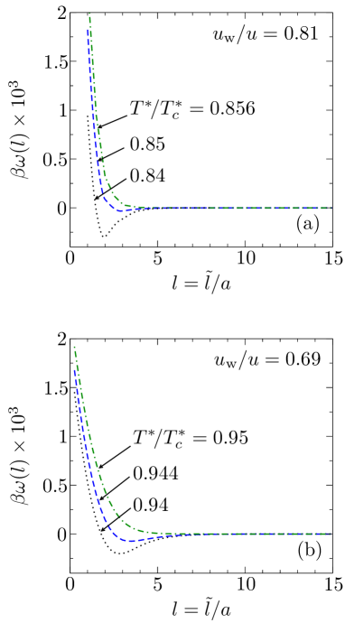
Figure 2: Effective interface potential $\omega(l)=\Omega_{s}(l)-\gamma_{g,l}-\gamma_{l,s}$ at two-phase coexistence as a function of the thickness $\tilde{l}=la$ of the adsorbed liquid film for three temperatures in the salt-free case ($I=0$) for $u_{\text{w}}/u=0.81$ (a) and $u_{\text{w}}/u=0.69$ (b) . In both cases $\omega(l)$ exhibits only a single minimum, the position of which diverges continuously as $T^{*}\to T^{*}_{\text{w}}$. Accordingly, the system undergoes critical wetting at $T^{*}_{\text{w}}\simeq 0.856T^{*}_{c}$ for $u_{\text{w}}/u=0.81$ and at $T^{*}_{\text{w}}\simeq 0.95T^{*}_{c}$ for $u_{\text{w}}/u=0.69$.

We have carried out calculations in the parameter range $0.5<u_{\text{w}}/u<1$. A wider range of the parameter $u_{\text{w}}/u$ was studied thoroughly by Pandit et al. Pandit1982 ; Pandit1983 . Figure 2 shows the effective interface potential $\omega(l)=\Omega_{s}(l)-\gamma_{g,l}-\gamma_{l,s}$ for three different temperatures along a path at coexistence [path (A) in Fig. 1] for the rather arbitrarily chosen values $u_{\text{w}}/u=0.81$ and $u_{\text{w}}/u=0.69$. Here $\gamma_{g,l}$ and $\gamma_{l,s}$ are the gas-liquid and liquid-substrate interfacial tensions, respectively, such that by construction at two-phase coexistence $\omega(l\to\infty)=0$. The equilibrium thickness of the liquid film is given by the position of the global minimum of $\omega(l)$. If $l=\infty$ is the global minimum of $\Omega_{s}(l)$ the system is wet. In this case, the gas-substrate surface tension is given by $\gamma_{g,s}=\Omega_{s}(l=\infty)=\gamma_{g,l}+\gamma_{l,s}$.

In the two cases which we have considered in Fig. 2, $\omega(l)$ exhibits only a single minimum, the position of which diverges continuously or via steps of finite size as $T^{*}\to T^{*}_{\text{w}}$. For $T^{*}>T^{*}_{\text{w}}$ the position of the minimum is $l=\infty$ and the system is wet. The wetting transition is second order and occurs at the temperature $T^{*}_{\text{w}}\simeq 0.856T^{*}_{c}$ for $u_{\text{w}}/u=0.81$ and at $T^{*}_{\text{w}}\simeq 0.95T^{*}_{c}$ for $u_{\text{w}}/u=0.69$. Within the present model, in which all interactions are of the nearest-neighbor type only for the pure solvent, the system exhibits a second-order wetting transition in the entire parameter range $0.5<u_{\text{w}}/u<1$. This observation is compatible with corresponding Monte Carlo simulations of the Ising model on a cubic lattice Binder1988 ; Binder1989 . However, the order of wetting transitions depends sensitively on the range of interactions as well as on whether a continuous or a lattice model is considered. For a continuous analogue of the present model, Pandit et al. Pandit1983 found a second-order wetting transition only for $0.5<u_{\text{w}}/u\lesssim 0.7$ but a first-order one for $u_{\text{w}}/u\gtrsim 0.7$.

Moreover, lattice-gas models with short-ranged particle-particle interactions and long-ranged substrate potentials were studied by de Oliveira and Griffiths Oliveira1978 and Ebner Ebner1980 ; Ebner1981 . In Ref. Oliveira1978 complete wetting in a system with $T_{\text{w}}=0$ was studied within mean field theory. Ebner reported $T_{\text{w}}=0$ or a first-order wetting transition depending on the strength of the substrate potential Ebner1980 and studied the same interaction potentials as the ones used in Refs. Oliveira1978 ; Ebner1980 applying Monte Carlo simulations Ebner1981 . Finally, in systems in which both the particle-particle interactions and the substrate potentials are long-ranged, critical (i.e., second-order) and first-order wetting can occur for suitable choices of the interaction potentials Dietrich1985 ; Ebner1985 .

The film thickness $l=\tilde{l}/a$ as function of $\mu^{*}_{0,co}(T^{*})-\mu^{*}_{0}$, when bulk coexistence $\mu_{0,co}(T^{*})$ (see Fig. 1) is approached along four isotherms from the gas phase [paths of type (B) and (C) in Fig. 1], is plotted in Fig. 3. In the case $u_{\text{w}}/u=0.81$ (Fig. 3(a)) the isotherms exhibit vertical steps at the aforementioned layering transitions. Above $T^{*}_{\text{w}}$, i.e., when the substrate is completely wet at coexistence, the isotherms exhibit an unlimited number of such steps as $\mu^{*}_{0,co}(T^{*})-\mu^{*}_{0}$ approaches zero, while for $T^{*}<T^{*}_{\text{w}}$ there is only a finite number of steps. For $u_{\text{w}}/u=0.69$ (Fig. 3(b)) layering transitions do not occur and the film thickness diverges logarithmically for $T^{*}>T^{*}_{\text{w}}$, while for $T^{*}<T^{*}_{\text{w}}$ it reaches a finite value at coexistence.

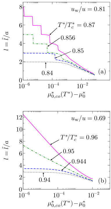
Figure 3: Film thickness $l=\tilde{l}/a$ in units of the lattice constant $a$ as a function of undersaturation $\mu^{*}_{0,co}(T^{*})\!-\!\mu^{*}_{0}$ for the salt-free case ($I=0$). Gas-liquid coexistence $\mu^{*}_{0,co}(T^{*})$ is approached from the gas phase. (a) $u_{\text{w}}/u=0.81$: for $T^{*}<T^{*}_{\text{w}}=0.856T^{*}_{c}$ the system is partially wet and, if at all, there is a finite number of layering transitions; for $T^{*}>T^{*}_{\text{w}}$ the isotherms exhibit an unlimited number of layering transitions as $\mu^{*}_{0,co}(T^{*})\!-\!\mu^{*}_{0}\to 0$ and the first few layering transitions are rounded because for this temperature $T^{*}>T^{*}_{c,n}$. (b) $u_{\text{w}}/u=0.69$: the film thickness diverges logarithmically for $T^{*}>T^{*}_{\text{w}}=0.95T^{*}_{c}$, while it reaches a finite value at coexistence for $T^{*}<T^{*}_{\text{w}}$. In (b) there are no layering transitions. Note that with $T^{*}_{c}(I)=\frac{1}{2}$ one has $\mu^{*}_{0,co}(T^{*})\!-\!\mu^{*}_{0}=\frac{2/3}{T^{*}/T^{*}_{c}}\left[\frac{\mu_{0,co}(T^{*})-\mu_{0}}{u}\right]$.

III.2.2 Electrolyte solution

Within the above concepts we now focus on the influence of the ionic strength $\tilde{I}=Ia^{-3}$ and of the surface charge density $\tilde{\sigma}=\sigma ea^{-2}$ on the wetting behavior of systems with $u_{\text{w}}/u=0.81$ or $u_{\text{w}}/u=0.69$. If the substrate is neutral ($\sigma=0$), the addition of salt changes neither the order nor the transition temperature of the wetting transition, i.e., there is a second-order wetting transition at the wetting temperature $T^{*}_{\text{w}}$ as discussed in the previous Subsubsec. III.2.1. This is expected because within our model all particles have the same size, the ions have the same absolute charge, and the strength of the particle-particle and of the substrate-particle nearest-neighbor interactions are the same for all three species. Hence local charge neutrality ($\rho_{+}(\bar{z})=\rho_{-}(\bar{z})$) holds due to the exchange symmetry with respect to the ionic components. This implies that there is no electric field ($D(\bar{z})=0$). If the surface charge becomes non-zero, the order of the wetting transition changes from second order ($\sigma=0$) to first order ($\sigma\neq 0$) for all values of the charge density $\sigma$ and ionic strength $I$ studied here, with $\sigma=2\times 10^{-5}\ (\text{i.e.,\ }\tilde{\sigma}\approx 0.002~{}\mu\text{C}/\text{cm}^{2})$ as the smallest non-zero value considered. This result is in agreement with previous studies. The influence of ionic solutes on the order of the wetting transition was studied in Ref. Denesyuk2004 by using Cahn’s phenomenological theory and in Ref. Oleksy2009 by using density functional theory for an explicit solvent model for an ionic solution. Both studies suggest that electrostatic interactions favor first-order wetting.

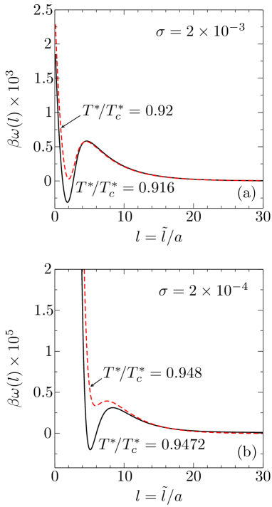
Figure 4: Effective interface potential $\omega(l)$ at gas-liquid coexistence as function of the thickness $l=\tilde{l}/a$ of the liquid film for $u_{\text{w}}/u=0.69$, $I=3.9\times 10^{-5}$ ($\tilde{I}=1$mM), and $\sigma=2\times 10^{-3}$ ($\tilde{\sigma}=0.2\mu\text{C/cm}^{2}$) in (a) and $\sigma=2\times 10^{-4}$ ($\tilde{\sigma}=0.02\mu\text{C/cm}^{2}$) in (b) for two temperatures in each case. The effective interface potential $\omega(l)$ has two local minima (one at $l<\infty$ and one at $l=\infty$) which have the same depth at $T^{*}_{\text{w}}$. Accordingly, for both surface charge densities $\sigma$ the system undergoes a first-order wetting transition.

Figure 4 shows examples of the effective interface potential $\omega(l)$ in the case of non-zero surface charge densities, $\sigma=2\times 10^{-3}$ and $\sigma=2\times 10^{-4}$, for two temperatures and at bulk coexistence [see path (A) in Fig. 1]. In both cases, $\omega(l)$ has two local minima. For $T^{*}<T^{*}_{\text{w}}$ the global minimum corresponds to a thin film whereas for $T^{*}>T^{*}_{\text{w}}$ the film is macroscopically thick. At the wetting transition temperature $T^{*}_{\text{w}}$ the two minima correspond to the same value of the effective interface potential $\omega(l)$. Accordingly, at $T^{*}_{\text{w}}$ the film thickness jumps discontinuously from a finite value below $T^{*}_{\text{w}}$ to a macroscopic one above $T^{*}_{\text{w}}$  so that the system undergoes a first-order wetting transition. If $\sigma$ is decreased the height of the barrier in $\omega(l)$ at the wetting temperature $T^{*}_{\text{w}}$ decreases and the minimum close to the wall is shifted to larger thicknesses (Fig. 4(b)). In the case $\sigma=0$, $\omega(l)$ has only a single minimum, like in the salt-free case (see Fig.  2), corresponding to a second-order wetting transition.

In Fig. 5 the wetting transition temperature is plotted as function of the surface charge density for two values of the ionic strength and for $u_{\text{w}}/u=0.81$. As $\sigma=\tilde{\sigma}a^{2}/e$ is increased, the wetting transition temperature $T^{*}_{\text{w}}$ decreases due to the strengthening of the substrate-fluid attraction as the substrate is charged up. For $\sigma\neq 0$ the system with a smaller ionic strength $I$ has always the lower wetting transition temperature $T^{*}_{\text{w}}$ because in this case the screening of the electrostatic forces of the substrate is reduced making them effectively stronger which favors wetting. As already mentioned above, within our model for $\sigma=0$ the wetting transition temperature is independent of the ionic strength $\tilde{I}=Ia^{-3}$. The trend is the same for $u_{\text{w}}/u=0.69$. In the case of first-order wetting transitions these results are in qualitative agreement with Ref. Oleksy2009 . However, the off-lattice model used therein exhibits also second-order wetting transitions (see the discussion above in Subsubsec. III.2.1), for which $T^{*}_{\text{w}}$ is a non-monotonic function of $\sigma$.

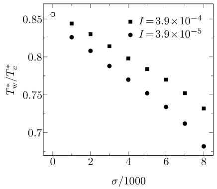
Figure 5: Wetting transition temperature $T^{*}_{\text{w}}$ as a function of the substrate surface charge density $\sigma=\tilde{\sigma}a^{2}/e$ for $u_{\text{w}}/u=0.81$. The two types of symbols correspond to distinct values of the ionic strength $I=\tilde{I}a^{3}$ in the bulk liquid phase ($\bullet$ for $I=3.9\times 10^{-5}$ ($\tilde{I}=1$mM) and $\blacksquare$ for $I=3.9\times 10^{-4}$ ($\tilde{I}=10$mM)). Filled symbols correspond to first-order wetting transitions, while the empty one at $\sigma=0$ corresponds to a second-order wetting transition, with the corresponding wetting transition temperature being independent of $I$.

Since the wetting transitions for $\sigma\neq 0$ are first order, there is a prewetting line associated with them. The prewetting line is attached tangentially to the gas-liquid coexistence line at the wetting temperature $T^{*}_{\text{w}}$ and bends away from coexistence, marking the loci of a finite discontinuity in film thickness $l=\tilde{l}/a$. The discontinuity upon crossing the prewetting line gets smaller as one moves further away from coexistence and it vanishes at the prewetting critical point. Figure 6 shows the film thickness $l=\tilde{l}/a$ for four different isotherms as a function of undersaturation $\mu^{*}_{0,co}(T^{*})-\mu^{*}_{0}$ for $u_{\text{w}}/u=0.81$ and $\sigma=2\times 10^{-3}$ ($\tilde{\sigma}=0.2\mu\text{C}/\text{cm}^{2}$). The film thickness increases for small undersaturation as $l\sim\ln(\mu^{*}_{0,co}(T^{*})-\mu^{*}_{0})$. Accordingly, $\omega(l)\sim\exp(-2\kappa l)$, where $\kappa=\sqrt{8\pi l_{B}I/\varepsilon(\rho_{0}^{\mathrm{l}})}$ is the inverse Debye length (see inset of Fig. 6). This is in agreement with Refs. Kayser1988 and Denesyuk2004 for wetting of solvents with added salt. In contrast, for wetting films of solvents without addition of salt, i.e., with counterions only, one has $l\sim(\mu_{co}-\mu)^{-1/2}$ and $\omega(l)\sim l^{-1}$ Langmuir1938 ; Kayser1986 ; Denesyuk2004 ; Derjaguin1974 . In order to obtain this result, Eqs. (2) and (10) have to be modified to consider only solvent particles and counterions but leaving out coions. In addition to the finite thin-thick jumps in film thickness $l$ when crossing the prewetting line we observe first-order layering transitions similar to those found in the salt-free case for $u_{\text{w}}/u=0.81$ (see Fig. 3). The addition of the electrostatic interaction leads to a series of triple points where the layering transition lines meet the prewetting line, as shown in the surface phase diagram in Fig. 7. A similar phase diagram was found by Ebner Ebner1980 using a lattice-gas model for a one-component fluid in which the fluid particles interact among each other via a Lennard-Jones (6-12) potential and a fluid particle interacts with the substrate via a (9-3) potential. This is also in line with the prediction by Pandit et al. Pandit1982 for a substrate of intermediate strength, i.e., for $0.5<u_{\text{w}}/u<1$, with interactions ranging beyond nearest neighbors.

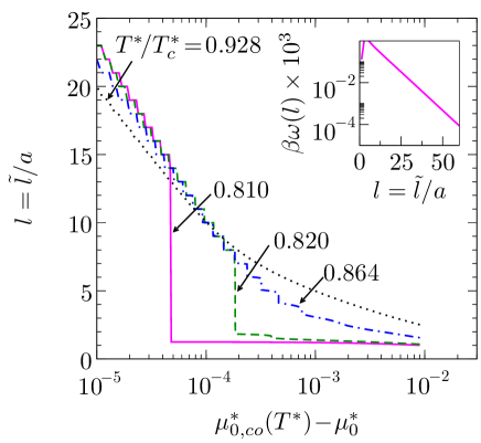
Figure 6: The film thickness $l=\tilde{l}a$ (Eq. (22)) as a function of undersaturation $\mu^{*}_{0,co}(T^{*})\!-\!\mu^{*}_{0}$ along four different isotherms for $u_{\text{w}}/u=0.81$, $I=3.9\times 10^{-5}$ ($\tilde{I}=1$mM), and $\sigma=2\times 10^{-3}$ ($\tilde{\sigma}=0.2\mu\text{C}/\text{cm}^{2}$) exhibits a large but finite jump (corresponding to more than one monolayer) when the prewetting line is crossed and small jumps when the various layering transition lines are crossed. The film thickness increases for small undersaturation as $l\sim\ln(\mu^{*}_{0,co}(T^{*})\!-\!\mu^{*}_{0})$ where $\mu^{*}_{0,co}(T^{*})\!-\!\mu^{*}_{0}=\tfrac{2/3}{T^{*}/T^{*}_{c}}\left[\tfrac{\mu_{0,co}(T^{*})-\mu_{0}}{u}\right]$. The inset displays the corresponding asymptotic behavior of the effective interface potential $\omega(l)\sim\exp(-2\kappa l)$ where $\kappa=\sqrt{8\pi l_{B}I/(\varepsilon(\rho_{0}^{(\mathrm{l})})}$ is the inverse Debye length.

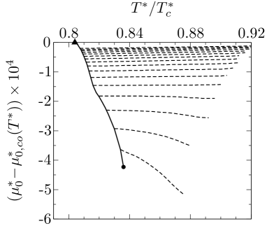
Figure 7: Surface phase diagram for $u_{\text{w}}/u=0.81$ and $\sigma=2\times 10^{-3}$ ($\tilde{\sigma}=0.2\mu\text{C}/\text{cm}^{2}$) . The full line is the prewetting line attached to $T_{\text{w}}^{*}=0.864\,T^{*}_{c}$ ($\blacktriangle$) and ending at the prewetting critical point ($\bullet$). The dashed lines correspond to layering transition lines. They end at layering critical points $T^{*}_{c,n}$ (located at the end of the dashed lines without being indicated separately), which within the present mean-field theory accumulate for $n\to\infty$ at $T^{*}_{c}$ instead of at the roughening transition temperature of the gas-liquid interface on the lattice.

In the case $u_{\text{w}}/u=0.81$ and for fixed ionic strength $I$ we have studied the prewetting lines for various values of the surface charge density $\sigma$. Figure 8 shows the prewetting lines for ionic strength $I=3.9\times 10^{-5}$ ($\tilde{I}=1$mM) and for four values of $\sigma$. One can see clearly that as $\sigma$ decreases, the wetting temperature $T^{*}_{\text{w}}$ rises and the prewetting line becomes shorter. This is in agreement with the fact that in the limit $\sigma\to 0$ the wetting transition turns second order. The values of the prewetting critical points for the lines shown in Fig. 8 are given in Table 1.

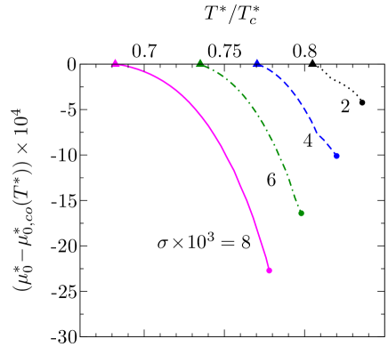
Figure 8: Prewetting lines for four values of the surface charge density $\sigma=\tilde{\sigma}a^{2}/e$ with ionic strength $I=3.9\times 10^{-5}$ ($\tilde{I}=1$mM) in the bulk liquid phase and for $u_{\text{w}}/u=0.81$. The locations of the wetting transitions ($\blacktriangle$) and of the prewetting critical points ($\bullet$) are given in Table 1.

$\sigma=\tilde{\sigma}a^{2}/e$	$T^{*}_{\text{w}}/T^{*}_{c}$	$T^{*}_{p\text{w},c}/T^{*}_{c}$	$\mu^{*}_{0,co}\left(T^{*}_{p\text{w},c}\right)-\mu^{*}_{0,p\text{w},c}$
$2\times 10^{-3}$	0.804	0.836	$4.23\times 10^{-4}$
$4\times 10^{-3}$	0.77	0.82	$1.01\times 10^{-3}$
$6\times 10^{-3}$	0.734	0.798	$1.60\times 10^{-3}$
$8\times 10^{-3}$	0.682	0.778	$2.27\times 10^{-3}$

Table 1: Prewetting critical points $(T^{*}_{p\text{w},c},\mu^{*}_{0,p\text{w},c})$ for the prewetting lines shown in Fig. 8. The ionic strength in the liquid phase is $I=3.9\times 10^{-5}$ ($\tilde{I}=1$mM). $T^{*}_{\text{w}}$ is the transition temperature for first-order wetting. Note that $\mu^{*}_{0,co}(T^{*}_{p\text{w},c})\!-\!\mu^{*}_{0,p\text{w},c}=\tfrac{2/3}{T^{*}_{p\text{w},c}/T^{*}_{c}}\left[\tfrac{\mu_{0,co}(T^{*}_{p\text{w},c})-\mu_{0,p\text{w},c}}{u}\right]$.

IV Conclusions and Summary

We have investigated wetting of a charged substrate by an electrolyte solution with a focus on the influence of the ionic strength $I$ and of the substrate surface charge $\sigma$ on the wetting behavior. First, we have investigated a lattice-gas model for the salt-free, i.e., pure solvent (Fig. 1) providing a reference system relative to which the influence of the electrostatic interaction can be compared. The results for the salt-free case are in good agreement with previous studies Pandit1983 ; Pandit1982 . We have calculated the effective interface potential $\omega(l)$ which facilitates the transparent identification of the order of the wetting transition (see Fig. 2). Depending on the value of the ratio $u_{\text{w}}/u$ of the strengths of the substrate potential and of the particle-particle interaction, the model can exhibit layering transitions when gas-liquid coexistence is approached along an isotherm (see Fig. 3). In the next step we have analyzed quantitatively the effects of the ionic strength and of the surface charge density on the order and on the transition temperature of the wetting transition. Concerning the order of the transition we have found that electrostatic forces induce a first-order wetting transition, even for very small surface charges (see Fig. 4). Within our model, for $\sigma=0$ the transition is second order and occurs at the same temperature as in the salt-free case. For a fixed ionic strength, the wetting temperature $T^{*}_{\text{w}}$ decreases with increasing surface charge density of the substrate. This is due to the increasing substrate-fluid attraction as the substrate surface charge is increased. If systems, which differ only with respect to the ionic strength $I$, are compared, the one with smaller $I$ has the lower wetting transition temperature $T^{*}_{\text{w}}$ (see Fig. 5). When bulk coexistence is approached along an isotherm, in the case of a first-order wetting transition, i.e., if $\sigma\neq 0$, the model exhibits first-order layering transitions in addition to prewetting (Fig. 6). This leads to a series of triple points in the surface phase diagram (see Fig. 7). We have also studied the influence of the surface charge density on the prewetting lines. We have found that the prewetting line becomes shorter as the surface charge density is decreased (Fig. 8).

Although our lattice model differs significantly from the continuum models used in Refs. Denesyuk2004 ; Oleksy2009 , we have arrived at similar conclusions concerning the trend that adding ions promotes first-order wetting transitions. Accordingly, this result can be considered to be robust. Within our approach one is able to study wide interfacial regions and therefore small ionic strengths which was not possible within the model studied in Ref. Oleksy2009 . Our study also includes a discussion of prewetting, providing a more complete description of the wetting properties of electrolytes. In agreement with Refs. Denesyuk2004 ; Kayser1988 the growth law of the film thickness for complete wetting along an isotherm is not changed by adding ions to the solvent, in spite of their long-ranged Coulombic interaction (Figs. 3 and 6) . However, if only counterions are considered, which are donated by the substrate and the charge of which is opposite to that of the wall, the film thickness varies as $l\sim(\mu_{co}-\mu)^{-1/2}$ Langmuir1938 ; Kayser1986 ; Denesyuk2004 .

References

- (1) P. G. de Gennes, Rev. Mod. Phys. 57, 827 (1985).
- (2) S. Dietrich, in Phase Transitions and Critical Phenomena, edited by C. Domb and J. L. Lebowitz, (Academic, London, 1988), Vol. 12, p. 1.
- (3) M. Schick, in Liquids at interfaces, edited by J. Charvolin, J. F. Joanny, and J. Zinn-Justin (North-Holland, Amsterdam, 1988), p. 415
- (4) D. Bonn and D. Ross, Rep. Prog. Phys. 64, 1085 (2001).
- (5) D. Bonn, J. Eggers, J. Indekeu, J. Meunier, and E. Rolley, Rev. Mod. Phys. 81, 739 (2009).
- (6) F. Mugele and J.-C. Baret, J. Phys.: Condensed Matter 17, R705 (2005).
- (7) D. H. Everett, Basic Principles of Colloid Science, RSC Paperbacks (The Royal Society of Chemistry, London, 1988).
- (8) M. G. Pollack, R. B. Fair, and A. D. Shenderov, Appl. Phys. Lett. 77, 1725 (2000).
- (9) O. D. Velev, B. G. Prevo, and K. H. Bhatt, Nature 426, 515 (2003).
- (10) I. Langmuir, Science 88, 430 (1938).
- (11) A. C. Hall, J. Phys. Chem. 74, 2742 (1970).
- (12) B. Derjaguin and N. Churaev, J. Colloid Interf. Sci. 49, 249 (1974).
- (13) R. F. Kayser, Phys. Rev. Lett. 56, 1831 (1986).
- (14) R. Kayser, J. Phys. (France) 49, 1027 (1988).
- (15) N. A. Denesyuk and J.-P. Hansen, J. Chem. Phys. 121, 3613 (2004).
- (16) A. Oleksy and J.-P. Hansen, Mol. Phys. 107, 2609 (2009).
- (17) A. Oleksy and J.-P. Hansen, J. Chem. Phys. 132, 204702 (2010).
- (18) Y. Rosenfeld, J. Chem. Phys. 89, 4272 (1988).
- (19) Y. Rosenfeld, Phys. Rev. Lett. 63, 980 (1989).
- (20) G. Torrie and J. Valleau, Chem. Phys. Lett. 65, 343 (1979).
- (21) J. D. Jackson, Classical Electrodynamics, 3rd ed. (Wiley, New York, 1999).
- (22) M. S. Wertheim, J. Chem. Phys. 55, 4291 (1971).
- (23) S. L. Carnie and D. Y. C. Chan, J. Chem. Phys. 73, 2949 (1980).
- (24) J. L. Lebowitz and E. H. Lieb, Phys. Rev. Lett. 22, 631 (1969).
- (25) E. H. Lieb and J. L. Lebowitz, Adv. Math. 9, 316 (1972)
- (26) Z. Xu, Phys. Rev. E 87, 013307 (2013).
- (27) R. Evans, Adv. Phys. 28, 143 (1979).
- (28) M. Bellac, Quantum and Statistical Field Theory (Oxford Science Publications, 1991).
- (29) M. Plischke and B. Bergersen, Equilibrium Statistical Physics, 2nd ed. (World Scientific, Singapore, 2006).
- (30) P. M. Chaikin and T. Lubensky, Principles of Condensed Matter Physics (Cambridge University Press, 2000).
- (31) S. A. Safran, Statistical Thermodynamics of Surfaces, Interfaces, and Membranes (Westview, Boulder, 2003).
- (32) M. Bier, A. Gambassi, and S. Dietrich, J. Chem. Phys. 137, 034504 (2012).
- (33) J. Sonnefeld, Colloids Surf. A 108, 27 (1996).
- (34) C. Seah, C. A. Grattoni, and R. A. Dawe, Fluid Phase Equilib. 89, 345 (1993).
- (35) R. Pandit, Phys. Rev. B 26, 5112 (1982).
- (36) R. Pandit and M. Wortis, Phys. Rev. B 25, 3226 (1982).
- (37) K. Binder and D. P. Landau, Phys. Rev. B 37, 1745 (1988).
- (38) K. Binder, D. P. Landau, and S. Wansleben, Phys. Rev. B 40, 6971 (1989).
- (39) M. D. Oliveira and R. B. Griffiths, Surf. Sci. 71, 687 (1978).
- (40) C. Ebner, Phys. Rev. A 22, 2776 (1980).
- (41) C. Ebner, Phys. Rev. A 23, 1925 (1981).
- (42) S. Dietrich and M. Schick, Phys. Rev. B 31, 4718 (1985).
- (43) C. Ebner, W. F. Saam, and A. K. Sen, Phys. Rev. B 31, 6134 (1985).