Orbital anisotropy in cosmological haloes revisited

Abstract

The velocity anisotropy of particles inside dark matter (DM) haloes is an important physical quantity, which is required for the accurate modelling of mass profiles of galaxies and clusters of galaxies. It is typically measured using the ratio of the radial-to-tangential velocity dispersions at a given distance from the halo centre. However, this measure is insufficient to describe the dynamics of realistic haloes, which are not spherical and are typically quite elongated. Studying the velocity distribution in massive DM haloes in cosmological simulations, we find that in the inner parts of the haloes the local velocity ellipsoids are strongly aligned with the major axis of the halo, the alignment being stronger for more relaxed haloes. In the outer regions of the haloes, the alignment becomes gradually weaker and the orientation is more random. These two distinct regions of different degree of the alignment coincide with two characteristic regimes of the DM density profile: a shallow inner cusp and a steep outer profile that are separated by a characteristic radius at which the density declines as $\rho\propto r^{-2}$. This alignment of the local velocity ellipsoids requires reinterpretation of features found in measurements based on the spherically averaged ratio of the radial-to-tangential velocity dispersions. In particular, we show that the velocity distribution in the central halo regions is highly anisotropic. For cluster-size haloes with mass $10^{14}-10^{15}{{h^{-1}{\rm{M_{\odot}}}}}$, the velocity anisotropy along the major axis is nearly independent of radius and is equal to $\beta=1-\sigma^{2}_{\rm perp}/\sigma^{2}_{\rm radial}\approx 0.4$, which is significantly larger than the previously estimated spherically averaged velocity anisotropy. The alignment of density and velocity anisotropies, and the radial trends may also have some implications for the mass modelling based on kinematical data of such objects as galaxy clusters or dwarf spheroidals, where the orbital anisotropy is a key element in an unbiased mass inference.

1 Introduction

The orbital anisotropy describes the distribution of orbits in astrophysical systems. It plays a key role in dynamical modelling of kinematical data of objects at all scales, from the stellar halo of the Milky Way (Kafle et al., 2012), dwarf spheroidals (Łokas, 2009; Walker et al., 2009), to elliptical galaxies (Dekel et al., 2005; Napolitano et al., 2011; Wojtak & Mamon, 2012) and galaxy clusters (Biviano & Girardi, 2003; Wojtak & Łokas, 2010). Prior knowledge on the anisotropy or elaborated techniques of data analysis are essential for accurate and unbiased mass estimates. The main difficulty arises from the well-known mass-anisotropy degeneracy occurring in the Jeans analysis of the velocity dispersion profiles (Merritt, 1987). Several methods were developed to break this degeneracy (see e.g. Łokas, 2002; Łokas & Mamon, 2003; Wojtak et al., 2009; Wolf et al., 2010; Mamon et al., 2012). Their efficiency, however, critically relies on the quality of the data. In addition, observational constraints on the mass profiles are still affected by what dynamical models assume about the anisotropy or what priors on the anisotropy are used. As the matter of fact, most models rely on certain parametrisation of the anisotropy (e.g. Łokas, 2002; Mamon et al., 2012; Wojtak et al., 2009) or incorporate some well-motivated profiles (e.g. Diaferio, 1999; Dekel et al., 2005) or prior distributions for its parameters (e.g. Newman et al., 2012). The choice of the prior probability and parametrisation is commonly motivated by cosmological $N$-body simulations. The orbital anisotropy in DM haloes is often used as a point of reference in such preselection of dynamical models. The best example showing this effect of feedback from the simulations is the commonly adopted assumption that the velocity distribution in the centre of gravitationally bound cosmological objects is isotropic or nearly isotropic (see e.g. Walker et al., 2006; Newman et al., 2012, as examples in studies of dwarf spheroidals and galaxy clusters).

The orbital anisotropy is also a quantity of great interest in the context of studying velocity distributions of DM particles in simulated haloes. Many studies showed a number of interesting properties such as a relation between the anisotropy and DM density profile (Hansen & Moore, 2006; Zait et al., 2008) or existence of a universal attractor in the space spanned by all solutions of the Jeans equation (Hansen et al., 2010). The anisotropy parameter is often a part of equilibrium models describing DM haloes (see e.g. Dehnen & McLaughlin, 2005), though recent studies showed that it is not relevant in mapping between the mass and the phase-space density profiles (Ludlow et al., 2011). A number of studies addressed such problems as the radial profiles of the anisotropy (Wojtak et al., 2005; Ascasibar & Gottlöber, 2008), the bias between DM particles and subhaloes (Diemand et al., 2004), evolution of the anisotropy in controlled simulations of halo mergers (Sparre & Hansen, 2012), the redshift evolution (Iannuzzi & Dolag, 2012) and dependance on the mass and dynamical equilibrium of DM haloes (Lemze et al., 2012). The overall picture emerging from these studies points to the fact that the velocity distribution is nearly isotropic in the halo centre and radially biased at large radii (excess of radial orbits). Although this trend is common to all DM haloes, the anisotropy profiles of individual haloes are significantly scattered around the mean trend. Deviation from the mean trend seems to depend on dynamical stage of the haloes (Lemze et al., 2012).

The global velocity ellipsoids of DM haloes are aligned with the major axes of the halo shape (Kasun & Evrard, 2005; Allgood et al., 2006; Saro et al., 2012). This property seems to occur also locally, although this problem has not been extensively studied in the literature (Zemp et al., 2009). Interestingly, similar configuration of the velocity ellipsoid is consistent with the kinematical data of elliptical galaxies (Cappellari et al., 2007) and galaxy clusters (Skielboe et al., 2012) what suggests that it is probably a generic feature of the orbital structure in cosmological objects. Despite these facts, the orbital anisotropy in simulated DM haloes is commonly quantified in terms of the ratio of the radial-to-tangential velocity dispersions which breaks the preferred symmetry of the velocity distributions. This raises the question to what extent the orbital anisotropy defined in this way describes the true distribution of orbits in DM haloes.

The anisotropy of the velocity dispersion tensor is commonly quantified by the anisotropy parameter (Binney & Tremaine, 2008)

$$\beta=1-\frac{\sigma_{t}^{2}}{2\sigma_{r}^{2}},$$ (1)

where $\sigma^{2}_{\rm r}$ and $\sigma^{2}_{\rm t}$ are the radial and tangential velocity dispersions, respectively. This is a reasonable definition for a spherical or almost spherical halo because in this case the velocity dispersion tensor should be oriented along the radial direction and, because of the symmetry, one expects that dispersions perpendicular to the radius are equal: $\sigma^{2}_{\theta}=\sigma^{2}_{\phi}=\sigma^{2}_{t}/2$. For haloes with substantial elongation – and a large fraction of cluster-size haloes are elongated – the velocity ellipsoid is more complex and simple spherically averaged $\beta(r)$ is not enough to describe such systems.

Despite obvious inconsistencies between the spherically averaged $\beta$ and the elongation of DM haloes, the anisotropy parameter $\beta$ is commonly used to study the phase-space properties of DM haloes. In realistic cases one expects that local velocity tensor is neither aligned along radius nor tangential velocity dispersions are equal. To complicate the situation, the velocity dispersions are also expected to depend on all three space coordinates, not just one radius. So, realistic $\beta(\vec{r})$ is a complex entity. To some degree, this justifies using spherically averaged $\beta$. Realistic $\beta(\vec{r})$ is not well studied and, even it were, it would be more difficult to adopt it in dynamical models. Instead, by using spherically averaged $\beta$, one gets a practical tool to build dynamical models with understanding that there is a price for this simplification: one should expect some errors in the models. Here we do not study the errors and focus only on description of the realistic velocity ellipsoids.

In this paper, we study the properties of the velocity ellipsoids in cluster-size DM haloes in high-resolution cosmological simulations. The paper is organised as follows. In section 2, we describe cosmological simulations and the properties of DM haloes used for the analysis. In section 3, we investigate the local values of the anisotropy parameter defined using the radial and tangential velocity dispersions. This gives us insights into dynamical structure of the halo and it shows that anisotropy parameter depends on the position with respect to the halo major axis. This “classical” treatment of the anisotropy parameter neglects the fact that velocity ellipsoid may not be aligned along radius and that it may be triaxial. In section 4, we study the properties of the local velocity dispersion tensor, e.g. alignment, triaxiality and anisotropy, and we show that the local velocity ellipsoids are aligned with the major axis of the halo shape. In section 5, we calculate spherically averaged (measured in spherical shells) profiles of the orbital anisotropy defined in the symmetry consistent with the alignment of the local velocity ellipsoids and compare with the local values. We also show how the anisotropy parameter based on the ratio of the radial-to-tangential velocity dispersions misrepresents the true orbital structure in DM haloes. Section 6 contains discussion and conclusions. In this section, we also provide a simple analytical model for the local velocity ellipsoids measured in DM haloes.

2 Method

2.1 Simulations

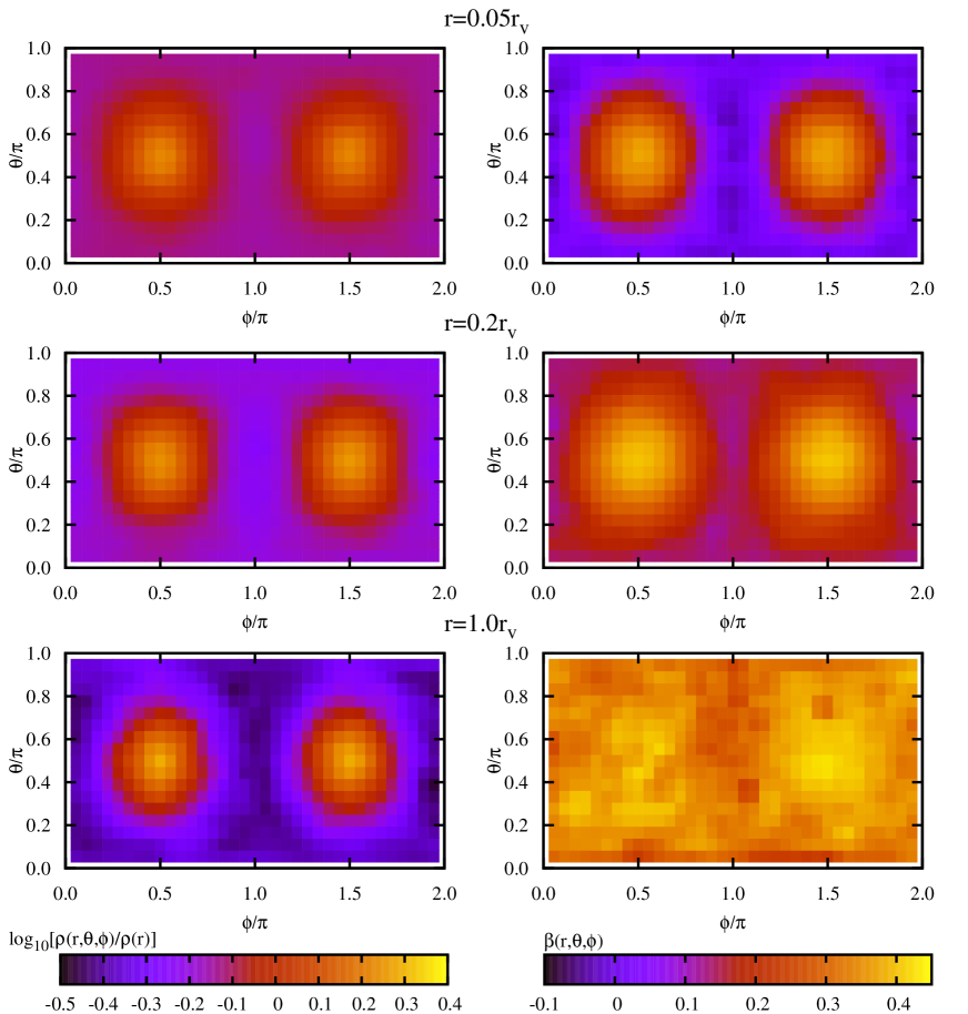
Figure 1: Density and velocity anisotropy of DM haloes as a function of the polar and azimuthal angles $\theta$ and $\phi$. The system of coordinates is chosen in such a way that the major axis is placed at $\theta=\pi/2$ and $\phi=\pi\pm\pi/2$. Left panels: Deviations of the local density from the average density at given radius $\rho(r,\theta,\phi)/\rho(r)$. Right panels: Local velocity anisotropy parameter $\beta$. The rows show the maps calculated inside three spherical shells of radii equal to $0.05$, $0.20$ and $1.00$ of the virial radius. When measured in spherical shells the density anisotropy declines with decreasing radius. However, the pattern of elongation along the major axis is clearly preserved at all radii. The velocity anisotropy $\beta(r,\theta,\phi)$ behaves very differently as compared with the density $\rho(r,\theta,\phi)$. Close to the virial radius the velocities are predominantly radial in all directions: $\beta\approx 0.4$. At smaller distances $\beta$ has same value $\sim 0.4$ along the major axis and gets to $\beta\mathrel{\hbox{\hbox to0.0pt{\hbox{\lower 4.0pt\hbox{$\sim$}}\hss}\hbox{$<$}}}0$ in the plain perpendicular to the major axis.

We use cluster-size DM haloes selected from the Bolshoi simulation (Klypin et al., 2011). The simulation follows the evolution of DM structures in the framework defined by a $\Lambda$CDM cosmological model with cosmological parameters consistent with recent measurements based on WMAP five-year data release (Komatsu et al., 2009) and abundance of the Sloan Digital Sky Survey clusters (Rozo et al., 2010). The simulation box has a side length equal to $250{{h^{-1}{\rm Mpc}}}$ and contains $2048^{3}$ particles, each with mass of $1.35\times 10^{8}{{h^{-1}{\rm{M_{\odot}}}}}$. High mass resolution of the simulation is a key feature to study the properties of the local velocity distributions in DM haloes. For all details on the simulations, we refer the reader to Klypin et al. (2011).

DM haloes are found using the Bound-Density-Maxima (BDM) algorithm (Klypin & Holtzman, 1997). BDM finds all density maxima with density estimated with the top-hat filter containing 20 particles. Among all density maxima inside a given distinct halo the code finds the one which has the deepest gravitational potential and uses it as the centre of the halo. The halo virial mass $M_{\rm v}$ is defined as a spherical overdensity mass with the mean density $\Delta=3M_{\rm v}/(4\pi r_{\rm v}^{3})=97.2$ times greater than the critical density, where $r_{\rm v}$ is the virial radius. For our study, we select all $517$ haloes with virial masses greater than $7\times 10^{13}{{h^{-1}{\rm{M_{\odot}}}}}$. The selected haloes contain from $5\times 10^{5}$ to $8\times 10^{6}$ particles inside the virial sphere. Velocities of DM particles are corrected for the halo bulk velocities approximated by the mean velocity of the particles inside the virial sphere.

2.2 Halo shapes

We quantify the shape of the haloes in terms of the shape tensor given by

$$I_{i,j}=\sum_{n=1}^{N}r_{i,n}r_{j,n},$$ (2)

where $r_{i,n}$ is $i$-th component of the position vector with respect to the halo centre and the sum is over all particles lying inside the virial sphere. Many authors use the normalised positions in order to minimise effect of substructures or to equalise contribution from the particles at small and large distances. However, as shown by Zemp et al. (2011), this weighting leads to a bias when one measures the global shape of the halo. In this case, assigning equal weights to all particles is recommended.

Eigenvectors of the tensor (2) determine the semi-principle axes of an ellipsoid approximating the halo global shape. Information which is essential for our study is the eigenvector associated with the major axis of the halo shape ellipsoid – the axis minimising the moment of inertia.

In general, the semi-principle axes of the halo shape ellipsoid may depend on radius. Cosmological simulated haloes, however, exhibit strong coherence of orientations of the shape ellipsoids measured at different radii (Jing & Suto, 2002; Bailin & Steinmetz, 2005). This means that the major axis of the global halo shape is a well-defined global axis of symmetry, both in the inner and outer parts of the haloes. We use this axis as a reference axis for studying symmetry of the velocity distributions in the selected haloes.

2.3 Relaxed haloes

In our analysis, we also consider a subsample of relaxed haloes. Our criteria of relaxedness are similar to those proposed by Neto et al. (2007) and are based on three diagnostics of dynamical equilibrium: the offset between the mass centre and the minimum of the potential, the offset between the bulk velocity of the halo and the mean velocity of the most gravitationally bound particles, and the virial ratio. We use BDM halo centres as the positions of the minimum of the potential and BDM bulk velocities as velocities of the most gravitationally bound particles. The virial ratio is estimated using $3\times 10^{3}$ particles randomly drawn from every halo. The gravitational binding energy is computed using direct summation.

We define relaxed haloes as those which satisfy three conditions: the offset of the mass centre less than $0.07r_{v}$ and the virial ratio less than $1.35$. The limits imposed on all diagnostics separate the outliers which populate long tails of the distributions and are associated with unrelaxed haloes. Most unrelaxed haloes ($76$ per cent) are found by the offset of the mass centre. Our selection criteria yield $299$ relaxed haloes ($58$ per cent of the total number).

3 Velocity anisotropy along and perpendicular to the major axis

We start our analysis by investigating the global trends in the velocity anisotropy. Here we ask a simple question: how does $\beta$ change along and perpendicular to the major axis of the density distribution.

We compute the local values of the anisotropy parameter on a regular grid of spherical angles inside spherical shells. The polar $\theta$ and azimuthal $\phi$ angles of the halo major axis are set consistently at the same values in all haloes (for the sake of readability of the plots, we chose $\theta=\pi/2$ and $\phi=\pi\pm\pi/2$). We use three spherical shells of radii $(0.03-0.07)r_{\rm v}$, $(0.16-0.25)r_{\rm v}$ and $(0.93-1.07)r_{\rm v}$ containing on average $3.9\times 10^{4}$, $1.2\times 10^{5}$ and $10^{5}$ particles. The anisotropy parameter is calculated inside the cones with opening angle of $10$ degrees around every point of the regular grid representing a cylindrical map projection of a sphere (the Mercator projection), for every spherical shell. At every grid point, we find the median value of the anisotropy parameter in the halo sample. In all results presented below we show the medial values.

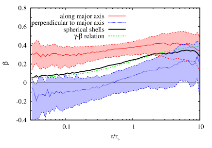
Figure 2: Radial profiles of the anisotropy parameter $\beta$. The profiles are complementary to Figure 1 showing dependance of $\beta$ on the position with respect to the halo major axis. Spherically averaged $\beta(r)$ indicates preferentially radial anisotropy at all radii. It also slightly increases with radius, as found in many studies. Instead, the anisotropy along the density major axis is nearly constant at all radii (with $\beta\approx 0.35$), whereas regions perpendicular to the major axis show tendency to have excess of the tangential velocity dispersion at small distances ($\beta\mathrel{\hbox{\hbox to0.0pt{\hbox{\lower 4.0pt\hbox{$\sim$}}\hss}\hbox{$<$}}}0$). The black dashed line is the linear relation between the anisotropy and the logarithmic density slope from Hansen & Moore (2006). Shaded regions on show $50$ per cent statistical uncertainties.

The right panels of Figure 1 show the dependance of the anisotropy parameter $\beta$ on the position with respect to the halo major axis. The left panels show the values of the ratio $\rho(r,\theta,\phi)/\rho(r)$, where $\rho(r,\theta,\phi)$ is the density inside the intersection of a radial shell and a cone directed to $(\theta,\phi)$, and $\rho(r)$ is the density inside a shell.

The maps of the local anisotropy parameter inside the two inner shells show a dipole-like dependance on the position with respect to the halo major axis. The value of $\beta$ changes from $\approx 0.3$ along the major axis to $\approx 0$ in the plane perpendicular to the major axis. Similar dipole structure, although not as prominent as in the inner shells, is also visible at the virial sphere. Here, the local anisotropy parameter tends to change from $0.5$ (along major axis) to $0.3$ (in the perpendicular plane). We note that the same spatial variation of the local anisotropy parameter has been recently found in non-cosmological controlled simulations of mergers of DM haloes (Sparre & Hansen, 2012). In every shell, the dipole of the anisotropy parameter coincides with the dipole of the density ratio (compare the left and right panels in Figure 1).

The values of the spherically averaged velocity anisotropy (computed in spherical shells) are $0.14$, $0.20$ and $0.30$, from the innermost to outermost shell respectively. One can immediately see that the local values of $\beta$ are substantially larger along the major axis and smaller in the perpendicular plane compared to the spherically averaged values. The local values of $\beta$ in the two innermost shells are consistent with similar measurements obtained by Zemp et al. (2009) from high resolution simulations of a Milky Way size DM halo.

Figure 2 shows the radial profiles of the orbital anisotropy along (up to $30$ degrees from the axis) and perpendicular (up to $\pm 20$ degrees from the plane) to the major axes of the haloes. We scaled radii by the characteristic radius $r_{\rm s}$ where the density profile is proportional to $r^{-2}$. The scale radii $r_{s}$ were obtained from fitting the NFW profile (Navarro et al., 1997) to the density measured in spherical shells of radii equally spaced in logarithmic scale. The quartiles of the anisotropy parameter at each radius were calculated using only these radial bins which lie inside the virial sphere (the mean virial radius of the haloes is equal to $6.2r_{-2}$). The anisotropy along the halo major axes is substantially larger than that the spherically averaged one. Its radial dependance is much weaker then the profile corresponding to the linear relation between the anisotropy and the logarithmic slope of the density profile from Hansen & Moore (2006). The anisotropy in the plane perpendicular to the major axes are substantially smaller and negative and small radii. The profile is consistent with a linear density slope-anisotropy relation with the slope similar to that from (Hansen & Moore, 2006), but different intercept.

Alignment of the velocity anisotropy dipole with the density dipole suggests that the apparent dependance of $\beta$ on the position with respect to the halo major axis may be a purely geometrical effect resulting from a wrong assumption that the local velocity ellipsoids are aligned with the radial directions (assumption underlying the definition of $\beta$). In order to address this problem in more detail, we shall study the properties of the local velocity dispersion tensors.

4 Local velocity ellipsoids

The anisotropy parameter $\beta=1-\sigma_{t}^{2}/(2\sigma_{r}^{2})$ measures the true anisotropy of the velocity distribution only in spherical systems, where one can assume that velocity dispersion tensor is diagonal in spherical coordinate system and two diagonal coefficients are equal: $\sigma_{\theta}^{2}=\sigma_{\phi}^{2}=\sigma_{t}^{2}/2$. In non-spherical systems with distinct centres such as DM haloes, $\beta$ is just a function of $6$ non-vanishing coefficients of the velocity dispersion tensor. This makes this parameter incapable of disentangling the anisotropy of the velocity distribution from its spatial orientation (shape from orientation of the local velocity ellipsoids – geometrical representations of the velocity dispersion tensor). In particular, $\beta=0$ may result from non-radially oriented and elongated velocity ellipsoids.

In this section, we measure all components of the velocity dispersion tensor at different positions in selected DM haloes. Complete information on the tensor allows to disentangle the shape from the orientation of the local velocity ellipsoids. The local velocity dispersion tensor is calculated in a volume element around a certain position as

$$T_{i,j}=\frac{1}{N-1}\sum_{n=1}^{N}v_{i,n}v_{j,n}$$ (3)

where $v_{i}$ are the velocity components of the particles with respect to the mean velocity of the volume element and $N$ is the number of DM particles inside the volume element.

We compute the velocity dispersion tensor in several spherical shells on a grid determined by sphere pixelisation defined by the HEALPix code (Górski et al., 2005), with the total number of pixels fixed at $48$. The polar angle of the pixels is measured with respect to the halo major axis. This allows for an easy selection of the pixels at equal angular distances from the halo major axis. We consider two subsamples of the pixels: $8$ pixels around the major axis with $|\cos\theta|>2/3$ and $8$ pixels in the plane perpendicular to the major axis, with $|\cos\theta|<1/3$.

We select DM particles using six spherical shells of radii: $(0.00-0.04)r_{\rm v}$, $(0.04-0.08)r_{\rm v}$, $(0.08-0.12)r_{\rm v}$, $(0.19-0.21)r_{\rm v}$, $(0.48-0.52)r_{\rm v}$ and $(0.98-1.02)r_{\rm v}$. This choice of the shells leads to approximately $10^{3}$ particles per pixel. We checked that results presented in this section remain the same when recalculated with smaller random subsamples of the particles. This ensures us that the number of the particles is sufficient to obtain unbiased statistical properties of the velocity dispersion tensor.

We calculate all six independent components of the velocity dispersion tensor using the eq. (3). The calculation is repeated in every pixel of all radial bins and the haloes. Then, we diagonalise every tensor obtaining three eigenvalues $\sigma^{2}_{1}>\sigma^{2}_{2}>\sigma^{2}_{3}$ and three associated eigenvectors. We calculate the distributions of various properties of the local velocity dispersion tensor in the halo sample. The distributions are computed by combining information from the same sets of pixels in all DM haloes. Therefore, the resulting distributions represent pixel-weighted statistics (all haloes contribute equally to the distributions). We consider several combinations of the pixel and halo subsamples: all $48$ pixels from all haloes ($48\times 517$ data points), $8$ pixels along the major axis (or in the perpendicular plane) from all haloes ($8\times 517$ data points), $48$ pixels from relaxed haloes ($48\times 267$ data points).

4.1 Prolateness

Geometrical representation of the velocity dispersion tensor is a triaxial ellipsoid with the axes proportional to $\sigma_{1}$, $\sigma_{2}$ and $\sigma_{3}$. The shape of such ellipsoid may be characterised by the triaxiality parameter

$$Z=\frac{\sigma_{1}-\sigma_{2}}{\sigma_{2}-\sigma_{3}}$$ (4)

introduced by Binney (1985) for description of the shape in the position space and adopted here for the velocity space. This parameter measures the degree of prolateness/oblateness of the ellipsoids. Two limiting cases with $Z=0$ and $Z=1$ correspond to oblate and prolate ellipsoids, respectively.

Figure 3 shows the distributions of the triaxiality parameter $Z$ of the local velocity ellipsoids. The ellipsoids tend to be preferentially prolate at all radii of the haloes. The most probable $Z$ equals to $0.7$ and does not vary with radius. The velocity ellipsoids along the halo major axis appear to be slightly more prolate than those in the perpendicular plane. This difference disappears in the innermost shell.

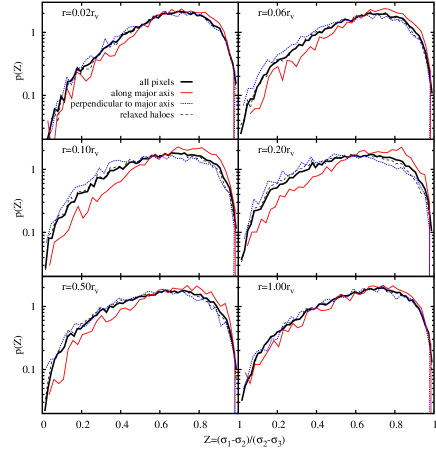
Figure 3: Triaxiality of the local velocity ellipsoids in DM haloes. The profiles show the distributions of the triaxiality parameter defined by the eq. (4). Velocity ellipsoids are predominantly prolate at all radii. The six panels show the distributions in $6$ spherical shells of radii as indicated in the left upper corners. The black (thick solid), red (solid) and blue (dotted) lines show the profiles for different pixel selection: all $48$ pixels, $8$ pixels along the halo major axis and $8$ pixels in the plane perpendicular to the major axis, respectively. The black dashed profiles are the distributions inside relaxed haloes.

4.2 Alignment

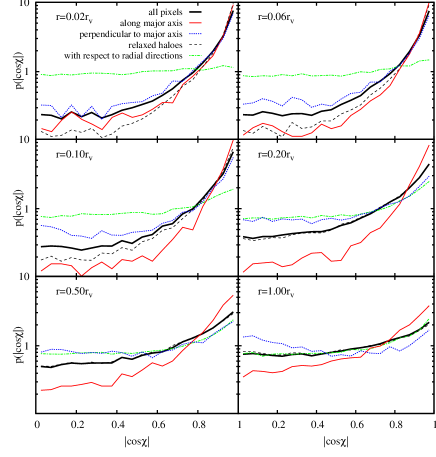
Figure 4: Alignment of the local velocity ellipsoids in DM haloes. The profiles show the distributions of cosines of the angle ($|\cos\chi|$) between the major axis of the local velocity ellipsoid and the halo major axis (except of the green dash–dotted profiles for which the angle is formed between the major axis of the local velocity ellipsoids and the local radial direction). The distributions show that the ellipsoids are preferentially parallel to the halo major axis. Degree of the alignment increases towards the halo centres. The six panels show the distribution in $6$ spherical shells of radii as indicated in the left upper corners. The black (thick solid), red (solid) and blue (dotted) lines show the profiles for different pixel selection: all $48$ pixels, $8$ pixels along the major axis and $8$ pixels in the plane perpendicular to the major axis, respectively. The black dashed profiles show the distributions inside relaxed haloes.

Figure 4 shows the distribution of the angle formed between the major axis of the local velocity ellipsoid and the halo major axis (black thick profile) or the local radial direction (green dash–dotted profile). It is clearly seen that the local velocity ellipsoids in the innermost shells display a strong alignment with the halo major axis: the black distribution is peaked at $1$, whereas the green one is flat. The alignment is the most prominent in the inner part of the haloes, at $r<0.2r_{\rm v}$, and gradually vanishes when approaching the virial sphere. In the three innermost shells (from $0.02r_{\rm v}$ to $0.10r_{\rm v}$), the median angle between the velocity ellipsoids and the halo major axis are $23$, $23$ and $25$ degrees.

The alignment of the velocity ellipsoids with the halo major axis appears to be stronger along the major axis than in the perpendicular plane (see the red solid and blue dotted profiles in Figure 4). The difference in degree of alignment between these two regions increases with radius. In both regions, however, the local velocity ellipsoids clearly tend to be aligned with the halo major axis. Exceptional deviation occurs around the virial sphere, where the distribution in the plane perpendicular to the halo major axis reveals two maxima associated with the alignment with the local radial directions and the halo major axis (see the bottom right panel of Figure 4).

The black dashed profiles in Figure 4 show the distributions in relaxed haloes. Compared to the sample of all haloes, one can see that the alignment of the local velocity velocity ellipsoids with the halo major axis is stronger in the inner parts of the relaxed haloes. On the other hand, orientations of the velocity ellipsoids at the virial sphere appear to be distributed in the same way.

In terms of the alignment of the local velocity ellipsoids, DM haloes reveal two distinct zones: the inner part ($r\mathrel{\hbox{\hbox to0.0pt{\hbox{\lower 4.0pt\hbox{$\sim$}}\hss}\hbox{$<$}}}0.2r_{\rm v}$) where the ellipsoids are aligned with the halo major axis, and the outer part ($r\mathrel{\hbox{\hbox to0.0pt{\hbox{\lower 4.0pt\hbox{$\sim$}}\hss}\hbox{$>$}}}0.5r_{\rm v}$) where alignment with the major axis is equally probable as with the radial direction. The local velocity distribution in the former is consistent with cylindrical symmetry, whereas in the latter it cannot be attributed to any simple symmetry such as spherical or cylindrical. Interestingly, both zones coincide with two characteristic regimes of the DM density profile: shallower and steeper than $\rho\propto r^{-2}$.

4.3 Local anisotropy

Here, we consider the anisotropy of the local velocity dispersion tensor. The anisotropy is defined as the ratio of the major-to-minor velocity dispersions $\sigma_{1}/\sigma_{23}$, where $\sigma_{23}^{2}=(\sigma_{2}^{2}+\sigma_{3}^{2})/2$. This definition ignores the fact of triaxiality of the velocity ellipsoids and, therefore, provides only a partial description of the ellipsoids. Nevertheless, keeping in mind that the local velocity ellipsoids are preferentially prolate, i.e. $\sigma_{1}-\sigma_{2}>\sigma_{2}-\sigma_{3}$, we expect that the $\sigma_{1}/{\sigma}_{23}$ ratio provides the first order and single-parameter description of the local velocity distribution (we will consider both the $\sigma_{1}/\sigma_{2}$ and $\sigma_{1}/\sigma_{3}$ ratios in the following section, where we compare the local and spherically averaged properties of the velocity dispersion tensor). Contrary to the definition of the anisotropy parameter $\beta$, here we assume the cylindrical symmetry of the local velocity distribution.

Figure 5 shows the distribution of the $\sigma_{1}/\sigma_{23}$ ratio in $6$ spherical shells. The distributions inside the innermost shells of radii $r\mathrel{\hbox{\hbox to0.0pt{\hbox{\lower 4.0pt\hbox{$\sim$}}\hss}\hbox{$<$}}}0.2r_{\rm v}$ depends barely on radius. The mode is equal to $1.25$ in the four innermost shells. The distributions have long tails extending to high-value anisotropies. Similar to the case of the velocity dispersion, the unrelaxed haloes appear to populate preferentially the tails of the distributions (compare the black thick and dashed profiles corresponding to the all and relaxed haloes). The anisotropy along the major axis of the virial sphere tends to be smaller than in the perpendicular plane.

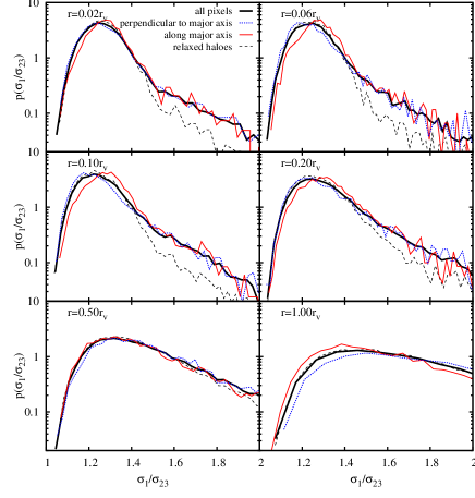
Figure 5: Anisotropy $\sigma_{1}/\sigma_{23}$ of the local velocity ellipsoids in DM haloes, where $\sigma_{23}^{2}=(\sigma_{2}^{2}+\sigma_{3}^{2})/2$. The six panels show the distributions in $6$ spherical shells of radii as indicated in the left upper corners. The colour coding is the same as in Figure 4. The local velocity ellipsoids are highly anisotropic at all radii. Typical value of the anisotropy is $\sigma_{1}/\sigma_{23}\approx 1.3$ at radii $r<0.5r_{\rm v}$ and increases to $\sigma_{1}/\sigma_{23}\approx 1.45$ at the virial radius.

The local velocity ellipsoids at the virial sphere tend to be substantially more anisotropic than in the inner parts. The mode occurs at $\sigma_{1}/\sigma_{23}=1.45$ and the distribution has a slowly decreasing tail at high values. Distributions for relaxed and unrelaxed haloes appear to be undistinguishable. The anisotropy around the halo major axis in these shells tend to be smaller than in the perpendicular plane, in contrast with the innermost shells (compare the red solid and blue dotted profiles). In Appendix, we provide an analytic model of the velocity anisotropy which recovers the measured profiles shown in Figure 5 with $~{}10$ per cent accuracy.

Similar to the alignment of the velocity ellipsoids, statistical properties of the $\sigma_{1}/\sigma_{23}$ ratio seem to differentiate the central parts of the haloes from those around the virial sphere. The former are characterised by self-similar distributions with the maximum at approximately $1.25$, whereas the latter by the distribution gradually getting wider and shifted to higher values when approaching the virial sphere. The transition between these two zones is continuous. The approximated radius of the transition is $0.2r_{\rm v}$ at which the shape of the distribution starts to deviate from that found in the shells of small radii (see the middle right panel of Figure 5).

5 Spherically averaged anisotropy

In this section, we address the problem of how to measure the anisotropy of the velocity dispersion tensor in spherical shells. It is naturally expected that the velocity dispersion computed in a shell should represent information contained in the distribution of the local properties measured in different subvolumes of the shell. In particular, spherically averaged profiles (computed in spherical shells) are expected to recover the most probable values of the local counterparts. In order to achieve this, the velocity dispersion tensor should conform with with the symmetry preferred by the local velocity ellipsoids. Strong alignment of the velocity ellipsoids with the halo major axis implies that the velocity dispersion tensor should be calculated using Cartesian coordinates of velocity vectors, as given by the eq. (3).

We used 70 spherical shells with radii equally distributed in logarithmic scale between $0.005r_{\rm v}$ and $r_{\rm v}$. Figures 6-8 show the resulting radial profiles of the anisotropy and the orientation of the velocity ellipsoids. The profiles show the median and the 50 per cent scatter of the values in the halo population. The spherically averaged profiles are compared with the local values measured in the shells defined in the previous section (points with the error bars showing the median and the $50$ per cent scatter).

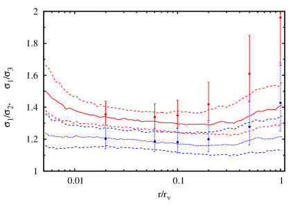
Figure 6: Radial profiles of the anisotropy of the velocity dispersion tensor calculated in spherical shells. The red solid and blue dotted lines are the profiles for $\sigma_{1}/\sigma_{2}$ and $\sigma_{1}/\sigma_{3}$, respectively (with dashed lines showing the first and third quartiles). The points with error bars represent the distributions of the local values measured in $7$ spherical shells (the median and the error bar corresponding to the $50$ per cent probability range). The $\sigma_{1}/\sigma_{2}$ and $\sigma_{1}/\sigma_{3}$ ratios computed in spherical shells reproduce the local values. Discrepancy at radii $r>0.5_{\rm v}$ occurs due to more random orientations of the velocity ellipsoids in this part of the haloes.

Figure 6 shows the profiles of the major-to-median ($\sigma_{1}/\sigma_{2}$) and the major-to-minor ($\sigma_{1}/\sigma_{3}$) velocity dispersions. The spherically averaged profiles of the anisotropy are fairly consistent with the local values at radii $r<0.5r_{\rm v}$. In this range of radii, the anisotropy is well-approximated by a flat profile with $\sigma_{1}/\sigma_{2}\approx 1.25$ and $\sigma_{1}/\sigma_{3}\approx 1.42$.

The spherically averaged anisotropy appears to underestimate the true local values at radii $r>0.5r_{\rm v}$. This is particularly well visible for the $\sigma_{1}/\sigma_{3}$ ratio, for which deviation between the median of the local and spherically averaged values of the anisotropy is of the order of $2\sigma$ at $r\approx r_{\rm v}$. This discrepancy is mostly caused by a tension between the assumed symmetry of the velocity ellipsoids and the true orientations of the local velocity ellipsoids. Larger scatter in the alignment of the local velocity dispersions (more random orientations) produces artificially more isotropic velocity dispersion tensor calculated in spherical shells.

Figure 7 shows the profiles of the angle between the major axis of the velocity ellipsoid measured in spherical shells and the halo major axis. The lines indicate the $50$ and $68$ per cent probability range of the angle measured at every radius (with the most probable values at all radii equal to $|\cos\chi|=1$). This clearly shows that the velocity ellipsoids computed in spherical shells are aligned with the halo major axis. The scatter of the angles is comparable to the scatter of the local values (compare with Figure 4).

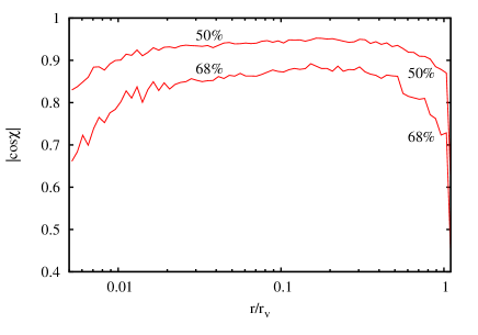
Figure 7: Alignment of the velocity ellipsoid calculated in spherical shells. The lines show the $50$ (upper) and $68$ (lower) per cent probability of the angle ($\cos\chi$) between the major axis of the velocity ellipsoid measured in spherical shells and the halo major axis. The velocity ellipsoids representing the velocity dispersion tensor calculated in spherical shells are aligned with the halo major axis.

For the sake of illustration how $\beta$ parameter misrepresents the true picture of velocity anisotropy in DM haloes, we compare in Figure 8 the spherically averaged profiles of $\beta$ and its analogue measured in a Cartesian coordinates system aligned with the semi-principle axes of the halo shape (cylindrical symmetry), i.e. $1-(\sigma_{2}^{2}+\sigma_{3}^{2})/(2\sigma_{1}^{2})$. As expected, the $\beta$ profile differs substantially from its counterpart calculated in cylindrical symmetry. In particular, nearly isotropic velocity distribution (in spherical coordinate system) in the halo centre, i.e. $\beta\approx 0$, is an effect of angular averaging over velocity ellipsoids which are strongly aligned with the halo major axis. The true orientations of the local velocity ellipsoids violate some crucial assumptions underlying the definition of the anisotropy parameter $\beta$ (radial orientations of the local velocity ellipsoids). Violation of these assumptions leads to artificially more isotropic velocity dispersion tensor (in terms of $\beta$).

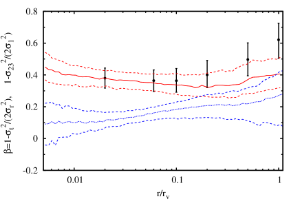
Figure 8: Radial profile of the anisotropy of the velocity dispersion tensor calculated in spherical shells. The blue dotted and red solid profiles show the anisotropy parameter $\beta=1-(\sigma_{\theta}^{2}+\sigma_{\phi}^{2})/(2\sigma_{r}^{2})$ and its counterpart defined in cylindrical symmetry, i.e. $1-(\sigma_{2}^{2}+\sigma_{3}^{3})/(2\sigma_{1}^{2})$. Black points with error bars represent the distributions of the local values measured in $7$ spherical shells (the median and the error corresponding to the $50$ per cent probability range). The anisotropy defined in cylindrical symmetry and computed in spherical shells recovers the local values. Small discrepancy at radii $r>0.5_{\rm v}$ is due to more random orientations of the velocity ellipsoids in this part of the haloes. The anisotropy parameter $\beta$ is inconsistent with the true anisotropies of the local velocity ellipsoids. Its significantly smaller values result from averaging axially symmetric velocity ellipsoids in spherical coordinate system. Dashed lines show the first and third quartiles.

In Figure 8, we also compare the spherically averaged profiles with the local values. The anisotropy defined in cylindrical symmetry recovers the local values at $r<0.5r_{\rm v}$. As in the case of Figure 6, the discrepancy at large radii is due to more random orientations of the local velocity ellipsoids. On the other hand, the anisotropy parameter $\beta$ gives erroneous impression of significantly more isotropic velocity distribution. The median $\beta$ profile lies $(2-4)\sigma$ lower than the median profile of the true local anisotropy. Using $\beta$ parameter leads to artificial isotropisation of the velocity distribution not only in the centres of DM haloes, but also at radii comparable to the virial radius.

The anisotropy parameter $\beta$ leads to a misleading picture of the true anisotropy of the velocity dispersion tensor not only when applying to spherical shells, but also locally. For example, the median $\beta$ in the equatorial pixels of the innermost shells (see Figure 1) point to nearly isotropic or weakly tangentially-biased velocity dispersion tensor, i.e. $\beta\mathrel{\hbox{\hbox to0.0pt{\hbox{\lower 4.0pt\hbox{$\sim$}}\hss}\hbox{$<$}}}0$. In fact, this is a consequence of a peculiar orientation of the local velocity ellipsoids whose major axes are preferentially parallel to the direction of the polar angle in the equatorial stripe. Averaging over the angles, a commonly used routine based on adopting the mean $(\sigma_{\theta}^{2}+\sigma_{\phi}^{2})/2$ as the variance of the tangential velocity, mixes the major and minor axes of the velocity ellipsoids and thus gives rise to an artificial isotropisation.

6 Discussion and conclusions

We studied the properties of the local velocity dispersion tensors in cluster-size simulated DM haloes. We found that the velocity ellipsoids representing the tensors are strongly aligned with the halo major axis defined as the axis minimising the moment of inertia calculated inside the virial sphere. Statistical properties of the orientations and anisotropies of the local velocity dispersion tensor do not vary with radius in the central parts of the haloes ($r<0.2r_{\rm v}$). At large radii, the orientations become gradually randomised and the ellipsoids more elongated. These two distinct zone of the haloes coincide with two characteristic regimes of the DM density profile: shallower and steeper than $\rho\propto r^{-2}$.

Alignment of the local velocity ellipsoids is inconsistent with spherically symmetric velocity distribution (radially oriented ellipsoids) that is an assumption underlying definition of the anisotropy parameter $\beta$. As a consequence, using the anisotropy parameter $\beta$ (assuming radial orientations of the local velocity ellipsoids) leads to an erroneous picture of significantly more isotropic velocity distributions than they really are. Typical ratio of the major-to-minor axis of the local velocity ellipsoids is equal to $1.3$ at radii $r<0.5r_{\rm v}$ and increases strongly with radius in the outer part of the haloes. In the light of the results presented in this paper, the assumption of spherically symmetric velocity distributions in DM haloes acts as an artificial phase mixing which may lead to a picture, in which DM haloes appear to be more equilibrated than they are. This phase mixing is one of the factors underlying the linear relation between $\beta$ and the logarithmic density slope found in simulated DM haloes (Hansen & Moore, 2006).

Similar trends of the $\beta$ profiles with the angle from the halo major axis were found in controlled simulations of halo mergers (Sparre & Hansen, 2012). This resemblance suggests that cylindrical symmetry of the velocity distributions in cosmological haloes is a remnant of major mergers.

In order to capture physical properties of the velocity anisotropy in DM haloes, we recommend to use a parameter based on the ratio of the velocity dispersions along and perpendicular to the halo major axis. A natural analogue of the classical $\beta$ parameter is

$$\beta_{\rm cyl}=1-\frac{\sigma_{2}^{2}+\sigma_{3}^{2}}{2\sigma_{1}^{2}},$$ (5)

where $\sigma_{1}$, $\sigma_{2}$ and $\sigma_{3}$ are the velocity dispersions along the major, medium, and minor axis of the halo shape ellipsoid. This parameter describes the velocity anisotropy in cylindrical symmetry with respect to the halo major axis that is consistent with the orientations of the local velocity ellipsoids. An analytic model of the velocity anisotropy is provided in Appendix.

6.1 Dynamical modelling of quasi-spherical systems

Although our studies are based on the specific sample of DM haloes (cluster–size haloes), the overall picture of the velocity ellipsoids aligned with the halo major axis may likely be generic. The argument supporting this expectation is twofold. First, the alignment is more prominent in relaxed haloes rather than in recent mergers. Second, all processes of anisotropic halo formation are common to all DM haloes and, therefore, the same mechanisms breaking spherical symmetry of the velocity distribution should operate at all scales.

Our results may have some consequences for the mass modelling of kinematical data in such objects as galaxy clusters, elliptical galaxies and dwarf spheroidals. Most of dynamical models assume spherically symmetric velocity distributions whose anisotropy is quantified with the $\beta$ parameter. It has barely ever been verified whether this assumption conforms with the true orbital structure inside these objects. This problem was addressed by Cappellari et al. (2007) in a detailed study of the stellar kinematics in massive ellipticals. It was shown that the velocity ellipsoids are preferentially aligned with the galaxy shape, on the contrary to what is assumed when considering $\beta$ parameter. Some signatures of similar orientation of the velocity ellipsoids in galaxy clusters were also demonstrated by Skielboe et al. (2012).

Alignment of the local velocity ellipsoids with the major axis may inevitably affect the mass inference with the use of dynamical models assuming radial orientations of the ellipsoids. An additional analysis is required to address this question in a fully quantitative way. However, in order to introduce the scale of the problem, we note that, in the light our results, the projected velocity dispersions in two perpendicular directions may differ by as much as $50$ per cent (see Figure 6). Using the $M_{\rm v}\propto\sigma^{3}$ scaling relation, this leads to the ratio of the mass estimates in both projections equal to $3.4$.

6.2 Observational constraints on $\beta$

The anisotropy parameter $\beta$ has been measured for a number of astrophysical systems. The estimates obtained from the stacked kinematical data of galaxies in clusters (Biviano & Katgert, 2004; Wojtak & Łokas, 2010) and the satellite galaxies around isolated hosts (Wojtak & Mamon, 2012) are fairly compatible with the spherically averaged $\beta$ profiles from the simulations. We emphasise, however, that this consistency does not imply the fact that $\beta$ describes the true orbital anisotropy, because stacking kinematical data introduces artificial sphericalisation of the phase-space distribution that is equivalent to measuring $\beta$ in spherical shells of simulated objects.

Observational constraints on the spherical anisotropy $\beta$ in individual clusters exhibit a huge variety of profiles (Benatov et al., 2006; Hwang & Lee, 2008; Wojtak & Łokas, 2010; Wojtak et al., 2009). Some measurements are far outside the margins allowed by the spherically averaged profiles of simulated clusters (see e.g. Hwang & Lee, 2008). We suspect that this substantial scatter of observational constraints on $\beta$ in individual clusters may result from ignoring the angle between the line of sight and the major axis of the velocity ellipsoids. This projection effect needs to be addressed in future in a quantitive analysis of mock kinematical data generated from cosmological simulations.

Appendix A Analytic model of the velocity anisotropy

The following simplified model captures the main features of the velocity anisotropy studied in this work. In the reference frame whose axes are aligned along the principle axes of the density distribution (with $x$, $y$ and $z$ axes corresponding to the major, medium and minor axis, respectively), the number-density $n$ as the function of velocities $\vec{V}=\{v_{x},v_{y},v_{z}\}$ and coordinates $\vec{r}=\{x,y,z\}$ can be written as :

$$n(\vec{V},\vec{r}) = \frac{n_{0}(\vec{r})}{(8\pi^{3}\sigma^{2}_{x}\sigma^{2}_{y}\sigma^{2}_{z})^{1/2}}\times$$ (6)

$$\exp\left[-\frac{v_{x}^{2}}{2\sigma^{2}_{x}}-\frac{v_{y}^{2}}{2\sigma^{2}_{y}}-\frac{v_{z}^{2}}{2\sigma^{2}_{z}}\right],$$

$$\beta_{y}(x,y,z) \equiv 1-\frac{\sigma_{y}^{2}}{\sigma^{2}_{x}}=\beta_{0y}\left(1-\frac{w_{y}^{2}(0.4+w)}{1+w}\right),$$ (7)

$$\beta_{z}(x,y,z) \equiv 1-\frac{\sigma_{z}^{2}}{\sigma^{2}_{x}}=\beta_{0z}\left(1-\frac{w_{z}^{2}(0.4+w)}{{1+w}}\right),$$ (8)

$$w_{y} = \left(\frac{y}{r_{sy}w}\right),\quad w_{z}=\left(\frac{z}{r_{sz}w}\right),$$ (9)

$$w^{2} = \left(\frac{x}{r_{sx}}\right)^{2}+\left(\frac{y}{r_{sy}}\right)^{2}+\left(\frac{z}{r_{sz}}\right)^{2},$$ (10)

where $n_{0}(x,y,z)$ is the density profile of the halo and $r_{sx}$,$r_{sy}$ and $r_{sz}$ are the scale radii of the NFW density profile (Navarro et al., 1997) fitted along the major, medium and minor axis, respectively. For cluster–size haloes studied in the paper

$$\beta_{0y}\approx 0.35,\quad\beta_{0z}\approx 0.45$$ (11)

The model assumes a Gaussian distribution of velocities with the local velocity dispersion tensor aligned with the semi-principle axes of the halo. The ratios of the medium-to-major and minor-to-major velocity dispersions are functions of the position, $\beta_{y}(x,y,z)$ and $\beta_{z}(x,y,z)$ respectively. The velocity dispersion along a given semi-principle axis of the halo is a free function of the model which may be determined using the Jeans equation. The model recovers the measurements of the velocity anisotropy shown in Figures 5,6 and 8 with $~{}10$ per cent accuracy.

References

- Allgood et al. (2006) Allgood B., Flores R. A., Primack J. R., Kravtsov A. V., Wechsler R. H., Faltenbacher A., Bullock J. S., 2006, MNRAS, 367, 1781
- Ascasibar & Gottlöber (2008) Ascasibar Y., Gottlöber S., 2008, MNRAS, 386, 2022
- Bailin & Steinmetz (2005) Bailin J., Steinmetz M., 2005, ApJ, 627, 647
- Benatov et al. (2006) Benatov L., Rines K., Natarajan P., Kravtsov A., Nagai D., 2006, MNRAS, 370, 427
- Binney (1985) Binney J., 1985, MNRAS, 212, 767
- Binney & Tremaine (2008) Binney J., Tremaine S., 2008, Galactic Dynamics: Second Edition. Princeton University Press
- Biviano & Girardi (2003) Biviano A., Girardi M., 2003, ApJ, 585, 205
- Biviano & Katgert (2004) Biviano A., Katgert P., 2004, A&A, 424, 779
- Cappellari et al. (2007) Cappellari M. et al., 2007, MNRAS, 379, 418
- Dehnen & McLaughlin (2005) Dehnen W., McLaughlin D. E., 2005, MNRAS, 363, 1057
- Dekel et al. (2005) Dekel A., Stoehr F., Mamon G. A., Cox T. J., Novak G. S., Primack J. R., 2005, Nature, 437, 707
- Diaferio (1999) Diaferio A., 1999, MNRAS, 309, 610
- Diemand et al. (2004) Diemand J., Moore B., Stadel J., 2004, MNRAS, 352, 535
- Górski et al. (2005) Górski K. M., Hivon E., Banday A. J., Wandelt B. D., Hansen F. K., Reinecke M., Bartelmann M., 2005, ApJ, 622, 759
- Hansen et al. (2010) Hansen S. H., Juncher D., Sparre M., 2010, ApJ, 718, L68
- Hansen & Moore (2006) Hansen S. H., Moore B., 2006, New Ast, 11, 333
- Hwang & Lee (2008) Hwang H. S., Lee M. G., 2008, ApJ, 676, 218
- Iannuzzi & Dolag (2012) Iannuzzi F., Dolag K., 2012, MNRAS, 427, 1024
- Jing & Suto (2002) Jing Y. P., Suto Y., 2002, ApJ, 574, 538
- Kafle et al. (2012) Kafle P. R., Sharma S., Lewis G. F., Bland-Hawthorn J., 2012, ApJ, 761, 98
- Kasun & Evrard (2005) Kasun S. F., Evrard A. E., 2005, ApJ, 629, 781
- Klypin & Holtzman (1997) Klypin A., Holtzman J., 1997, ArXiv Astrophysics e-prints
- Klypin et al. (2011) Klypin A. A., Trujillo-Gomez S., Primack J., 2011, ApJ, 740, 102
- Komatsu et al. (2009) Komatsu E. et al., 2009, ApJS, 180, 330
- Lemze et al. (2012) Lemze D. et al., 2012, ApJ, 752, 141
- Łokas (2002) Łokas E. L., 2002, MNRAS, 333, 697
- Łokas (2009) Łokas E. L., 2009, MNRAS, 394, L102
- Łokas & Mamon (2003) Łokas E. L., Mamon G. A., 2003, MNRAS, 343, 401
- Ludlow et al. (2011) Ludlow A. D., Navarro J. F., White S. D. M., Boylan-Kolchin M., Springel V., Jenkins A., Frenk C. S., 2011, MNRAS, 415, 3895
- Mamon et al. (2012) Mamon G. A., Biviano A., Boué G., 2012, ArXiv e-prints
- Merritt (1987) Merritt D., 1987, ApJ, 313, 121
- Napolitano et al. (2011) Napolitano N. R. et al., 2011, MNRAS, 411, 2035
- Navarro et al. (1997) Navarro J. F., Frenk C. S., White S. D. M., 1997, ApJ, 490, 493
- Neto et al. (2007) Neto A. F. et al., 2007, MNRAS, 381, 1450
- Newman et al. (2012) Newman A. B., Treu T., Ellis R. S., Sand D. J., Nipoti C., Richard J., Jullo E., 2012, ArXiv e-prints
- Riebe et al. (2011) Riebe K. et al., 2011, ArXiv e-prints
- Rozo et al. (2010) Rozo E. et al., 2010, ApJ, 708, 645
- Saro et al. (2012) Saro A., Bazin G., Mohr J., Dolag K., 2012, ArXiv e-prints
- Skielboe et al. (2012) Skielboe A., Wojtak R., Pedersen K., Rozo E., Rykoff E. S., 2012, ApJ, 758, L16
- Sparre & Hansen (2012) Sparre M., Hansen S. H., 2012, JCAP, 7, 42
- Walker et al. (2006) Walker M. G., Mateo M., Olszewski E. W., Bernstein R., Wang X., Woodroofe M., 2006, AJ, 131, 2114
- Walker et al. (2009) Walker M. G., Mateo M., Olszewski E. W., Peñarrubia J., Wyn Evans N., Gilmore G., 2009, ApJ, 704, 1274
- Wojtak & Łokas (2010) Wojtak R., Łokas E. L., 2010, MNRAS, 408, 2442
- Wojtak et al. (2005) Wojtak R., Łokas E. L., Gottlöber S., Mamon G. A., 2005, MNRAS, 361, L1
- Wojtak et al. (2009) Wojtak R., Łokas E. L., Mamon G. A., Gottlöber S., 2009, MNRAS, 399, 812
- Wojtak & Mamon (2012) Wojtak R., Mamon G. A., 2012, ArXiv e-prints
- Wolf et al. (2010) Wolf J., Martinez G. D., Bullock J. S., Kaplinghat M., Geha M., Muñoz R. R., Simon J. D., Avedo F. F., 2010, MNRAS, 406, 1220
- Zait et al. (2008) Zait A., Hoffman Y., Shlosman I., 2008, ApJ, 682, 835
- Zemp et al. (2009) Zemp M., Diemand J., Kuhlen M., Madau P., Moore B., Potter D., Stadel J., Widrow L., 2009, MNRAS, 394, 641
- Zemp et al. (2011) Zemp M., Gnedin O. Y., Gnedin N. Y., Kravtsov A. V., 2011, ApJS, 197, 30