Robust error estimates in weak norms for advection dominated transport problems with rough data

Abstract

We consider transient convection–diffusion equations with a velocity vector field with multiscale character and rough data. We assume that the velocity field has two scales, a coarse scale with slow spatial variation, which is responsible for advective transport and a fine scale with small amplitude that contributes to the mixing. For this problem we consider the estimation of filtered error quantities for solutions computed using a finite element method with symmetric stabilization. A posteriori error estimates and a priori error estimates are derived using the multiscale decomposition of the advective velocity to improve stability. All estimates are independent both of the Péclet number and of the regularity of the exact solution.

(xxxxxxxxxx)

AMS Subject Classification: 65M12, 65M60, 65M20, 65M15

1 Introduction

In spite of much progress in recent years the problem of deriving a posteriori error estimates and a priori error estimates for transient convection–diffusion equations is not fully understood. The difficulty is related to the wide range of different problems covered by the equation class. Indeed depending on the characteristics of the velocity field and the molecular diffusion the solutions may feature very different behaviour. From a computational point of view the complexity will depend mainly on the smoothness of data and on the Péclet number

$$\mathrm{Pe}_{L}:=\frac{UL}{\mu},$$

where $U$ is a characteristic velocity, $L$ is a lengthscale and $\mu$ the molecular diffusion. If the variations of the transport velocity are small and the data are smooth, the solution will be smooth, with moderate Sobolev norm (at least the $H^{1}$-norm) independent of the viscosity. Then a standard Galerkin method for low Péclet number flows and a stabilized finite element method for high Péclet number flows will yield accurate results. Most difficult is the case of a high Péclet number and a strongly varying, or even turbulent, velocity field, transporting a concentration that is strongly fragmented and may dilute or concentrate. In this case a computation can experience strong amplification of errors due to repeated bifurcation of streamlines and inexact representation of internal layers caused by spurious oscillations or numerical diffusion. Sometimes this regime is referred to as scalar turbulence and LES-models have been derived for the modelization of the passive scalar using filtering[17]. Such models encounter a similar Reynolds stress conundrum as the filtering of the full Navier-Stokes’ equations, and hence the modeling error is difficult to quantify. Another approach that has been attempted for this problem is heterogeneous multiscale methods[13] however in that case the underlying theory is based on homogenization and depending on a periodicity hypothesis that in most applications will not hold.

In this paper our approach is to apply a stabilized finite element method to the computation of the solution of the standard physical model, instead of a coarse grained model. The accuracy of the large scales is measured by estimating the regularized, or filtered error, related to estimating the error in local averages of the solution.

The combination of these two ingredients allows us to derive error estimates with an order in $h$, for a norm that is in a certain sense in between $H^{-1}$ and $L^{2}$, but which contains the $L^{2}$-norm of a filtered error. These estimates are robust in the sense that they do not depend on any high order Sobolev norm of the exact solution and they only have exponential growth depending on the maximum gradient of the coarse scale velocity field, under a certain scale separation assumption given below. This means that the filtered quantities considered are robust under diverging fine scale characteristic trajectories. In some sense we extract the coarse scales for which we have some (provable) accuracy from the computation.

2 The transient advection–diffusion equation

The problem that we will consider takes the following form. Let $\Omega$ be an open, convex polygonal/polyhedral subset of $\mathbb{R}^{d}$, $d=2,3$ with boundary $\partial\Omega$ and associated outward pointing normal $n_{\partial\Omega}$. We will denote the computational time interval by $I:=[0,T]$ and the space-time domain by $Q:=I\times\Omega$. Assuming homogeneous Dirichlet boundary conditions $u|_{\partial\Omega}=0$ we may formally write our problem, for $t>0$ find $u\in H^{1}_{0}(\Omega)$ such that $u(x,0)=u_{0}(x)$ in $\Omega$ and

$$\partial_{t}u+{\boldsymbol{\beta}}\cdot\nabla u-\mu\Delta u=f,\quad\mbox{ in }\Omega.$$ (1)

For the problem data we consider $u_{0}\in L^{2}(\Omega)$, $f\in L^{2}(Q)$ and let the velocity field ${\boldsymbol{\beta}}\in[C_{0}(0,T;W^{1,\infty}(\Omega))]^{d}$, such that $\nabla\cdot{\boldsymbol{\beta}}=0$, ${\boldsymbol{\beta}}\cdot n_{\partial\Omega}|_{\partial\Omega}=0$, and the molecular diffusivity $\mu\in\mathbb{R}$ with $\mu>0$. The $L^{2}$-scalar product over $X$, where $X$ can be either a space domain of $\mathbb{R}^{d}$ or a space-time domain, will be denoted by $(\cdot,\cdot)_{X}$, the $L^{2}$-scalar product over subsets $X$ of $\mathbb{R}^{d-1}$ will be denoted $\left<\cdot,\cdot\right>_{X}$. In both cases the corresponding $L^{2}$-norm is denoted by $\|\cdot\|_{X}$. We will use the notation $a\lesssim b$ to denote $a\leq Cb$ with $C$ a moderate constant independent of the mesh-parameter and the physical parameters of the problem, (except those that are assumed to be unity). We will also use the notation $a\sim b$ for $a\lesssim b$ and $b\lesssim a$.

In this paper the analysis will be restricted to velocity fields with a particular multiscale character. We will assume that the problem is normalized so that $U:=\|{\boldsymbol{\beta}}\|_{L^{\infty}(Q)}=1$ and we assume that the characteristic lengthscale is given by $L:=1$, similarly we assume that $T\sim L/\|{\boldsymbol{\beta}}\|_{L^{\infty}(Q)}=1$. Instead of making the standard assumption that $\|{\boldsymbol{\beta}}\|_{W^{1,\infty}(\Omega)}$ is small, we assume that there is a decomposition of the velocity field,

$${\boldsymbol{\beta}}=\overline{\boldsymbol{\beta}}+{\boldsymbol{\beta}}^{\prime},$$

where, for all $t$, $\|\overline{\boldsymbol{\beta}}\|_{W^{1,\infty}(\Omega)}\sim 1$ and $\|{\boldsymbol{\beta}}^{\prime}\|_{L^{\infty}(\Omega)}^{2}\sim\mu$. This allows us to define a timescale for the flow relating to the coarse scale spatial variation and the fine scale amplitude,

$$(\tau_{F})^{-1}:=\sup_{t\in I}~{}(\|\overline{\boldsymbol{\beta}}(t)\|_{W^{1,\infty}(\Omega)}+\|{\boldsymbol{\beta}}^{\prime}(t)\|_{L^{\infty}(\Omega)}^{2}/\mu)\sim 1.$$ (2)

Essentially we assume that the velocity vectorfield can be decomposed in a coarse scale, responsible for transport, that is slowly varying in space and a fine scale, responsible for mixing, that has small amplitude but may have strong spatial variation. Expressed in Péclet numbers this means that the coarse scale Péclet number may be arbitrarily high, whereas the fine scale Péclet number, based on $T$, ${\boldsymbol{\beta}}^{\prime}$ and $\mu$, must be $O(1)$. A sharper value of $\tau_{F}$ given a molecular diffusion $\mu$ and a velocity field ${\boldsymbol{\beta}}$ may be obtained by solving a certain minimzation problem in the $L^{\infty}$-norm that will be detailed in the a priori analysis.

We will assume that the coarse scale velocity satisfies a pointwise non-penetration condition on the domain boundary, $\overline{\boldsymbol{\beta}}\cdot n_{\partial\Omega}=0$.

The rough initial data or source term together with the high Péclet number and the multiscale character of the velocity field may lead to complex, low regularity solutions. More precisely solutions are smooth, due to parabolic regularity, but with large Sobolev norms, rendering standard a priori error estimates based on approximation theory worthless. Indeed classical global estimates for stabilized finite element methods for time dependent convection–diffusion equations[11, 3, 7] yield the high Péclet number error estimate:

$$\sup_{t\in I}\|(u-u_{h})(t)\|_{\Omega}+\|\mu^{\frac{1}{2}}\nabla(u-u_{h})\|_{Q}\leq Ch^{\frac{3}{2}}(1+\mathrm{Pe}_{h}^{-1/2})|u|_{L^{2}(I;H^{2}(\Omega))}$$ (3)

where $u_{h}$ denotes the approximate solution using piecewise affine approximation. Even though $|u|_{H^{2}(\Omega)}$ is huge in the presence of layers, stabilized methods are relevant for this case since one may derive localized error estimates, showing that perturbations can not spread too far upwind of crosswind in the stationary case[15, 12, 5], or spread too far across characteristics in the transient case[18]. The reason this works is that $|u|_{H^{2}(\omega)}$ can be assumed to be small in a part of the domain $\omega\subset\Omega$ provided $u$ has no layers in a neighbourhood of $\omega$. In the estimates the bad part can be cut away using a suitably chosen weight function. This technique is not applicable in the present case, since the strong oscillations of the velocity field and the nonsmoothness of $u_{0}$ and $f$, makes it unrealistic to assume that $|u|_{H^{2}(\omega)}$ is small in any part of the domain. The aim of this paper is to show that also in this case, stabilized finite element methods produce an improved solution compared to that of standard Galerkin and that we can indeed derive error estimates for some large scale quantities defined by differential filtering.

Drawing from earlier ideas on a posteriori error estimation[2, 14] we propose to estimate a regularized error, or in other terms, work in a norm in between $H^{-1}$ and $L^{2}$. Indeed let the regularized error $\tilde{e}$ be defined by the partial differential equation

$$-\mathfrak{h}\Delta\tilde{e}+\tilde{e}=(u-u_{h})(\cdot,T),$$ (4)

with $\tilde{e}|_{\partial\Omega}=0$, $\mathfrak{h}\in\mathbb{R}^{+}$. We then prove that

$$\|\tilde{e}\|_{\mathfrak{h}}:=\left(\|\mathfrak{h}^{\frac{1}{2}}\nabla\tilde{e}\|^{2}_{\Omega}+\|\tilde{e}\|^{2}_{\Omega}\right)^{\frac{1}{2}}\lesssim C_{T,f,u_{0}}\left(\frac{h}{\mathfrak{h}}\right)^{\frac{1}{2}}.$$

The constant $C_{T,f,u_{0}}$ of the estimates is independent both of the Péclet number and of the regularity of the exact solution. It depends on the data of the problem and the main time dependence is a factor

$$\exp\left(c_{\Lambda}\frac{T}{\tau_{F}}\right)$$

where $T$ denotes the final time of the simulation and $c_{\Lambda}$ is a moderate constant. This factor limits the applicability of the analysis to time intervals of the size $\tau_{F}$ and hence limits the validity of the arguments to smooth vectorfields ${\boldsymbol{\beta}}$ or those satisfying the scale separation case discussed above.

The parameter $\mathfrak{h}$ can be related to a filter width $\delta$ by $\mathfrak{h}:=\delta^{2}$, or an artificial diffusivity for elliptic smoothing. In both cases we see that the hidden constant includes dimensional quantities of order unity. For $\mathfrak{h}$ constant the results can be interpreted as $H^{-1}$-norm error estimates and in this norm the convergence rate $h^{\frac{1}{2}}$ is most likely optimal.

Below we will first recall the standard $L^{2}$-norm error analysis for high Péclet number flow and see what is required of data to obtain an estimate with an order that is fully independent of $\mu$ (that is, we control suitable Sobolev norms of $u$ a priori). Then, we consider error estimation of filtered quantities and we obtain a posteriori error estimates. A priori estimates for rough solutions in the general case follow directly using standard stability estimates of the discrete solution.

The weak formulation of equation (1) reads, for $t>0$, find $u\in H^{1}_{0}(\Omega)$ such that $u(x,0)=u_{0}(x)$ and

$$(\partial_{t}u,v)_{\Omega}+a(u,v)=(f,v)_{\Omega},\quad\forall v\in H^{1}_{0}(\Omega),$$ (5)

where $a(\cdot,\cdot)$ is defined by:

$$a(u,v):=(\beta\cdot\nabla u,v)_{\Omega}+(\mu\nabla u,\nabla v)_{\Omega}.$$

3 Stability and regularity of the solution

Since the constant in the estimate (3) depends on the $H^{2}$-norm of the solution it is important to understand what quantities it is possible to control, if robustness in $\mu$ is required. In this section we will first show the standard global regularity estimate for parabolic problems detailing the dependence of the constant on $\mu$. We will then show an estimate where the constant is independent of $\mu$, but not of $\tau_{F}$. In both cases we will need to assume that data have some smoothness.

Lemma 3.1.

(Standard energy estimate) Let $u$ be the solution of (5), then there holds

$$\sup_{t\in I}\|u(t)\|_{\Omega}+\|\mu^{\frac{1}{2}}\nabla u\|_{Q}\lesssim\int_{I}\|f(t)\|_{\Omega}\mbox{d}t+\|u_{0}\|_{\Omega}.$$ (6)

Proof 3.2.

We take $v=u$ in (5) and then use that

$$\int_{I}(f,u)_{\Omega}~{}\mbox{d}t\leq\sup_{t\in I}\|u(\cdot,t)\|_{\Omega}\int_{I}\|f\|_{\Omega}~{}\mbox{d}t$$

from which the bound on $\sup_{t\in I}\|u(t)\|_{\Omega}$ follows. This bound is then used to get the $H^{1}$-bound, which is a consequence of the equation (5) and the equality

$$\|\mu^{\frac{1}{2}}\nabla u\|_{Q}^{2}=\int_{I}a(u,u)~{}\mbox{d}t.$$

Theorem 3.3.

Let $u$ be the weak solution of (1), with $f\in L^{2}(Q)$ and $u_{0}\in H^{1}_{0}(\Omega)$. Assume that $\Omega$ is a convex domain. Then there holds

$$\sup_{t\in I}\|\mu^{\frac{1}{2}}\nabla u(t)\|_{\Omega}+|\mu u|_{L^{2}(I;H^{2}(\Omega))}\lesssim\mu^{-1/2}\left(\int_{I}\|f(t)\|_{\Omega}\mbox{d}t+\|u_{0}\|_{\Omega}\right)\\ +\|f\|_{Q}+\|\mu^{\frac{1}{2}}\nabla u_{0}\|_{\Omega}.$$

Proof 3.4.

Multiplying (1) with $-\mu\Delta u$, integrating over the space time domain $Q^{*}:=(0,t^{*})\times\Omega$, with $t^{*}<T$ and applying the Cauchy-Schwarz inequality and the arithmetic-geometric inequality gives

$$\|\mu^{\frac{1}{2}}\nabla u(t^{*})\|^{2}_{\Omega}+\|\mu\Delta u\|^{2}_{Q^{*}}\leq\|{\boldsymbol{\beta}}\|^{2}_{L^{\infty}(Q^{*})}\mu^{-1}\|\mu^{\frac{1}{2}}\nabla u\|_{Q^{*}}^{2}+\frac{1}{4}\|\mu\Delta u\|^{2}_{Q^{*}}\\ +\|f\|^{2}_{Q^{*}}+\|\mu^{\frac{1}{2}}\nabla u_{0}\|^{2}_{\Omega}.$$

It follows from (6) that

$$\sup_{t\in I}\|\mu^{\frac{1}{2}}\nabla u(t)\|_{\Omega}\lesssim\|{\boldsymbol{\beta}}\|_{L^{\infty}(Q)}\mu^{-1/2}(\int_{I}\|f(t)\|_{\Omega}\mbox{d}t+\|u_{0}\|_{\Omega})+\|f\|_{Q}+\|\mu^{\frac{1}{2}}\nabla u_{0}\|_{\Omega}$$

and

$$\|\mu\Delta u\|_{Q}\lesssim\|{\boldsymbol{\beta}}\|_{L^{\infty}(Q)}\mu^{-1/2}(\int_{I}\|f(t)\|_{\Omega}\mbox{d}t+\|u_{0}\|_{\Omega})+\|f\|_{Q}+\|\mu^{\frac{1}{2}}\nabla u_{0}\|_{\Omega}.$$

We conclude using elliptic regularity, recalling that the advection velocity is normalised.

Remark 3.5.

Observe that it follows that $\|\nabla u\|_{Q}\lesssim\mu^{-1/2}$, $\sup_{t\in I}\|\nabla u\|_{\Omega}\lesssim\mu^{-1}$ and $\|u\|_{L^{2}(I;H^{2}(\Omega))}\lesssim\mu^{-3/2}$. Hence we conclude that the regularity estimates of Lemma 3.1 and Theorem 3.3 both are sensitive to the variation of the diffusivity and can only be used when $\mathrm{Pe_{h}}\leq 1$. Also some regularity of the inital data is needed, $u_{0}\in H^{1}_{0}(\Omega)$. Revisiting the estimate (3) in this context we get

$$\|\mu^{\frac{1}{2}}\nabla(u-u_{h})\|_{Q}\lesssim\Bigl{[}\left(\frac{h}{\mu}\right)^{3/2}+\left(\frac{h}{\mu}\right)\Bigr{]}(\int_{I}\|f(t)\|_{\Omega}\mbox{d}t+\|u_{0}\|_{\Omega}+\mu^{\frac{1}{2}}\|f\|_{Q}+\|\mu^{\frac{1}{2}}\nabla u_{0}\|_{\Omega}).$$ (7)

This estimate is clearly useless when $\mathrm{Pe}_{h}>1$.

We will now show that using the scale separation of the advection field and assuming some more regularity of data, all inverse powers of the diffusivity may be avoided. The price to pay is an exponential constant, which however, under our assumption on the velocity field remains moderate. It should be noted that if no assumption is made on the velocity field, sharp layers in the velocity may result in $O(\mu^{\frac{1}{2}})$ width layers in the solution $u$. The corresponding growth in the $H^{1}$-norm, makes global estimates independent of $\mu$ impossible.

Theorem 3.6.

Let $u$ be the weak solution of (1), with $\Omega$ convex, $f\in L^{2}(I;H^{1}_{0}(\Omega))$ and $u_{0}\in H^{1}_{0}(\Omega)$. Then for $0<\mathfrak{h}$, $\mu<1$, there holds

$$\sup_{t\in I}\|u(\cdot,t)\|_{\mathfrak{h}}+|(\mathfrak{h}\mu)^{\frac{1}{2}}u|_{L^{2}(I;H^{2}(\Omega))}+T^{-\frac{1}{2}}\|\mathfrak{h}^{\frac{1}{2}}\nabla u\|_{Q}+T^{-\frac{1}{2}}\|\mathfrak{h}^{\frac{1}{2}}\partial_{t}u\|_{Q}\\ \lesssim C_{T}(\mathfrak{h}^{\frac{1}{2}}\|f\|_{L^{2}(I;H^{1}(\Omega))}+\int_{I}\|f\|\mbox{d}t+\|u_{0}\|_{\mathfrak{h}}),$$ (8)

with $C_{T}=e^{\left(c_{\Lambda}\frac{T}{\tau_{F}}\right)},$ where $\tau_{F}$ is given by (2) and $c_{\Lambda}$ is a moderate constant .

Proof 3.7.

First observe that we know from Theorem 3.3 that $u\in L^{2}(I;H^{2}(\Omega))$, so the important addition in Theorem 3.6 is the control of $\|u(\cdot,t)\|_{\mathfrak{h}}$ that is robust $\mu$. Multiply equation (1) by $-\mathfrak{h}\Delta u$ and integrate over $Q^{*}:=(0,t^{*})\times\Omega$ with $t^{*}<T$, to obtain

$$\frac{1}{2}\|\mathfrak{h}^{\frac{1}{2}}\nabla u(\cdot,t^{*})\|^{2}_{\Omega}-({\boldsymbol{\beta}}\cdot\nabla u,\mathfrak{h}\Delta u)_{Q^{*}}+\|(\mu\mathfrak{h})^{\frac{1}{2}}\Delta u\|^{2}_{Q^{*}}\\ \lesssim(\nabla f,\mathfrak{h}\nabla u)_{Q^{*}}+\frac{1}{2}\|\mathfrak{h}^{\frac{1}{2}}\nabla u_{0}\|^{2}_{\Omega}.$$

The second term in the left hand side does not have a sign and requires some further consideration. First split the velocity field in the large and the fine scale component,

$$-({\boldsymbol{\beta}}\cdot\nabla u,\mathfrak{h}\Delta u)_{Q^{*}}=-(\overline{\boldsymbol{\beta}}\cdot\nabla u,\mathfrak{h}\Delta u)_{Q^{*}}-({\boldsymbol{\beta}}^{\prime}\cdot\nabla u,\mathfrak{h}\Delta u)_{Q^{*}},$$

then integrate by parts in the term representing the large scale transport, noting that if $t_{1}$ and $t_{2}$ denotes the two orthonormal tangential vectors to $\partial\Omega$,

$$\overline{\boldsymbol{\beta}}\cdot\nabla u|_{\partial\Omega}=\underbrace{\overline{\boldsymbol{\beta}}\cdot n_{\partial\Omega}}_{=0}\nabla u\cdot n_{\partial\Omega}|_{\partial\Omega}+\sum_{i=1}^{2}\overline{\boldsymbol{\beta}}\cdot t_{i}(\underbrace{\nabla u\cdot t_{i}}_{=0})|_{\partial\Omega}=0.$$

Recalling that $u\in L^{2}(I;H^{2}(\Omega))$ and $\overline{\boldsymbol{\beta}}\in C^{0}(I;W^{1,\infty}(\Omega))$ we have $\overline{\boldsymbol{\beta}}\cdot\nabla u\in L^{2}(I;H_{0}^{1}(\Omega))$. Then the following integration by parts is justified

$$-(\overline{\boldsymbol{\beta}}\cdot\nabla u,\mathfrak{h}\Delta u)_{Q^{*}}=(\nabla(\overline{\boldsymbol{\beta}}\cdot\nabla u),\mathfrak{h}\nabla u)_{Q^{*}}.$$

Note that by the product rule

$$(\nabla(\overline{\boldsymbol{\beta}}\cdot\nabla u),\mathfrak{h}\nabla u)_{Q^{*}}=\sum_{i=1}^{d}((\partial_{x_{i}}\overline{\boldsymbol{\beta}})\cdot\nabla u,\mathfrak{h}\partial_{x_{i}}u)_{Q^{*}}+\sum_{i=1}^{d}(\overline{\boldsymbol{\beta}}\cdot(\partial_{x_{i}}\nabla u),\mathfrak{h}\partial_{x_{i}}u)_{Q^{*}}.$$ (9)

For the first sum of the right hand side we have

$$\sum_{i=1}^{d}((\partial_{x_{i}}\overline{\boldsymbol{\beta}})\cdot\nabla u,\mathfrak{h}\partial_{x_{i}}u)_{Q^{*}}=((\nabla_{S}\overline{\boldsymbol{\beta}})\cdot\nabla u,\mathfrak{h}\nabla u)_{Q^{*}}$$

where $\nabla_{S}$ denotes the symmetric part of the gradient tensor. Similarly we obtain for the second part

$$\sum_{i=1}^{d}(\overline{\boldsymbol{\beta}}\cdot(\partial_{x_{i}}\nabla u),\mathfrak{h}\partial_{x_{i}}u)_{Q^{*}}=\sum_{i=1}^{d}\sum_{j=1}^{d}(\overline{\beta}_{j}(\partial_{x_{i}}\partial_{x_{j}}u),\mathfrak{h}\partial_{x_{i}}u)_{Q^{*}}\\ =\sum_{i=1}^{d}\sum_{j=1}^{d}(\overline{\beta}_{j}(\partial_{x_{j}}\partial_{x_{i}}u),\mathfrak{h}\partial_{x_{i}}u)_{Q^{*}}=\sum_{i=1}^{d}(\overline{\boldsymbol{\beta}}\cdot\nabla\partial_{x_{i}}u,\mathfrak{h}\partial_{x_{i}}u)_{Q^{*}}.$$ (10)

By the divergence theorem, recalling that $\overline{\boldsymbol{\beta}}\cdot n_{\partial\Omega}=0$, we have

$$\sum_{i=1}^{d}(\overline{\boldsymbol{\beta}}\cdot\nabla\partial_{x_{i}}u,\mathfrak{h}\partial_{x_{i}}u)_{Q^{*}}=-\frac{1}{2}\sum_{i=1}^{d}(\nabla\cdot\overline{\boldsymbol{\beta}}\,\partial_{x_{i}}u,\mathfrak{h}\partial_{x_{i}}u)_{Q^{*}}.$$

We conclude that, with $\mathcal{I}$ denoting the identity matrix,

$$-(\overline{\boldsymbol{\beta}}\cdot\nabla u,\mathfrak{h}\Delta u)_{Q^{*}}=((\nabla_{S}\overline{\boldsymbol{\beta}}-\frac{1}{2}\nabla\cdot\overline{\boldsymbol{\beta}}\mathcal{I})\nabla u,\mathfrak{h}\nabla u)_{Q^{*}}$$ (11)

Observing that

$$({\boldsymbol{\beta}}^{\prime}\cdot\nabla u,\mathfrak{h}\Delta u)_{Q^{*}}\leq\|\mathfrak{h}^{\frac{1}{2}}|{\boldsymbol{\beta}}^{\prime}|\mu^{-1/2}\nabla u\|_{Q^{*}}\|(\mathfrak{h}\mu)^{\frac{1}{2}}\Delta u\|_{Q^{*}}\\ \leq\frac{1}{2}\|\mathfrak{h}^{\frac{1}{2}}|{\boldsymbol{\beta}}^{\prime}|\mu^{-1/2}\nabla u\|^{2}_{Q^{*}}+\frac{1}{2}\|(\mathfrak{h}\mu)^{\frac{1}{2}}\Delta u\|_{Q^{*}}^{2}$$ (12)

we have,

$$\frac{1}{2}\|\mathfrak{h}^{\frac{1}{2}}\nabla u(\cdot,t^{*})\|^{2}_{\Omega}+\frac{1}{2}\|(\mu\mathfrak{h})^{\frac{1}{2}}\Delta u\|^{2}_{Q^{*}}\leq\int_{0}^{t^{*}}(\nabla f,\mathfrak{h}\nabla u)_{\Omega}\\ +\frac{1}{2}\|\mathfrak{h}^{\frac{1}{2}}\nabla u_{0}\|^{2}_{\Omega}+(\Lambda(\overline{\boldsymbol{\beta}},{\boldsymbol{\beta}}^{\prime},\mu)\nabla u,\mathfrak{h}\nabla u)_{\Omega}$$ (13)

where

$$\Lambda(\overline{\boldsymbol{\beta}},{\boldsymbol{\beta}}^{\prime},\mu):=\nabla_{S}\overline{\boldsymbol{\beta}}-\frac{1}{2}\nabla\cdot\overline{\boldsymbol{\beta}}\mathcal{I}+\frac{1}{2}|{\boldsymbol{\beta}}^{\prime}|^{2}\mu^{-1}.$$

Defining

$$\tilde{\tau}_{F}^{-1}:=\sup_{t\in I}\inf_{\begin{subarray}{c}\overline{\boldsymbol{\beta}}\in W^{1,\infty}(\Omega)\\ \overline{\boldsymbol{\beta}}\cdot n=0\mbox{ on }\partial\Omega\end{subarray}}\sigma_{p}(\Lambda(\overline{\boldsymbol{\beta}},{\boldsymbol{\beta}}^{\prime},\mu))$$ (14)

where $\sigma_{p}(A)$ denotes the largest positive eigenvalue of the matrix $A$, we may write

$$\|\mathfrak{h}^{\frac{1}{2}}\nabla u(\cdot,t^{*})\|^{2}_{\Omega}+\|(\mu\mathfrak{h})^{\frac{1}{2}}\Delta u\|^{2}_{Q^{*}}\leq t^{*}\|\mathfrak{h}^{\frac{1}{2}}\nabla f\|^{2}_{Q^{*}}\\ +((t^{*})^{-1}+2\tilde{\tau}_{F}^{-1})\|\mathfrak{h}^{\frac{1}{2}}\nabla u\|^{2}_{Q^{*}}+\|\mathfrak{h}^{\frac{1}{2}}\nabla u_{0}\|^{2}_{\Omega}.$$ (15)

The claim regarding the control of the space derivatives now follows after an application of Gronwall’s lemma, yielding

$$\|\mathfrak{h}^{\frac{1}{2}}\nabla u(\cdot,t^{*})\|^{2}_{\Omega}+\|(\mathfrak{h}\mu)^{\frac{1}{2}}\Delta u\|^{2}_{Q^{*}}\lesssim e^{2t^{*}/\tilde{\tau}_{F}}\left(\|\mathfrak{h}^{\frac{1}{2}}\nabla f\|_{Q^{*}}^{2}+\|\mathfrak{h}^{\frac{1}{2}}\nabla u_{0}\|^{2}_{\Omega}\right).$$ (16)

Combining this estimate with estimate (6) yields the claim for the first two terms in the left hand side of equation (8). Note that we also have

$$T^{-\frac{1}{2}}\|\mathfrak{h}^{\frac{1}{2}}\nabla u\|^{2}_{Q}\lesssim\sup_{t\in I}\|\mathfrak{h}^{\frac{1}{2}}\nabla u(\cdot,t)\|^{2}_{\Omega}\lesssim e^{2T/\tilde{\tau}_{F}}\left(\|\mathfrak{h}^{\frac{1}{2}}\nabla f\|_{Q}^{2}+\|\mathfrak{h}^{\frac{1}{2}}\nabla u_{0}\|^{2}_{\Omega}\right).$$ (17)

For the control of the time derivative, simply multiply the equation with $\mathfrak{h}\partial_{t}u$ and integrate to obtain

$$\frac{1}{2}\|\mathfrak{h}^{\frac{1}{2}}\partial_{t}u\|^{2}_{Q}\leq-({\boldsymbol{\beta}}\cdot\nabla u,\mathfrak{h}\partial_{t}u)_{Q}+\frac{1}{2}\|\mathfrak{h}^{\frac{1}{2}}f\|^{2}_{Q}+\frac{1}{2}\|(\mathfrak{h}\mu)^{\frac{1}{2}}\nabla u_{0}\|^{2}_{\Omega}\\ \leq\|{\boldsymbol{\beta}}\|_{L^{\infty}(Q)}\|\mathfrak{h}^{\frac{1}{2}}\nabla u\|_{Q}\|\mathfrak{h}^{\frac{1}{2}}\partial_{t}u\|_{Q}+\frac{1}{2}\|\mathfrak{h}^{\frac{1}{2}}f\|^{2}_{Q}+\frac{1}{2}\|(\mathfrak{h}\mu)^{\frac{1}{2}}\nabla u_{0}\|^{2}_{\Omega}$$

and we conclude using the estimate (17) and the observation that comparing the definitions (2) and (14) we have $\tau_{F}\sim\tilde{\tau}_{F}$, with a moderate constant. Since $\Omega$ is convex, elliptic regularity holds

$$|(\mu\mathfrak{h})^{\frac{1}{2}}u|_{L^{2}(I;H^{2}(\Omega))}\lesssim\|(\mu\mathfrak{h})^{\frac{1}{2}}\Delta u\|_{Q}.$$

The claim follows.

4 Finite element discretizations

Let $\{\mathcal{T}_{h}\}$ be a family of nonoverlapping conforming, quasi uniform triangulations, $\mathcal{T}_{h}:=\{K\}_{h}$ where the simplices $K$ have diameter $h_{K}$ and that is indexed by $h:=\max h_{K}$. We let the set of interior faces $\{F\}_{h}$ of a triangulation $\mathcal{T}_{h}$ be denoted by $\mathcal{F}$.

We will consider a standard finite element space of piecewise polynomial, continuous functions

$$V^{0}_{h}:=\{v_{h}\in H_{0}^{1}(\Omega):v_{h}|_{K}\in P_{k}(K),\quad\forall K\in\mathcal{T}_{h}\},$$

where $P_{k}(K)$ denotes the polynomials of degree less than or equal to $k$ on $K$. The following inverse inequalities are known to hold on $V^{0}_{h}$,

$$\|\nabla v_{h}\|_{K}\leq c_{i}h_{K}^{-1}\|v_{h}\|_{K}$$ (18)

and

$$\|v_{h}\|_{\partial K}\leq c_{t}h_{K}^{-1/2}\|v_{h}\|_{K}.$$ (19)

We let $\pi_{h}:L^{2}(\Omega)\rightarrow V^{0}_{h}$ denote the $L^{2}$-projection defined by $\pi_{h}v\in V^{0}_{h}$ such that $(\pi_{h}v,w_{h})_{\Omega}=(v,w_{h})_{\Omega}$ for all $w_{h}\in V^{0}_{h}$.

The standard finite element method is then obtained by restricting the weak formulation (5) to the discrete space $V_{h}^{0}$. For $t>0$ find $u_{h}\in V_{h}^{0}$ such that $u_{h}(x,0)=\pi_{h}u_{0}(x)$ and

$$(\partial_{t}u_{h},v_{h})_{\Omega}+a(u_{h},v_{h})=(f,v_{h})_{\Omega},\quad\forall v_{h}\in V_{h}^{0}.$$ (20)

Taking $v_{h}=u_{h}$ we immediately get the stability estimate

$$\sup_{t\in(0,T]}\|u_{h}(t)\|_{\Omega}+\left(\int_{0}^{T}\|\mu^{\frac{1}{2}}\nabla u_{h}\|^{2}_{\Omega}~{}\mbox{d}t\right)^{\frac{1}{2}}\lesssim\int_{0}^{T}\|f\|_{\Omega}~{}\mbox{d}t+\|u_{0}\|_{\Omega}.$$

When the Péclet number is low this approximations of the parabolic equation may be analysed using well known finite element techniques, see Thomée[19].

However when the local Péclet number is high, the problem is a singularly perturbed parabolic problem and the stability properties of the standard Galerkin method are in general insufficient for optimal convergence. In particular in the presence of layers the whole computational domain may be polluted by spurious oscillations, but as can be seen in Figure 1, convergence order is lost also for smooth solutions. In this case we study a Gaussian function convected one turn in a disc. Time discretization is performed with the Crank-Nicolson method and we compare the result of the standard Galerkin method with those obtained using symmetric stabilization methods.

In this paper we will consider symmetric stabilization methods only, however at least for time constant ${\boldsymbol{\beta}}$ one can obtain similar results for the SUPG-method.

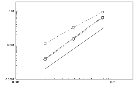
Figure 1: Convergence in the $L^{2}$-norm plotted against the timestep $\tau=h$, of the stabilized (dashed line for explicit and dotted line for implicit treatment of the stabilization operator) and unstabilized (dash-dot) Crank-Nicolson method. The full line shows optimal second order convergence.

4.1 Symmetric stabilization methods

In the last ten years there has been an important development in the field of high order symmetric stabilization methods. Such methods are typically obtained by the addition of a weakly consistent, dissipative operator to the formulation. Some of the more important symmetric stabilization methods present in the literature are the subgrid viscosity method suggested by Guermond[10], the orthogonal subscale method proposed by Codina[8], the local project method introduced by Becker and Braack[1], the discontinuous Galerkin method[16] and the continuous interior penalty (CIP) method suggested by Douglas and Dupont[9] and analysed by Burman and Hansbo[6]. The analysis that we propose herein will rely on an orthogonality argument and hence is valid only for the orthogonal subscales, the discontinuous Galerkin method and for the CIP-method. For simplicity we will focus on the latter below.

Herein we will assume that the following holds:

1. $s_{h}(\cdot,\cdot):V_{h}^{0}\times V_{h}^{0}\mapsto\mathbb{R}$ is a symmetric, bilinear and positive semi definite operator.

2. For the $L^{2}$-projection $\pi_{h}:L^{2}(\Omega)\mapsto V_{h}^{0}$ there holds

   • Approximability, $\forall u\in H^{1}_{0}(\Omega)\cap H^{k+1}(\Omega)$

     $$\|h^{-1/2}(u-\pi_{h}u)\|_{\Omega}+\|\mu^{\frac{1}{2}}\nabla(u-\pi_{h}u)\|_{\Omega}\lesssim(h^{\frac{1}{2}}+\mu^{\frac{1}{2}})h^{k}|u|_{H^{k+1}(\Omega)},$$ (21)

   • Stability and weak consistency of the stabilization operator

     $$s_{h}(u_{h},\pi_{h}v)\lesssim s_{h}(u_{h},u_{h})^{\frac{1}{2}}h^{\frac{1}{2}}\|\nabla v\|_{\Omega},\quad\forall u_{h}\in V_{h}^{0},\,v\in H^{1}(\Omega).$$ (22)

     $$s_{h}(\pi_{h}u,\pi_{h}u)\lesssim h^{k+1/2}|u|_{H^{k+1}(\Omega)},\quad\forall u\in H^{k+1}(\Omega).$$ (23)

   • Enhanced continuity of the convection term: for all $v_{h}\in V_{h}^{0}$ and ${\boldsymbol{\beta}}\in W^{1,\infty}(\Omega)$, with ${\boldsymbol{\beta}}\cdot n_{\partial\Omega}|_{\partial\Omega}=0$, there holds

     $$|(u-\pi_{h}u,{\boldsymbol{\beta}}\cdot\nabla v_{h})_{\Omega}|\lesssim\|{\boldsymbol{\beta}}\|_{W^{1,\infty}(\Omega)}\|u-\pi_{h}u\|_{\Omega}\|v_{h}\|_{\Omega}\\ +\|{\boldsymbol{\beta}}\|^{\frac{1}{2}}_{L^{\infty}(\Omega)}\|h^{-1/2}(u-\pi_{h}u)\|_{\Omega}s_{h}(v_{h},v_{h}).$$ (24)

As an example consider the CIP-method. Here $s_{h}(\cdot,\cdot)$ consists in a penalty on the jump of the gradient over element faces, and takes the form

$$s_{h}(u_{h},v_{h}):=\gamma\sum_{F\in\mathcal{F}}\left<h^{2}_{F}\|{\boldsymbol{\beta}}\cdot n_{F}\|_{L^{\infty}(F)}[\![\nabla u_{h}\cdot n_{F}]\!],[\![\nabla v_{h}\cdot n_{F}]\!]\right>_{F}$$

where $F$ denotes the faces in the mesh, $[\![x]\!]$ the jump of $x$ over $F$, the orientation is not important, $n_{F}$ a fixed but arbitrary normal associated to each face. In the analysis below we will for simplicity use this stabilization operator.

The stabilized finite element method then takes the form, for $t>0$ find $u_{h}\in V_{h}^{0}$ such that $u_{h}(x,0)=\pi_{h}u_{0}(x)$ and

$$(\partial_{t}u_{h},v_{h})_{\Omega}+a(u_{h},v_{h})+s_{h}(u_{h},v_{h})=(f,v_{h})_{\Omega},\quad\forall v_{h}\in V_{h}^{0}.$$ (25)

For the satisfaction of the assumptions (21)–(24) we refer to Ref. BFH06. Although in that reference Nitsche-type boundary conditions are used, the same argument may be shown to work whenever ${\boldsymbol{\beta}}\cdot\nabla v_{h}|_{\partial\Omega}=0$, which is the case herein. For completeness we show how to obtain (24) in our case. We also show that the flow field ${\boldsymbol{\beta}}$ in the stabilization operator may be replaced by $\overline{\boldsymbol{\beta}}$ at the cost of a nonessential perturbation. The key result is the following Lemma.

Lemma 4.1.

Assume that for $k\geq 2$ no element in $\mathcal{T}_{h}$ has more than one face intersecting $\partial\Omega$. Then there holds for all $u_{h}\in V_{h}^{0}$,

$$\inf_{v_{h}\in V_{h}^{0}}\|h^{\frac{1}{2}}(\pi_{0}{\boldsymbol{\beta}}\cdot\nabla u_{h}-v_{h})\|_{\Omega}\lesssim s_{h}(u_{h},u_{h})^{\frac{1}{2}}+h^{\frac{1}{2}}\|{\boldsymbol{\beta}}\|_{W^{1,\infty}(\Omega)}\|u_{h}\|_{\Omega},$$

where $\pi_{0}{\boldsymbol{\beta}}$ is a piecewise constant approximation of ${\boldsymbol{\beta}}$ that will be defined below.

Proof 4.2.

Let $\pi_{0}{\boldsymbol{\beta}}$ be the projection onto element wise constants such that for every $K$ that has no face on the boundary there holds

$$\int_{K}\pi_{0}{\boldsymbol{\beta}}~{}\mbox{d}x=\int_{K}{\boldsymbol{\beta}}~{}\mbox{d}x.$$

On elements adjacent to the boundary define $\pi_{0}{\boldsymbol{\beta}}$ by

$$\int_{\partial K\cap\partial\Omega}\pi_{0}{\boldsymbol{\beta}}\cdot n_{\partial\Omega}~{}\mbox{d}x=\int_{\partial K\cap\partial\Omega}{\boldsymbol{\beta}}\cdot n_{\partial\Omega}~{}\mbox{d}x$$

and

$$\int_{\partial K\cap\partial\Omega}\pi_{0}{\boldsymbol{\beta}}\cdot t_{i}~{}\mbox{d}x=\int_{\partial K\cap\partial\Omega}{\boldsymbol{\beta}}\cdot t_{i}~{}\mbox{d}x,\quad i=1,...,d-1.$$

It follows from standard approximation that for all $K\in\mathcal{T}_{h}$,

$$\|{\boldsymbol{\beta}}-\pi_{0}{\boldsymbol{\beta}}\|_{L^{\infty}(K)}\lesssim\|{\boldsymbol{\beta}}\|_{W^{1,\infty}(K)}h_{K}.$$

Note that for any element $K$ with one face on the boundary there holds

$$\pi_{0}{\boldsymbol{\beta}}\cdot\nabla u_{h}|_{\partial\Omega\cap\partial K}=\underbrace{\pi_{0}{\boldsymbol{\beta}}\cdot n_{\partial\Omega}}_{=0}\nabla u_{h}\cdot n_{\partial\Omega}|_{\partial\Omega\cap\partial K}+\sum_{i=1}^{d}\pi_{0}{\boldsymbol{\beta}}\cdot t_{i}(\underbrace{\nabla u_{h}\cdot t_{i}}_{=0})|_{\partial\Omega\cap\partial K}=0.$$

For $k=1$, if an element $K$ has two faces on the boundary, then $u_{h}\equiv 0$ in that element and therefore $\pi_{0}{\boldsymbol{\beta}}\cdot\nabla u_{h}|_{\partial\Omega\cap\partial K}=0$. It then follows using the same arguments as in Ref. BFH06 that

$$\inf_{v_{h}\in V_{h}^{0}}\|h^{\frac{1}{2}}(\pi_{0}{\boldsymbol{\beta}}\cdot\nabla u_{h}-v_{h})\|_{\Omega}\leq\left(\sum_{F\in\mathcal{F}}\|h[\![\pi_{0}{\boldsymbol{\beta}}\cdot\nabla u_{h}]\!]\|_{F}^{2}\right)^{\frac{1}{2}}.$$

By adding and subtracting ${\boldsymbol{\beta}}$ inside the jump and by applying a triangle inequality followed by a trace inequality we have

$$\left(\sum_{F\in\mathcal{F}}\|h[\![\pi_{0}{\boldsymbol{\beta}}\cdot\nabla u_{h}]\!]\|_{F}^{2}\right)^{\frac{1}{2}}\lesssim s_{h}(u_{h},u_{h})^{\frac{1}{2}}+h^{\frac{1}{2}}\|{\boldsymbol{\beta}}\|_{W^{1,\infty}(\Omega)}\|u_{h}\|_{\Omega}$$

and the proof is finished.

The continuity (24) is now obtained by adding and subtracting $\pi_{0}{\boldsymbol{\beta}}$ in the right slot of the left hand side of the equation

$$|(u-\pi_{h}u,{\boldsymbol{\beta}}\cdot\nabla v_{h})_{\Omega}|\leq|(u-\pi_{h}u,({\boldsymbol{\beta}}-\pi_{0}{\boldsymbol{\beta}})\cdot\nabla v_{h})_{\Omega}|+\inf_{w_{h}\in V_{h}^{0}}|(u-\pi_{h}u,\pi_{0}{\boldsymbol{\beta}}\cdot\nabla v_{h}-w_{h})|_{\Omega}\\ \lesssim\|{\boldsymbol{\beta}}\|_{W^{1,\infty}(\Omega)}\|u-\pi_{h}u\|_{\Omega}\|v_{h}\|_{\Omega}\\ +\|{\boldsymbol{\beta}}\|_{L^{\infty}(\Omega)}\|h^{-1/2}(u-\pi_{h}u)\|_{\Omega}s_{h}(v_{h},v_{h}).$$ (26)

where a Cauchy-Schwarz inequality, an inverse inequality, the approximation properties of $\pi_{0}{\boldsymbol{\beta}}$ and Lemma 4.1 have been used in the last inequality.

Lemma 4.3.

Let

$$\bar{s}_{h}(u_{h},v_{h}):=\gamma\sum_{F\in\mathcal{F}}\left<h^{2}_{F}\|\overline{\boldsymbol{\beta}}\cdot n_{F}\|_{L^{\infty}(F)}[\![\nabla u_{h}\cdot n_{F}]\!],[\![\nabla v_{h}\cdot n_{F}]\!]\right>_{F}.$$

Then

$$s_{h}(u_{h},u_{h})\lesssim\bar{s}_{h}(u_{h},u_{h})+h^{\frac{1}{2}}\|\mu^{\frac{1}{2}}\nabla u_{h}\|^{2}_{\Omega}$$

and

$$\bar{s}_{h}(u_{h},u_{h})\lesssim s_{h}(u_{h},u_{h})+h^{\frac{1}{2}}\|\mu^{\frac{1}{2}}\nabla u_{h}\|_{\Omega}^{2}.$$

Proof 4.4.

The proof for the upper and the lower bounds are similar, so we consider only the first inequality. By using the decomposition of ${\boldsymbol{\beta}}$ and a triangular inequality we have

$$s_{h}(u_{h},u_{h})\lesssim\gamma\sum_{F\in\mathcal{F}}\|h_{F}\|\overline{\boldsymbol{\beta}}\cdot n_{F}\|_{L^{\infty}(F)}[\![\nabla u_{h}]\!]\|_{F}^{2}+\gamma\sum_{F\in\mathcal{F}}\|h_{F}\|{\boldsymbol{\beta}}^{\prime}\cdot n_{F}\|_{L^{\infty}(\Omega)}[\![\nabla u_{h}]\!]\|_{F}^{2}.$$

Using now the size constraint on ${\boldsymbol{\beta}}^{\prime}$ and a trace inequality we conclude

$$\gamma\sum_{F\in\mathcal{F}}\|h_{F}\|{\boldsymbol{\beta}}^{\prime}\cdot n_{F}\|_{L^{\infty}(\Omega)}[\![\nabla u_{h}]\!]\|_{F}^{2}\lesssim\gamma\sum_{K\in\mathcal{T}_{h}}\|h^{\frac{1}{2}}_{K}\mu^{\frac{1}{2}}\nabla u_{h}\|_{K}^{2}\lesssim\gamma h^{\frac{1}{2}}\|\mu^{\frac{1}{2}}\nabla u_{h}\|^{2}_{\Omega}.$$

4.1.1 Stability and convergence results

We will now recall the main results on stability and convergence of symmetric stabilization methods. These results are minor modifications of those in Ref. BF09. For convenience we introduce a triple norm associated to the stabilized method. Let

$$|\|u_{h}\||^{2}_{h}:=\int_{I}\left(\|\mu^{\frac{1}{2}}\nabla u_{h}\|_{\Omega}^{2}+s_{h}(u_{h},u_{h})\right)~{}\mbox{d}t.$$

Following the proof of Lemma 3.1 it is straightforward to derive the following stability and error estimates.

Lemma 4.5.

(Stability)
Let $u_{h}$ be the solution of (25), with $\gamma\geq 0$. Then

$$\sup_{t\in I}\|u_{h}(t)\|_{\Omega}+|\|u_{h}\||_{h}\lesssim\int_{0}^{T}\|f\|_{\Omega}~{}\mbox{d}t+\|u_{0}\|_{\Omega}.$$

Applying stability to the error equation leads to the following error estimate:

Theorem 4.6.

(Convergence CIP-method)
Let $u\in L^{2}(I;H^{r}(\Omega))$, $r\geq 1$, be the solution of (5) and $u_{h}$ the solution of (25) with $\gamma>0$. Then there holds

$$\sup_{t\in I}\|(u-u_{h})(t)\|_{\Omega}+|\|u-u_{h}\||_{h}\\ \lesssim(\tau_{F}^{-1}T^{\frac{1}{2}}h+(\tau_{F}^{-\frac{1}{2}}h^{\frac{1}{2}}+{\gamma^{\frac{1}{2}}+\gamma^{-\frac{1}{2}}})h^{\frac{1}{2}}+\mu^{\frac{1}{2}})h^{s-1}|u|_{L^{2}(I;H^{s}(\Omega))},$$

with $s=\min(r,k+1)$ and where we used that $\|{\boldsymbol{\beta}}\|_{L^{\infty}(Q)}\sim 1$.

Proof 4.7.

For simplicity we only give the proof in the form of a final time result. Let $e_{h}:=u_{h}-\pi_{h}u$, using the same arguments as for the stability Lemma 3.1 we have

$$\frac{1}{2}\|e_{h}(T)\|^{2}_{\Omega}+|\|e_{h}\||^{2}_{h}=\int_{I}[(\partial_{t}e_{h},e_{h})_{\Omega}+a(e_{h},e_{h})+s_{h}(e_{h},e_{h})]~{}\mbox{d}t.$$

Using Galerkin orthogonality and the orthogonality of the $L^{2}$-projection we have

$$\frac{1}{2}\|e_{h}(T)\|^{2}_{\Omega}+|\|e_{h}\||^{2}_{h}=\int_{I}[a(u-\pi_{h}u,e_{h})-s_{h}(\pi_{h}u,e_{h})]~{}\mbox{d}t.$$

Using the decomposition of the velocity we have

$$a(u-\pi_{h}u,e_{h})\lesssim(u-\pi_{h}u,\overline{\boldsymbol{\beta}}\cdot\nabla e_{h})_{\Omega}+(u-\pi_{h}u,{\boldsymbol{\beta}}^{\prime}\cdot\nabla e_{h})_{\Omega}+\|\mu^{\frac{1}{2}}\nabla(u-\pi_{h}u)\|_{\Omega}\|\mu^{\frac{1}{2}}\nabla e_{h}\|_{\Omega}$$

and using the continuity (24) in the first term of the right hand side and the bound on ${\boldsymbol{\beta}}^{\prime}$ in the second we have

$$a(u-\pi_{h}u,e_{h})\lesssim\|\nabla\overline{\boldsymbol{\beta}}\|_{L^{\infty}(\Omega)}\|(u-\pi_{h}u)\|_{\Omega}\|e_{h}\|_{\Omega}\\ +(\|\overline{\boldsymbol{\beta}}\|^{\frac{1}{2}}_{L^{\infty}(\Omega)}\|h^{-1/2}(u-\pi_{h}u)\|_{\Omega}+\tau_{F}^{-\frac{1}{2}}\|u-\pi_{h}u\|_{\Omega}+\|\mu^{\frac{1}{2}}\nabla(u-\pi_{h}u)\|_{\Omega})|\|e_{h}\||_{h}.$$

It follows after a Cauchy-Schwarz inequality and an arithmetic-geometric inequality in the right hand side that

$$\|e_{h}(T)\|^{2}_{\Omega}+|\|e_{h}\||^{2}_{h}\lesssim s_{h}(\pi_{h}u,\pi_{h}u)+\|\nabla\overline{\boldsymbol{\beta}}\|^{2}_{L^{\infty}(Q)}T\|h^{-1/2}(u-\pi_{h}u)\|^{2}_{Q}\\ +(\tau_{F}^{-1}+\|{\boldsymbol{\beta}}\|_{L^{\infty}(Q)}h^{-1})\|u-\pi_{h}u\|^{2}_{Q}+\|\mu^{\frac{1}{2}}\nabla(u-\pi_{h}u)\|^{2}_{Q}+T^{-1}\|e_{h}\|^{2}_{Q}.$$

We conclude by applying Gronwall’s lemma and the approximation results of (21) and (23).

For high mesh Péclet numbers this estimate is sub optimal optimal with $O(h^{\frac{1}{2}})$ in the $L^{\infty}(I;L^{2}(\Omega))$-norm and for low mesh Péclet numbers it is optimal in the $L^{2}(I;H^{1}(\Omega))$-norm. In the latter case the convergence in the $L^{2}$-norm can be improved under certain assumptions on the time variation of ${\boldsymbol{\beta}}$[19]. Note that this estimate does not have exponential growth, however in the high Péclet case that factor is hidden in the Sobolev norm of the exact solution. Combining this convergence result with the regularity result of Theorem 3.6 we may prove the following estimate that is fully independent of $\mu$, in the sense that we also control the Sobolev norm in the constant. Note however that smoothness of the source term and the initial data is required.

Corollary 4.8.

Let $f\in L^{2}(I;H^{1}_{0}(\Omega))$ and $u_{0}\in H^{1}_{0}(\Omega)$, let $u$ denote the solution of (5) and $u_{h}$ the solution of (25), with $\gamma>0$ and assume that $\mathrm{Pe}_{h}>>1$. Then

$$\|(u-u_{h})(T)\|_{\Omega}\lesssim C_{T}(T^{\frac{1}{2}}(1+\tau_{F}^{-1})+1)h^{\frac{1}{2}}(\|f\|_{L^{2}(I;H^{1}(\Omega))}+\|\nabla u_{0}\|_{\Omega}).$$

Proof 4.9.

An immediate consequence of the Theorem 4.6 and Theorem 3.6.

5 Perturbation equation and the dual problem

The error analysis in weak norms uses a perturbation equation and an associated dual problem. Taking the difference of the two formulations (5) and (20), setting $e=u-u_{h}$ and integrating by parts we obtain

$$(\partial_{t}e,\varphi)_{\Omega}+a(e,\varphi)=(e(T),\varphi(T))_{\Omega}-(e(0),\varphi(0))_{\Omega}-(e,\partial_{t}\varphi+{\boldsymbol{\beta}}\cdot\nabla\varphi)_{\Omega}+(\mu\nabla e,\nabla\varphi)_{\Omega}.$$

This suggests the adjoint equation, find $\varphi\in H^{1}_{0}(\Omega)$ such that

$$\begin{array}[]{rcl}-\partial_{t}\varphi-{\boldsymbol{\beta}}\cdot\nabla\varphi-\mu\Delta\varphi&=&0\mbox{ in }Q\\ \varphi&=&0\mbox{ on }\partial\Omega\times I\\ \varphi(\cdot,T)&=&\Psi(\cdot)\mbox{ in }\Omega,\end{array}$$ (27)

where $\Psi\in H^{1}_{0}(\Omega)$. Then the following error representation holds

$$(e(T),\Psi)_{\Omega}=(e(0),\varphi(0))_{\Omega}+(\partial_{t}e,\varphi)_{\Omega}+a(e,\varphi).$$ (28)

We will now proceed and discuss the choice of $\Psi$ and the associated stability estimates on $\varphi$.

5.1 Regularization of the error and weak norms

Since it appears not to be possible to prove a posteriori error estimates in the $L^{2}$-norm independently of the Péclet number, unless one ressorts to a saturation assumption, we will here consider a regularized error, where a parameter $\mathfrak{h}$ (that may ultimately depend on $h$) sets the scale of the regularization. We recall the problem (4) for a given computational error $e:=u-u_{h}$, find $\tilde{e}$ such that $\tilde{e}|_{\partial\Omega}=0$ and

$$-\mathfrak{h}\Delta\tilde{e}+\tilde{e}=e(\cdot,T).$$

On weak form the problem writes: find $\tilde{e}\in H^{1}_{0}(\Omega)$ such that

$$(\mathfrak{h}\nabla\tilde{e},\nabla v)_{\Omega}+(\tilde{e},v)_{\Omega}=(e,v)_{\Omega},\quad\forall v\in H^{1}_{0}(\Omega).$$ (29)

This is what is commonly called a Helmholtz filter or a differential filter, although it is not properly speaking a filter. The key observation here is that when $\mathfrak{h}$ is small, the filtered solution is close to the solution where ever the solution is smooth. Close to layers or other strongly localised features of $e$, $\tilde{u}-u$ may be large locally, also for $\mathfrak{h}$ small. Associated with the problem (29) we have the norm

$$\|\tilde{e}\|^{2}_{\mathfrak{h}}:=\|\mathfrak{h}^{\frac{1}{2}}\nabla\tilde{e}\|_{\Omega}^{2}+\|\tilde{e}\|_{\Omega}^{2}$$

and an associated relation, obtained by testing (29) with $v=\tilde{e}$,

$$\|\tilde{e}\|^{2}_{\mathfrak{h}}=(e,\tilde{e})_{\Omega}.$$ (30)

We deduce from (30) that choosing $\Psi=\tilde{e}$ in (27) above leads to the following error representation for $\|\tilde{e}\|^{2}_{\mathfrak{h}}$:

$$\|\tilde{e}\|^{2}_{\mathfrak{h}}=(e(0),\varphi(0))_{\Omega}+(\partial_{t}e,\varphi)_{\Omega}+a(e,\varphi).$$ (31)

5.2 Stability of the dual solution

The advantage of using the dual technique is that instead of relying on regularity estimates for the exact solutions we can use regularity of the adjoint equation, which may be better behaved provided the data is well chosen. The following Theorem gives a precise characterization of the regularity of the dual problem in the multiscale framework.

Theorem 5.1.

Let $\varphi(x,t)$ be the weak solution of (28), with $\Psi=\tilde{e}$, where $\tilde{e}$ is defined by (29), with $u$ and $u_{h}$ solutions of (5) and (25) respectively. Then there holds

$${\sup_{t\in I}\|\varphi(\cdot,t)\|_{\mathfrak{h}}}+T^{-1}\|\mathfrak{h}^{\frac{1}{2}}\nabla\varphi\|_{Q}+T^{-1}\|\mathfrak{h}^{\frac{1}{2}}\partial_{t}\varphi\|_{Q}+|(\mathfrak{h}\mu)^{\frac{1}{2}}\varphi|_{L^{2}(I;H^{2}(\Omega))}\lesssim C_{T}\|\tilde{e}\|_{\mathfrak{h}},$$

with $C_{T}=e^{\left(c_{\Lambda}\frac{T}{\tau_{F}}\right)}$ where $\tau_{F}$ is given by (2) and $c_{\Lambda}$ is a moderate constant.

Proof 5.2.

The dual problem is equivalent to the forward problem after a change of variable $\tilde{t}=T-t$ and $\tilde{x}=-x$, with the source term $f=0$ and the initial data $u_{0}=\tilde{e}\in H^{1}_{0}(\Omega)$. The result then follows from Theorem 3.6.

6 Error estimates

In this section we will prove estimates for $\|\tilde{e}\|_{\mathfrak{h}}$ where the constant is robust in $\mu$ (under our assumptions on the data).We will only consider the case of semi discretization in space and show how to prove an a posteriori error estimate, where the stability constant is essentially $C_{T}$ of Theorem 5.1. The a priori error estimate then follows using the fact that the a posteriori residuals are a priori controlled by the discrete stability estimate of Lemma 4.5. Then we will consider the case of insufficient data, i.e. when only $\overline{\boldsymbol{\beta}}$ is known, and show that under our assumptions on data we can obtain an upper bound of the error also in this case, where a nonconsistent part limits the asymptotic convergence. In the regime that we are interested in however this part is smaller than the discretization error.

In the low mesh Péclet number regime, we need to modify our estimate to obtain optimality. In particular we need to use elliptic regularity to obtain optimality. We have not written the two estimates in a unified manner, since the natural form of the residual quantities uses different norms. We outline the differences for estimation in the low mesh Péclet number regime in a remark below.

6.1 A posteriori and a priori error estimates

To prove a posteriori error estimates we use a duality technique together with the a priori control of the dual solution. In practice one may need to ressort to numerical solution of the dual problem.

Theorem 6.1.

(A posteriori error estimate) Let $\tilde{e}$ be defined by (29), with $u$ and $u_{h}$ solutions of (5) and (25) respectively. Then there holds

$$\|\tilde{e}\|_{\mathfrak{h}}\lesssim C_{T}\left(\frac{h}{\mathfrak{h}}\right)^{\frac{1}{2}}\Bigl{(}\int_{I}\inf_{v_{h}\in V_{h}^{0}}\|h^{\frac{1}{2}}({\boldsymbol{\beta}}\cdot\nabla u_{h}-v_{h})\|_{\Omega}~{}\mbox{d}t\\ +\int_{I}\left(\inf_{v_{h}\in V_{h}^{0}}\sum_{K\in\mathcal{T}_{h}}{\|h^{\frac{1}{2}}(f+\mu\Delta u_{h}-v_{h})\|^{2}_{K}}\right)^{\frac{1}{2}}\mbox{d}t+\int_{I}\left(\sum_{F\in\mathcal{F}}\|\mu[\![\nabla u_{h}\cdot n_{F}]\!]\|^{2}_{F}\right)^{\frac{1}{2}}\mbox{d}t\\ +\int_{I}s_{h}(u_{h},u_{h})^{\frac{1}{2}}\mbox{d}t+h^{\frac{1}{2}}\|u_{0}-\pi_{h}u_{0}\|_{\Omega}\Bigr{)}.$$ (32)

The constant $C_{T}$ is defined in Theorem 3.6.

Proof 6.2.

Starting from (31) and using Galerkin orthogonality and the orthogonality of the $L^{2}$-projection we have

$$\|\tilde{e}\|^{2}_{\mathfrak{h}}=(e(0),\varphi(0)-\pi_{h}\varphi)_{\Omega}+(\partial_{t}e,\varphi-\pi_{h}\varphi)_{Q}+\int_{I}\left(a(e,\varphi-\pi_{h}\varphi)+s_{h}(u_{h},\pi_{h}\varphi)\right)~{}\mbox{d}t.$$ (33)

Using the weak formulation (5) and the orthogonality of the $L^{2}$-projection we may write

$$\|\tilde{e}\|^{2}_{\mathfrak{h}}=(e(0),\varphi(0)-\pi_{h}\varphi(0))_{\Omega}+({\boldsymbol{\beta}}\cdot\nabla u_{h}-v_{h},\pi_{h}\varphi-\varphi)_{Q}\\ +(\mu\nabla u_{h},\nabla(\pi_{h}\varphi-\varphi))_{Q}+(f,\varphi-\pi_{h}\varphi)_{Q}+\int_{I}s_{h}(u_{h},\pi_{h}\varphi)~{}\mbox{d}t.$$ (34)

Considering the right hand side term by term we get using Cauchy-Schwarz inequality, approximation and the stability of Theorem 5.1

$$(e(0),\varphi(0)-\pi_{h}\varphi(0))_{\Omega}\leq h\mathfrak{h}^{-1/2}\|e(0)\|_{\Omega}\sup_{t\in I}\|\mathfrak{h}^{\frac{1}{2}}\nabla\varphi\|_{\Omega}\\ \lesssim C_{T}\left(\frac{h}{\mathfrak{h}}\right)^{\frac{1}{2}}h^{\frac{1}{2}}\|e(0)\|_{\Omega}\|\tilde{e}\|_{\mathfrak{h}},$$ (35)

$$({\boldsymbol{\beta}}\cdot\nabla u_{h}-v_{h},\pi_{h}\varphi-\varphi)_{Q}\leq h^{\frac{1}{2}}\mathfrak{h}^{-1/2}\int_{I}\|h^{\frac{1}{2}}({\boldsymbol{\beta}}\cdot\nabla u_{h}-v_{h})\|_{\Omega}~{}\mbox{d}t\sup_{t\in I}\|\mathfrak{h}^{\frac{1}{2}}\nabla\varphi(\cdot,t)\|_{\Omega}\\ \lesssim C_{T}\left(\frac{h}{\mathfrak{h}}\right)^{\frac{1}{2}}\int_{I}\|h^{\frac{1}{2}}({\boldsymbol{\beta}}\cdot\nabla u_{h}-v_{h})\|_{\Omega}~{}\mbox{d}t\|\tilde{e}\|_{\mathfrak{h}}.$$ (36)

In the third term we first integrate by parts on each element and then proceed with trace inequalities, followed by approximation for the dual solution,

$$(f,\varphi-\pi_{h}\varphi)_{Q}-(\mu\nabla u_{h},\nabla(\varphi-\pi_{h}\varphi))_{Q}\\ \lesssim\underbrace{\int_{I}\left(\inf_{v_{h}\in V_{h}^{0}}\sum_{K\in\mathcal{T}_{h}}\|h^{\frac{1}{2}}(f+\mu\Delta u_{h}-v_{h})\|^{2}_{K}\right)^{\frac{1}{2}}+\left(\sum_{F\in\mathcal{F}}\|\mu[\![\nabla u_{h}\cdot n_{F}]\!]\|_{F}^{2}\right)^{\frac{1}{2}}~{}\mbox{d}t}_{\mathcal{R}(u_{h},\mu)}\\ \times\left(\sup_{t\in I}\|h^{-1/2}(\pi_{h}\varphi-\varphi)(\cdot,t)\|_{\Omega}+\sup_{t\in I}\|(\pi_{h}\varphi-\varphi)(\cdot,t)\|_{\mathcal{F}}\right)\\ \lesssim\left(\frac{h}{\mathfrak{h}}\right)^{\frac{1}{2}}~{}\mathcal{R}(u_{h},\mu)\sup_{t\in I}\|\mathfrak{h}^{\frac{1}{2}}\nabla\varphi(\cdot,t)\|_{\Omega}\\ \lesssim C_{T}\left(\frac{h}{\mathfrak{h}}\right)^{\frac{1}{2}}~{}\mathcal{R}(u_{h},\mu)\|\tilde{e}\|_{\mathfrak{h}}.$$ (37)

Finally the stabilization term is handled using a Cauchy-Schwarz inequality, followed by a trace inequality and the $H^{1}$-stability of the $L^{2}$-projection.

$$\int_{I}s_{h}(u_{h},\pi_{h}\varphi)~{}\mbox{d}t\lesssim\|{\boldsymbol{\beta}}\|^{\frac{1}{2}}_{L^{\infty}(Q)}\int_{I}s(u_{h},u_{h})^{\frac{1}{2}}~{}\mbox{d}t\,h^{\frac{1}{2}}\sup_{t\in I}\|\nabla\varphi(\cdot,t)\|_{\Omega}\\ \\ \lesssim C_{T}\left(\frac{h}{\mathfrak{h}}\right)^{\frac{1}{2}}\int_{I}s(u_{h},u_{h})^{\frac{1}{2}}~{}\mbox{d}t\|\tilde{e}\|_{\mathfrak{h}}.$$ (38)

The claim follows by collecting the upper bounds (35)-(38) and dividing by $\|\tilde{e}\|_{\mathfrak{h}}$.

Theorem 6.3.

(A priori error estimate) Let $\tilde{e}$ be defined by (29), with $u$ the solution of (5) and and $u_{h}$ the solution (25), with $\gamma>0$. Assume that $\mathrm{Pe}_{h}>1$ then there holds

$$\|\tilde{e}\|_{\mathfrak{h}}\lesssim C_{T}\left(\frac{h}{\mathfrak{h}}\right)^{\frac{1}{2}}(1+h^{\frac{1}{2}}+T^{\frac{1}{2}})\left(\int_{0}^{T}\|f\|_{\Omega}~{}\mbox{d}t+\|u_{0}\|_{\Omega}\right).$$

The constant $C_{T}$ is defined in Theorem 3.6.

Proof 6.4.

The result follows from estimate (32) by bounding all the residual terms using Lemma 4.5. First observe that since the Péclet number is high we may use inverse inequalities and trace inequalities to show that

$$\mathcal{R}(u_{h},\mu)\lesssim h^{\frac{1}{2}}\int_{0}^{T}\|f\|_{\Omega}~{}\mbox{d}t+T^{\frac{1}{2}}\|\mu^{\frac{1}{2}}\nabla u_{h}\|_{Q}.$$

For the contributions on the faces we have used

$$\int_{I}\|\mu[\![\nabla u_{h}\cdot n_{F}]\!]\|_{\mathcal{F}}~{}\mbox{d}t\lesssim\|{\boldsymbol{\beta}}\|_{L^{\infty}(\Omega)}^{\frac{1}{2}}h^{\frac{1}{2}}T^{\frac{1}{2}}\left(\int_{I}\sum_{F\in\mathcal{F}}\|\mu^{\frac{1}{2}}[\![\nabla u_{h}\cdot n_{F}]\!]\|^{2}_{F}~{}\mbox{d}t\right)^{\frac{1}{2}}\\ \lesssim\|\mu^{\frac{1}{2}}\nabla u_{h}\|_{Q}\lesssim|\|u_{h}\||_{h}.$$ (39)

Similarly using a Cauchy-Schwarz inequality in time and the stability (4.5) we have

$$\int_{I}s(u_{h},u_{h})^{\frac{1}{2}}~{}\mbox{d}t\leq T^{\frac{1}{2}}\int_{I}s(u_{h},u_{h})~{}\mbox{d}t.$$

We finally consider the first term on the right hand side of (32). First note that

$$\int_{I}\inf_{v_{h}\in V_{h}^{0}}\|h^{\frac{1}{2}}({\boldsymbol{\beta}}\cdot\nabla u_{h}-v_{h})\|_{\Omega}~{}\mbox{d}t\leq T^{\frac{1}{2}}\inf_{v_{h}\in V_{h}^{0}}\|h^{\frac{1}{2}}(\overline{\boldsymbol{\beta}}\cdot\nabla u_{h}-v_{h})\|_{Q}+T^{\frac{1}{2}}\|h^{\frac{1}{2}}{\boldsymbol{\beta}}^{\prime}\cdot\nabla u_{h}\|_{Q}.$$

By Lemma 4.1 and Lemma 4.3 we have

$$\inf_{v_{h}\in V_{h}^{0}}\|h^{\frac{1}{2}}(\overline{\boldsymbol{\beta}}\cdot\nabla u_{h}-v_{h})\|_{Q}\lesssim h^{\frac{1}{2}}\|\overline{\boldsymbol{\beta}}\|_{W^{1,\infty}(\Omega)}\|u_{h}\|_{Q}+\left(\int_{I}\bar{s}_{h}(u_{h},u_{h})~{}\mbox{d}t\right)^{\frac{1}{2}}\\ \lesssim h^{\frac{1}{2}}\|\overline{\boldsymbol{\beta}}\|_{W^{1,\infty}(\Omega)}\|u_{h}\|_{Q}+h^{\frac{1}{2}}\|\mu^{\frac{1}{2}}\nabla u_{h}\|_{Q}+\left(\int_{I}s_{h}(u_{h},u_{h})~{}\mbox{d}t\right)^{\frac{1}{2}}.$$

It follows that

$$\inf_{v_{h}\in V_{h}^{0}}\|h^{\frac{1}{2}}(\overline{\boldsymbol{\beta}}\cdot\nabla u_{h}-v_{h})\|_{Q}\\ \lesssim\max(h^{\frac{1}{2}}T^{\frac{1}{2}}\|\overline{\boldsymbol{\beta}}\|_{W^{1,\infty}(\Omega)},\|{\boldsymbol{\beta}}\|_{L^{\infty}(\Omega)}^{\frac{1}{2}})(\sup_{t\in I}\|u_{h}(\cdot,t)\|_{\Omega}+|\|u_{h}\||_{h}).$$ (40)

Using the assumption on the small scale fluctuations $\|{\boldsymbol{\beta}}^{\prime}\|_{L^{\infty}(Q)}^{2}\lesssim\mu$ we have

$$\|h^{\frac{1}{2}}{\boldsymbol{\beta}}^{\prime}\cdot\nabla u_{h}\|_{Q}\lesssim h^{\frac{1}{2}}\|\mu^{\frac{1}{2}}\nabla u_{h}\|_{Q}\leq h^{\frac{1}{2}}|\|u_{h}\||_{h}.$$

We conclude by collecting terms and applying Lemma 4.5.

Remark 6.5.

(The necessity of stabilization for robustness) Note that the stability of the dual problem holds regardless of the numerical method used. The stabilization in the numerical method allows us to control the first residual in the a posteriori error estimate, by using the discrete stability estimate of Lemma 4.5. If no stabilization is present there is no control of the streamline derivative making it impossible to obtain uniformity in $\mu$. Another observation that is worthwhile is that the above a priori error estimate is valid only for high mesh Péclet number. This is because Theorem 6.1 is optimal only in this regime. For low mesh Péclet number we may instead use the stability $|(\mathfrak{h}\mu)^{\frac{1}{2}}\varphi|_{L^{2}(I;H^{\frac{3}{2}}(\Omega))}\leq\|\tilde{e}\|_{\mathfrak{h}}$ in the various bounds above. We only detail how equation (36) and (37) are modified

$$(f-\beta\cdot\nabla u_{h},\varphi-\pi_{h}\varphi)_{Q}-(\mu\nabla u_{h},\nabla(\varphi-\pi_{h}\varphi))_{Q}\\ \lesssim\underbrace{\left(\int_{I}\inf_{v_{h}\in V_{h}^{0}}\sum_{K\in\mathcal{T}_{h}}\|h(f-\beta\cdot\nabla u_{h}+\mu\Delta u_{h}-v_{h})\|^{2}_{K}+\sum_{F\in\mathcal{F}}\|\mu h^{\frac{1}{2}}[\![\nabla u_{h}\cdot n_{F}]\!]\|_{F}^{2}~{}\mbox{d}t\right)^{\frac{1}{2}}}_{\mathcal{R}(u_{h},\mu)}\\ \times\left(\int_{I}\|h^{-1}(\pi_{h}\varphi-\varphi)(\cdot,t)\|^{2}_{\Omega}+\|h^{-\frac{1}{2}}(\pi_{h}\varphi-\varphi)\|^{2}_{\mathcal{F}}~{}\mbox{d}t\right)^{\frac{1}{2}}\\ \lesssim\left(\frac{h^{2}}{\mathfrak{h}\mu}\right)^{\frac{1}{2}}~{}\mathcal{R}(u_{h},\mu)|(\mu\mathfrak{h})^{\frac{1}{2}}\varphi|_{L^{2}(I;H^{2}(\Omega))}\\ \lesssim C_{T}\left(\frac{h^{2}}{\mathfrak{h}\mu}\right)^{\frac{1}{2}}~{}\mathcal{R}(u_{h},\mu)\|\tilde{e}\|_{\mathfrak{h}}.$$ (41)

Finally using this modified version of Theorem 6.1, an a priori result with conclusion similar to that of Theorem 6.3 holds for $u_{h}$ solution of (25) with $\gamma\geq 0$. The stabilization may be omitted when $\mathrm{Pe}_{h}<1$.

6.1.1 The degenerate case of unknown ${\boldsymbol{\beta}}^{\prime}$

In many relevant cases ${\boldsymbol{\beta}}^{\prime}$ may be unknown or only partially known. If the statistics of ${\boldsymbol{\beta}}^{\prime}$ are known some stochastic method may be used to recover expectancy values for the solution. In this section we will consider the situation, that ${\boldsymbol{\beta}}^{\prime}$ is simply excluded from the computation and we will show that under our assumptions on the small scale velocity fluctuations the error estimates still hold for high mesh Péclet numbers. Indeed in the high Péclet number regime the consistency error made by dropping the fine scale fluctuations of ${\boldsymbol{\beta}}$ is smaller than the discretization error.

Here we use an advective field $\overline{\boldsymbol{\beta}}$ that we assume is divergence free and let ${\boldsymbol{\beta}}$ be replaced by $\overline{\boldsymbol{\beta}}$ in (25).

Theorem 6.6.

Let $u$ be the solution of (5) and $u_{h}$ the solution of (25), with $\overline{\boldsymbol{\beta}}$ instead of ${\boldsymbol{\beta}}$ for the advective field and $\gamma>0$, assume that $\mathrm{Pe}_{h}>>1$, then

$$\|\tilde{e}\|_{\mathfrak{h}}\lesssim C_{T}\left(\frac{h}{\mathfrak{h}}\right)^{\frac{1}{2}}(1+h^{\frac{1}{2}}+T^{\frac{1}{2}}+T)\left(\int_{0}^{T}\|f\|_{\Omega}~{}\mbox{d}t+\|u_{0}\|_{\Omega}\right).$$

Proof 6.7.

We proceed as in the proofs of Theorems 6.1 and 6.3

$$\|\tilde{e}\|^{2}_{\mathfrak{h}}=(e(0),(\varphi-\pi_{h}\varphi)(0))_{\Omega}+(\partial_{t}e,\varphi-\pi_{h}\varphi)_{Q}\\ +\int_{I}\Bigl{(}a(e,\varphi-\pi_{h}\varphi)+\bar{s}_{h}(u_{h},\pi_{h}\varphi)+{(\underbrace{\overline{\boldsymbol{\beta}}\cdot\nabla u_{h}-{\boldsymbol{\beta}}\cdot\nabla u_{h}}_{=-{\boldsymbol{\beta}}^{\prime}\cdot\nabla u_{h}},\pi_{h}\varphi)_{\Omega}}dt\Bigr{)}.$$ (42)

The only thing that differs from the previous analysis is the last term in the right hand side. Except for this term the proof proceeds as before. We will therefore here only show how this term may be bounded. After an integration by parts we have

$$({\boldsymbol{\beta}}^{\prime}\cdot\nabla u_{h},\pi_{h}\varphi)_{Q}=(u_{h},{\boldsymbol{\beta}}^{\prime}\cdot\nabla\pi_{h}\varphi)_{Q}\\ \leq\sup_{t\in I}\|u_{h}(\cdot,t)\|_{\Omega}T\|{\boldsymbol{\beta}}^{\prime}\|_{L^{\infty}(Q)}\mathfrak{h}^{-1/2}\sup_{t\in I}\|\mathfrak{h}^{\frac{1}{2}}\nabla\pi_{h}\varphi(\cdot,t)\|_{\Omega}\\ \lesssim\sup_{t\in I}\|u_{h}(\cdot,t)\|_{\Omega}T\|{\boldsymbol{\beta}}^{\prime}\|_{L^{\infty}(Q)}\mathfrak{h}^{-1/2}\sup_{t\in I}\|\mathfrak{h}^{\frac{1}{2}}\nabla\varphi(\cdot,t)\|_{\Omega}.$$

Note that under our assumptions $\|{\boldsymbol{\beta}}^{\prime}\|_{L^{\infty}(Q)}\sim\mu^{\frac{1}{2}}\leq\|{\boldsymbol{\beta}}\|^{\frac{1}{2}}_{L^{\infty}(Q)}h^{\frac{1}{2}}$ leading to

$$({\boldsymbol{\beta}}^{\prime}\cdot\nabla u_{h},\pi_{h}\varphi)_{Q}\lesssim\left(\frac{h}{\mathfrak{h}}\right)^{\frac{1}{2}}TC_{T}\|\tilde{e}\|_{\mathfrak{h}}.$$

It follows that the consistency error is of the same order as the discretization error. If the Péclet number is large, the contribution from the discretization error can be assumed to be dominating and the same order of convergence as in the unperturbed case should be observed, until the Péclet number becomes so small that the inconsistency dominates. This means that in the high Péclet regime, if data are known to be rough, noise in the velocities satisying the constraint on ${\boldsymbol{\beta}}^{\prime}$ may be neglected.

6.2 Conclusion

We have derived robust a posteriori and a priori error estimates for transient convection–diffusion equations. The upshot is that the estimates are completely robust with respect to the Péclet number, in the sense that we also control the Sobolev norms of the exact solution in the error constant. The estimates allow for low regularity data and multiscale advection, that may have strong spatial variation on the fine scale under a special scale separation condition. The aim of this work was to take a first step towards an understanding of what transport problems are computable in the high Péclet regime, beyond the standard assumption of smooth data. These results also set a baseline for what should be achieved theoretically in the analysis of more involved methods, such as multiscale methods, in order to claim that they produce an accuracy beyond what is obtained using a standard stabilized finite element method.

References

- [1] R. Becker and M. Braack. A two-level stabilization scheme for the Navier-Stokes equations. In Numerical mathematics and advanced applications pages 123–130 (Springer, Berlin, 2004).
- [2] E. Burman. Adaptive finite element methods for compressible two-phase flows. PhD thesis, Chalmers University of Technology, 1998.
- [3] E. Burman and M. A. Fernández. Finite element methods with symmetric stabilization for the transient convection-diffusion-reaction equation. Comput. Methods Appl. Mech. Engrg. 198 (2009) 2508–2519.
- [4] E. Burman, M. A. Fernández, and P. Hansbo. Continuous interior penalty finite element method for Oseen’s equations. SIAM J. Numer. Anal. 44 (2006) 1248–1274.
- [5] E. Burman, J. Guzmán, and D. Leykekhman. Weighted error estimates of the continuous interior penalty method for singularly perturbed problems. IMA J. Numer. Anal. 29 (2009) 284–314.
- [6] E. Burman and P. Hansbo. Edge stabilization for Galerkin approximations of convection-diffusion-reaction problems. Comput. Methods Appl. Mech. Engrg. 193 (2004) 1437–1453.
- [7] E. Burman and G. Smith. Analysis of the space semi-discretized SUPG method for transient convection-diffusion equations. Math. Models Methods Appl. Sci. 21 (2011) 2049–2068.
- [8] R. Codina. Stabilization of incompressibility and convection through orthogonal sub-scales in finite element methods. Comput. Methods Appl. Mech. Engrg. 190 (2000) 1579–1599.
- [9] J. Douglas and T. Dupont. Interior penalty procedures for elliptic and parabolic Galerkin methods. In Computing methods in applied sciences (Second Internat. Sympos., Versailles, 1975), pages 207–216. (Lecture Notes in Phys., Vol. 58. Springer, Berlin, 1976).
- [10] J.-L. Guermond. Stabilization of Galerkin approximations of transport equations by subgrid modeling. M2AN Math. Model. Numer. Anal., 33 (1999) 1293–1316.
- [11] J.-L. Guermond. Subgrid stabilization of Galerkin approximations of linear contraction semi-groups of class in Hilbert spaces. Numer. Methods Partial Differential Equations 17 (2001) 1–25.
- [12] J. Guzmán. Local analysis of discontinuous Galerkin methods applied to singularly perturbed problems. J. Numer. Math. 14 (2006) 41–56.
- [13] P. Henning and M. Ohlberger. The heterogeneous multiscale finite element method for advection-diffusion problems with rapidly oscillating coefficients and large expected drift. Netw. Heterog. Media 5 (2010) 711–7440.
- [14] P. Houston, J. A. Mackenzie, E. Süli, and G. Warnecke. A posteriori error analysis for numerical approximations of Friedrichs systems. Numer. Math. 82 (1999) 433–470.
- [15] C. Johnson, U. Nävert, and J. Pitkäranta. Finite element methods for linear hyperbolic problems. Comput. Methods Appl. Mech. Engrg. 45 (1984) 285–312.
- [16] C. Johnson and J. Pitkäranta. An analysis of the discontinuous Galerkin method for a scalar hyperbolic equation. Math. Comp. 46 (1986) 1–26.
- [17] M. Martins Afonso, A. Celani, R. Festa, and A. Mazzino. Large-eddy-simulation closures of passive scalar turbulence: a systematic approach. J. Fluid Mech. 496 (2003) 355–364.
- [18] G. Smith. Global and local estimates for SUPG discretizations of the transient convection–diffusion equation. PhD thesis, University of Sussex, 2013. in preparation.
- [19] V. Thomée. Galerkin finite element methods for parabolic problems, volume 25 of Springer Series in Computational Mathematics. (Springer-Verlag, Berlin, 1997).