Modelling solar irradiance variability on time scales from minutes to months

We analyze and model total solar irradiance variability on time scales from minutes to months, excluding variations due to p-mode oscillations, using a combination of convective and magnetic components. These include granulation, the magnetic network, faculae and sunspots. Analysis of VIRGO data shows that on periods of a day or longer solar variability depends on magnetic activity, but is nearly independent at shorter periods. We assume that only granulation affects the solar irradiance variability on time scales from minutes to hours. Granulation is described as a large sample of bright cells and dark lanes that evolve according to rules deduced from observations and radiation hydrodynamic simulations. Comparison of this model combined with a high time resolution magnetic-field based irradiance reconstruction, with solar data reveals a good correspondence except at periods of 10 to 30 hours. This suggests that the model is missing some power at these periods, which may be due to the absence of supergranulation or insufficient sensitivity of MDI magnetograms used for the reconstruction of the magnetic field-based irradiance reconstructions. Our model also shows that even for spatially unresolved data (such as those available for stars) the Fourier or wavelet transform of time series sampled at high cadence may allow properties of stellar granulation, in particular granule lifetimes to be determined.

1 Introduction

Models of solar irradiance on time scales of days to the solar cycle have reached a certain maturity. They reproduce the observations with high accuracy (e.g., Solanki et al., 2005; Solanki & Krivova, 2006; Krivova et al., 2011, and references therein). Shorter time scales have been dealt with much more summarily. Traditionally, interest in time scales of minutes to days has derived from helioseismology (and more recently asteroseismology) since the Sun’s ‘noise’ background produced by convection and magnetism is a limiting factor in detecting oscillation modes (Harvey & Duvall, 1984; Andersen et al., 1994; Rabello-Soares et al., 1997). In recent years variability on hours to days time scales has become important in connection with extrasolar planet transit detection programs. Stellar noise at these time scales is the factor finally limiting the size of the planets that can be detected with this technique (Carpano et al., 2003; Aigrain et al., 2004).

Here we model solar total irradiance on time scales of minutes to months. However, we concentrate on what helioseismologists call ‘solar noise’ and explicitly do not consider irradiance fluctuations caused by p-modes. Traditionally, the influence of granulation, mesogranulation and supergranulation is considered together in highly parameterized models, while the magnetic field is not taken into account explicitly (Harvey & Duvall, 1984; Andersen et al., 1994; Rabello-Soares et al., 1997; Aigrain et al., 2004). Here we take a different approach, assuming that all solar variability not due to oscillations is produced by magnetism and granulation. We compute the variability and compare it with observations, mainly recorded by VIRGO on SoHO and TIM on SORCE. This test should then show if the assumption is justified. If not then it suggests that some convective or magnetic component is missing. Such modelling also provides the basis of using stellar power spectra to infer the convective and magnetic properties of stars, since it allows us to explore the diagnostic capabilities of such spectra.

We model the influence of the granulation in an explicit manner, although using an empirical model. Main granular characteristics such as size, lifetime, contrast are based on observational data. Modelled power spectra of the irradiance caused by the granulation are compared with the corresponding spectra of the VIRGO data. Not surprisingly, it is found that total irradiance variability on time scales longer than a few hours is not well reproduced by the granulation alone. We therefore also apply a model of solar irradiance variations based on the evolution of the solar surface magnetic field, which reproduces solar total and spectral irradiance changes on time-scales from days to years. This model is extended to shorter time scales down to an hour (the shortest time scale on which MDI magnetograms are available for an uninterrupted interval of multiple months). Finally we combine irradiance variations caused by solar magnetic field changes with those caused by granulation.

2 Sources of irradiance variations

We first analyze the observed irradiance variations on time scales of minutes to a month. For this we mainly employ data obtained by the Variability of Irradiance and Gravity Oscillations instrument (VIRGO; Fröhlich et al., 1995, 1997) on SoHO. These data have high relative accuracy and are recorded at a 1-minute cadence. They are thus best suited for our purpose. We consider the total irradiance (version tsi_d_v4_90) as well as the measurements in the 3 VIRGO spectral channels: red, green and blue centered at 862 nm, 500 nm and 402 nm, respectively (version spma_level2_d_2002; Fröhlich, 2003). Detrended data are used, in order to remove the large trends introduced by degradation of the photometers in the color channels. This mainly affects very low frequencies, which are not of interest here. We also fill in the numerous gaps in the 1-minute sampled data by linearly interpolating across them. Most gaps are only a few minutes long and the interpolation should influence the results mainly at the highest frequencies.

We also consider data from the Total Irradiance Monitor (TIM; Kopp & Lawrence, 2005; Kopp et al., 2005) onboard the Solar Radiation and Climate Experiment (SORCE; Woods et al., 2000; Rottman, 2005) satellite. SORCE data for the year 2003 sampled each 6 hours were taken from the LASP (Laboratory for Atmospheric and Space Physics, Boulder, Colorado) Data Product web page: http://lasp.colorado.edu/sorce/tsi_data.html. Following the procedure for the VIRGO data, gaps were filled in using linear interpolation.

Figure 1: Fourier (grey line) and global wavelet (black dotted line) power spectra (in ppm${}^{2}/60\leavevmode\nobreak\ \mu$Hz) of the VIRGO data set for the year 2002 sampled at a 1 minute cadence. Black solid line shows the global wavelet spectrum of the SORCE TIM data for the year 2003 sampled every 6 hours.

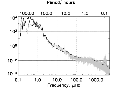
We have applied Fourier and Morlet wavelet transforms to the data. Both gave essentially the same results (see Fig. 1), except that the global wavelet power spectrum shows smaller fluctuations due to the smoothing introduced by Morlet wavelets. The peak in the power at about 5 minutes is due to low degree p-modes, eigen oscillations of the Sun. VIRGO data sampled every minute or every hour (not shown in the figure) display enhanced power at frequencies above 5 $\mu$Hz relative to SORCE/TIM data. This enhancement of power in the VIRGO data is due to noise in the electronic calibration. This noise is roughly constant at a level of 50 ppm at low frequency, but drops at higher frequencies, having its 3-db point at around 10 $\mu$Hz, which makes it appear as a bump in the solar spectrum (C. Fröhlich 2008, priv. comm.). Differences between VIRGO and TIM data at frequencies below 1 $\mu$Hz are due to the different times they refer to (2002 for VIRGO and 2003 for TIM).

Figure 2: Ratio of wavelet global power spectra of activity maximum to those at activity minimum for the TSI (solid line) and three VIRGO channels: red (dot-dashed line), green (dashed) and blue (dotted).

In order to estimate the time scale at which the relative contribution of magnetic field evolution (which is solar cycle phase dependent) and of convection (which is almost independent) becomes equal, we have analyzed VIRGO records for quiet (1996–1997) and active (1999–2000) Sun periods individually. For the component related to active region magnetic fields we expect stronger variations at activity maximum than at minimum.

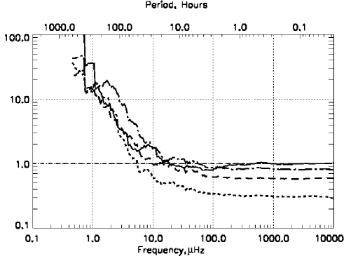
The ratio of the wavelet power spectrum of the 1999–2000 period to that of 1996–1997 is shown in Fig. 2. The ratio exceeds unity at periods longer than a day. Obviously at these periods magnetic fields dominate the variability. At shorter periods, the ratio is essentially 1 in the total irradiance. Values below 1 are seen in the 3 color channels. They may be an instrumental artifact, although the reason has not been identified (C. Fröhlich 2003, priv. comm.). Fröhlich & Lean (2004) employed the data between 2000.8 and 2002.8 for the active period to arrive at a value somewhat higher than 1. Since the Sun was more active during this latter period than during 1999–2000, this may partly explain the higher value. They have also apparently used a later version of the SPM data. From this diagram alone it is not possible to say whether there is a non-magnetic source of the irradiance variations above 10 $\mu$Hz, e.g. convection, or a magnetic source, e.g. the network, which does not change strongly in strength over the solar cycle (Harvey 1994). At frequencies between approximately 10 and 100 $\mu$Hz (which are of particular interest for planetary transits and g-mode search) both magnetic field and convection may contribute to the power.

3 Short term variability: Granulation model

3.1 Description of the Model

To extrapolate from the Sun to other stars it is necessary to construct models that are easily scalable to other stars. Here we concentrate on convection. Of the main scales of solar convection, there is no evidence that the larger scales (meso- and supergranulation) show any intrinsic brightness contrast after the contribution from magnetic fields is eliminated. Mesogranular structure is best visible when following ‘corks’ over an hour or two (November & Simon, 1988; November, 1989) or when considering the spatial distribution of, e.g., exploding granules (Roudier & Muller, 1987; Ploner et al., 2000). There is no evidence that they show any intrinsic brightness contrast (cf. Straus & Bonaccini, 1997; Hathaway et al., 2000; Rieutord et al., 2000; Roudier et al., 2009). Supergranulation is mainly evident in intensity images that sample wavelengths at which small-scale magnetic elements are bright (e.g., Solanki, 1993). Rast (2003) has set tight limits on the visible contrast between supergranule cell interior and boundaries if the magnetic features are masked out. If correct, any significant contribution to irradiance variations produced by a supergranule must come from the evolution of the magnetic field at its boundary. We therefore concentrate here on modelling the granulation and deal separately with the magnetic field (Sect. 4).

Figure 3: Normalized distributions: a) granule lifetimes; b) granule sizes. Plotted is a snapshot at a moment of the evolution. Dashed lines give observed distributions, solid lines the distributions in the ‘standard’ model.

To model the influence of the roughly $10^{6}$ granules on the solar disk, we use a simple parameterized description of individual granules and a statistical approach to the evolution of the whole ensemble. Each granule is treated as a brightness structure, with a time-dependent bright part (granule) that is assigned a brightness value and area and a dark part (intergranular lane), whose brightness is fixed and does not change with time. The granule distribution and evolution are determined by the following free parameters: the granule expansion or contraction rate, the granule lifetime, rate of brightness increase or decrease, ratio of the splitting granules to ones that dissolve.

The key features of our model are: 1) The main birth and death mechanisms of granules are fragmentation (birth and death) and emergence from (birth), or dissolution into (death) the background (e.g., Mehltretter, 1978; Kawaguchi, 1980; Hirzberger et al., 1999). 2) The brightness value of each granule is assigned randomly within a given range. 3) The lifetime distribution of all granules follows an exponential law (Fig. 3a). For the models designated as the ‘standard’ model the lifetime distribution follows the one derived empirically by Hirzberger et al. (1999) with the decay time of $\tau=4.68$ minutes. 4) The initial distribution of granule sizes in the standard model is described by the best fit exponential function to the observed distribution published by Roudier & Muller (1987). The observed distribution is represented by the dashed line in Fig. 3b.

While granules evolve their size changes such that larger granules expand and smaller ones shrink. Due to the excess pressure large granules build up in the photosphere relative to their neighbors (e.g., Ploner et al., 1999). At the end of its life, depending on its size, each granule can either split into two parts, thus forming 2 new granules, or dissolve into the background. The end of a granule’s life is reached either when the preassigned time (lifetime) has run out or when its size reaches the limits of the size distribution. The rate at which the granule’s size changes grows linearly from 0 in the middle of the size distribution to the maximum of 0.1 arcsecond per minute at the lowest and highest diameter distribution edges. This effectively means that the smaller the granule the faster it is squeezed out of existence by its neighbors, and the bigger the granule the faster it reaches the upper size limit imposed in this model and splits into two parts. The individual areas of the child granules lie randomly between 1/4 and 3/4 of the area of the parent granule.

We attempt to reduce sudden jumps in the brightness at the time of death or birth of a granule (which produce artificial high-frequency power). Thus the brightness of granules born out of the splitting of a larger granule slightly increases, in order to compensate for the increased area of the intergranular network, which after splitting surrounds 2 granules instead of one before splitting. Small granules that are close to disappearing or have just been born have brightness levels close to the background intergranular lanes. Such transitions are linear and limited in time: brightness drops or rises are completed in 3 minutes. The total number of granules is kept constant by maintaining a balance between appearing and dying granules. Also, the size distribution is roughly maintained by allowing fresh granules with the appropriate size distribution to emerge from the intergranular lanes. In Fig. 3b we plot the empirical size distribution of granules (dashed curve), which is very close to the initial size distribution. The solid line represents the size distribution of the synthetic granules at a typical later time. The output irradiance of the model is normalized by the total area of the sun at each time step.

In order to check the importance of model parameters, we have varied each of them individually, while keeping the rest fixed. The results of this parameter study are presented in Sect. 3.2. Two other parameters, the total number of granules, $N_{tot}$, and the average brightness contrast between granules and intergranular lanes move the irradiance power spectrum up or down, but do not influence its slope. They are therefore not discussed further here.

Figure 4: Wavelet power spectra (in ppm${}^{2}/60\leavevmode\nobreak\ \mu$Hz) for different granule lifetimes. Solid line shows the result based on the solar lifetime distribution with a mean lifetime of $\sim$5.2 min.; dotted line is for longer lifetimes with a mean of $\sim$23.7 min. and dashed line for shorter lifetimes with a mean of $\sim$2.9 min.

3.2 Results

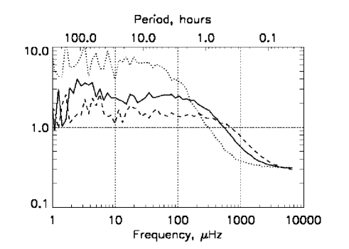
Power spectra from a parameter study carried out with our model are shown in Figs. 4 and 5. Except for the parameter explicitly mentioned in each case, all others remain unchanged at their standard values: mean granule lifetime is approximately 5 minutes, mean granule diameter is approximately 0.9 arcseconds.

At low frequencies all model power spectra are relatively independent of frequency (but with increasing fluctuations towards lower frequency due to the fewer periods of this length sampled by the simulation). Above a certain frequency the power drops approximately as a power law. The flattening of the power spectrum at higher frequencies is due to aliasing introduced by the fact that granules evolve also on periods shorter than the employed time step (1 minute); imposed by the typically 6 months solar time that a model has to be run in order to obtain reliable results also at lower frequencies.

The curves in Fig. 4 refer to different average granule lifetimes. As expected, the frequency at which the power starts to decrease (i.e. the ‘knee’ in the wavelet power spectrum) increases with decreasing lifetime of granules. The corresponding period roughly doubles as the average granule lifetime is doubled, so that this parameter is potentially a diagnostic of stellar granule lifetimes. Note, however, that the period of the ‘knee’ is roughly 10 times longer than the average granule lifetime.

Figure 5: Wavelet power spectra (in ppm${}^{2}/60\leavevmode\nobreak\ \mu$Hz) for different granule sizes (solid line: maximum diameter of a granule is 3 arcsec, dotted line: maximum diameter is 9 arcsec, dashed line: maximum diameter 2 arcsec).

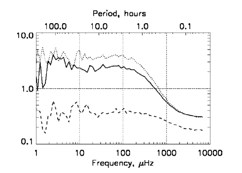
In Fig. 5 the diameter of granules has been varied. The number of granules is kept constant, so that the total area covered is larger in the case of larger granules (corresponding to a bigger star). Obviously small granules produce less noise than big ones with a shallower slope of the power below several hours. This is caused by the fact that the ratio of the granule area to that of the surrounding intergranular lanes is higher for big granules; the ratio grows with granular diameter because the width of the intergranular lanes is fixed. Hence the ratio grows almost like the ratio of area to circumference, i.e. nearly linearly with granule diameter. Changing the width of the intergranular lanes while keeping the size distribution fixed gives basically the same result.

Note that changing a single parameter can lead to subtle indirect changes in the properties of the ensemble of granules and hence of the wavelet power spectrum. As an example, a change in the size distribution of granules also leads to a change of their effective lifetime distribution. Thus for a very small average granule size more granules die early by reaching the limits of the size distribution. For a star of constant size the number of granules is reduced if the average granule size is bigger. Therefore the curves in Fig. 5 would lie even further apart for a fixed stellar surface area. The dotted line would lie higher by a factor of approximately $\sqrt{3}$, while the dashed line would move down by the same factor. We also found that splitting granules on the stellar surface produce higher levels of noise than dissolving granules. This is partly due to the fact that splitting granules are on average bigger, so that a similar picture emerges as shown in Fig. 5 (with some differences, since the shape of the lifetime and size distributions change significantly with the ratio of splitting to dissolving granules).

4 Magnetic field contribution to irradiance variations

Here we employ the SATIRE-S (Spectral And Total Irradiance REconstruction for the Satellite era; Fligge et al., 2000; Krivova et al., 2003; Solanki et al., 2005; Krivova et al., 2011) model, which is based on the assumption that all irradiance changes on timescales of days to years are entirely due to the evolution of the magnetic flux on the solar surface and includes four components of the solar photosphere: quiet Sun (solar surface free of magnetic fields), umbra and penumbra of sunspots, as well as bright magnetic features forming faculae and the network (described as a single component). Calculation of solar irradiance requires two input data sets. The first one is the intensities of each atmospheric component as a function of the wavelength and of the angle between the line of sight and the normal to the solar surface (i.e. the center-to-limb variation). These time-independent spectra are taken from Unruh et al. (1999). The second data set is composed of the maps describing the distribution of the magnetic features (umbrae, penumbrae, plage and faculae) on the solar surface at a given time. They are produced from magnetograms and continuum images (see Krivova et al. 2003 for details) recorded by MDI on board SOHO (Scherrer et al. 1995). The changing area coverage and distribution of the different components introduces the time variability of the brightness.

Usually, MDI does not record continuum images and full-disk magnetograms with the necessary low noise level (5-min integration, corresponding to a noise level of 9 G) at the cadence required for the present investigation. However, we found a 2.2-month period from 15th of March to 19th of May 1999 when MDI magnetograms were recorded at a rate of at least one 5-min sequence every half an hour practically without interruptions. Unfortunately, the continuum images, required to determine umbral and penumbral area, were recorded with a cadence of only 96 minutes over the same period of time. Therefore, every continuum image is used for 3 points in time by rotating it to the times of the corresponding magnetograms. Since sunspots can evolve over this interval, the obtained power at periods of a few hours is probably somewhat underestimated.

SATIRE-S has a single free parameter, $B_{sat}$, which enters in how the magnetogram signal in facular and network regions is converted into brightness. It is described in detail by, e.g., Fligge et al. (2000); Krivova et al. (2003); Wenzler et al. (2006). Here we adopt the value of $B_{sat}$=280 G following Krivova et al. (2003).

The time series produced in this manner is plotted in Fig. 6 (lower black curve). Compared with the irradiance fluctuations measured by VIRGO (top curve in Fig. 6) the irradiance variations induced by the magnetic field follow the longer term variations very well, but are too smooth, i.e. they obviously lack power at very short periods. Some artifacts (small brightening spikes) are seen at selected times between days 5 and 11. They are due to artifacts in some of the images recorded on these days. The power spectrum resulting from this reconstruction is represented by the dotted line in Fig. 7 (between about 1 and 250$\mu$Hz).

5 Combined short and long time scale variability

Figure 6: Total solar irradiance observed by VIRGO between March and May 1999 (upper black curve) and reconstructed using MDI data (lower black curve). Also plotted (in gray) is the combination of magnetic reconstruction with granulation model. The sampling rate of the VIRGO data is 1 minute, while the magnetic reconstruction alone is sampled each 30 minutes. The magnetic reconstruction and the combined reconstruction plus granulation model are shifted down by 500 ppm to facilitate the visual comparison.

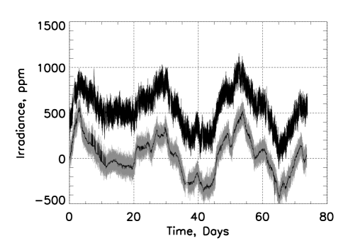
Now we have 2 parts of the solar irradiance — one is reconstructed using only the magnetic activity of the Sun, the other is based exclusively on the convective ‘noise’ of the solar surface, i.e. caused only by granulation. In order to compare modelled variability and observed one, we combine both magnetic and granulation parts. The granulation model used here is the ‘standard’ model with granule parameters based on observed solar values (see Sect. 3.1 for a description). It corresponds to the solid curves in Figs. 4 and 5. Both models were run for the same length of time here, namely 2.2 months. To combine magnetic reconstructions with granulation model results we re-sample magnetic reconstructions from 30 minutes down to a 1 minute sampling rate. As seen in Fig. 6, the combined model (gray curve) follows very closely the observed one.

Figure 7: Wavelet power spectra (in ppm${}^{2}/60\leavevmode\nobreak\ \mu$Hz). Thick solid line: VIRGO data set (same as dotted line in Fig. 1). Thin solid line: power spectrum of the granulation model, dotted line: magnetic reconstruction with 30 minutes sampling, dashed line in the left part of the plot: daily sampled magnetic reconstruction.

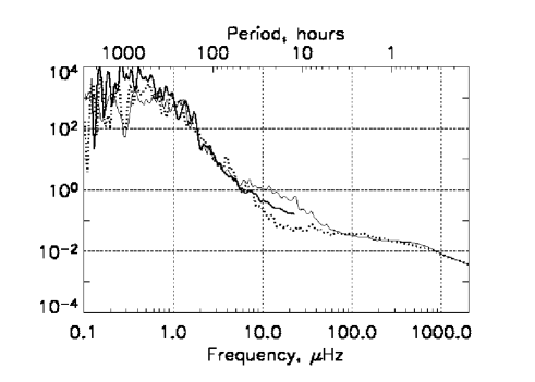
Power spectra of the modelled and observed irradiance allow a more detailed comparison. Figure 7 shows the wavelet power spectra of the observed data (thick solid line), of the irradiance produced by the granulation model (high frequencies; thin solid line) and the magnetic field model (frequencies $\approx 1-250\mu$Hz; dotted line). Since half-hourly sampled magnetograms are available only for 2.2 months, while the diagram covers 4 months (and VIRGO data allow even longer periods to be considered), we have also employed the reconstruction carried out by Krivova et al. (2003) which is sampled at a cadence of 1 day and represented by the dashed line in the left part of Fig. 7. The low frequency part, caused exclusively by the magnetic activity, is in good agreement with the observed spectrum. The high frequency part obtained using the solar surface granulation model (now run for a larger number of granules) recreates real power rather well at frequencies above 100 $\mu$Hz and gives a negligible contribution to the combined irradiance at frequencies below 10 $\mu$Hz. Figure 7 confirms that the solar total irradiance noise background is equally determined by convection (granulation) and magnetism at periods of 10 hours (cf. Fig. 2).

In order to compare the observed and modelled power spectra in more detail, we combine all 3 components of the model. Figure 8 shows wavelet power spectra of the observed VIRGO (thin solid line) and SORCE data (thick solid line) and of the reconstructed irradiance (dotted) produced by combining the various reconstructions plotted in Fig. 7. SORCE data are for the year 2003 and sampled every 6 hours, while the employed VIRGO data are sampled each minute and refer to 2002. The comparison with the SORCE spectrum confirms that the VIRGO power enhancement in the band from 7 to 30 $\mu$Hz is an artifact (C. Fröhlich, priv. comm.). The different years to which the SORCE TIM and VIRGO data refer to should not affect this result, since variability at 10–100 $\mu$Hz is hardly affected by solar cycle phase (see Fig. 2). Note, however, that the modelled variability lies below both VIRGO and SORCE TIM measurements in the frequency range 8–70 $\mu$Hz.

Figure 8: Wavelet power spectra (in ppm${}^{2}/60\leavevmode\nobreak\ \mu$Hz). Thin solid line: VIRGO data set. Dotted line: power spectrum of the combined magnetic reconstruction and granulation model. Thick solid line: SORCE wavelet power spectrum.

6 Conclusions

We have analyzed solar irradiance variations on time scales between minutes and months. Whereas on time scales of a day and longer, the main mechanism of variations is the evolution of the solar magnetic field, on time scales shorter than roughly half a day granular convection becomes dominant. The crossover between magnetic and convective signatures coincides with the frequency band of most interest for planetary transit observations.

If we neglect the 5-min band, then results of combined modelling of irradiance variations due to granular convection and surface magnetism suggest that we are able to reproduce solar irradiance variability using only data of magnetic activity on the surface of the Sun and ‘noise’ produced by granulation, except for periods between 5 and 30 hours. In this range of periods the solar variability is underestimated by the model by up to a factor of 5 when comparing with VIRGO TSI and up to a factor of 2 when comparing with SORCE TIM. Due to the influence of electronic noise on the VIRGO data, we believe the latter ratio is the more reliable one. The discrepancy may have one of the following causes: 1. The lack of larger scales of convection, such as supergranulation (and possibly mesogranulation) in the model. 2. Insufficient sensitivity of MDI magnetograms to weak fields (i.e. to quiet Sun fields) and therefore also to their variability. 3. Insufficient spatial resolution of the magnetograms, so that flux with mixed polarities at small spatial scales, as is typical of the quiet Sun, can be missed (Krivova & Solanki, 2004). 4. The breakdown of one of the assumptions underlying the magnetic field-based reconstructions. For example, the simplifying assumption that all magnetic features at a certain limb distance and a given magnetic flux have the same brightness is expected to break down at some level. 5. The high frequency component of the evolution of sunspots and pores is inaccurately represented by the interpolation between the continuum images separated by 96 minutes. The Nyquist frequency of this data set lies at 45 $\mu$Hz, making this explanation less likely. Note that the time-scale on which the quiet Sun network flux is replaced by ephemeral regions, 14 hours according to Hagenaar (2001), falls in the critical time range and supports causes 2 and 3 above.

The present investigation also provides an evaluation of the diagnostic potential of power spectra of radiative flux time series for determining the properties of stellargranulation. Granule contrasts, the number of granules, granule lifetimes and diameters, as well as contrast and thickness of intergranular lanes are important factors determining the amplitude and the shape of the power spectrum at periods shorter than several hours. In particular, power spectra, such as those that can be obtained from COROT (Baglin et al., 2002) and Kepler (Borucki et al., 2003) data, allow granule lifetimes to be determined in a relatively unique manner. This is of some interest, since traditional techniques for diagnosing stellar granulation, such as line bisectors, do not provide any information on granule lifetimes. Note that this diagnostic is not affected by any uncertainties in the model below 100 $\mu$Hz.

Important next steps are to identify the source of the missing power around periods of 10–20 hours and to extend such an analysis to other stars with different effective temperatures and gravities, as well as with different rotation rates and magnetic activity levels. Magnetograms and continuum images obtained at high cadence by the HMI instrument on SDO could play a prominent role in the former exercise.