Linear-Response Dynamics from the Time-Dependent Gutzwiller Approximation

Abstract

Within a Lagrangian formalism we derive the time-dependent Gutzwiller approximation for general multi-band Hubbard models. Our approach explicitly incorporates the coupling between time-dependent variational parameters and a time-dependent density matrix from which we obtain dynamical correlation functions in the linear response regime. Our results are illustrated for the one-band model where we show that the interacting system can be mapped to an effective problem of fermionic quasiparticles coupled to “doublon” (double occupancy) bosonic fluctuations. The latter have an energy on the scale of the on-site Hubbard repulsion $U$ in the dilute limit but becomes soft at the Brinkman-Rice transition which is shown to be related to an emerging conservation law of doublon charge and the associated gauge invariance. Coupling with the boson mode produces structure in the charge response and we find that a similar structure appears in dynamical mean-field theory.

1 Introduction

Recent advances in ultra-fast spectroscopy allow us to monitor the dynamics of electrons on a femtosecond scale. This is especially interesting for strongly correlated materials, such as high-temperature superconductors [1, 2, 3], since in their case the spectroscopic probe is able to investigate the intra-electronic redistribution of excitation energies before the relaxation via the lattice starts. From the theoretical point of view, this is obviously a challenging problem since it requires a method capable of treating the relaxation dynamics of a strongly correlated system out of equilibrium. In this regard, a state-of-the art approach is the dynamical mean-field theory (DMFT) which has recently been applied [4] to the single-band Hubbard model in order to study the double-occupancy relaxation after laser excitation. However, for the application to real systems this method is rather demanding from a numerical point of view since it requires the self-consistent solution of complex single-impurity models driven out of equilibrium.

In this regard, the time-dependent Gutzwiller approximation (TDGA) is a promising alternative since it joins the numerical simplicity of standard random phase approximation (RPA) with the ability to capture important many-particle effects, as the Mott-Hubbard transition. In a series of papers [5, 6, 7, 8], we have developed the TDGA which is based on a variational Ansatz for the Hubbard model [9, 10] evaluated in the limit of infinite spatial dimensions [11]. This approach has recently been generalised for the study of multi-band Hubbard models [12, 13] and is based on the expansion of the Gutzwiller energy functionals which depend on the density matrix and variational parameters related to the atomic eigenstates. In previous work [5, 6] the latter have been eliminated by assuming that they instantaneously adjust to the density fluctuations (‘antiadiabaticity approximation’). As a result, one obtains an energy functional which only depends on the density matrix and therefore the RPA for density-dependent forces [14, 15] can be applied in order to evaluate response functions. This (approximate) version of the TDGA has been applied successfully to the evaluation of dynamical correlation functions in cuprate superconductors [16] including the optical conductivity [17] and the magnetic susceptibility [18, 19]. It has also been related to Auger spectroscopy by calculating pair excitations in one- [8] and three-band [20] Hubbard models.

More recently the TDGA was extended by Schiró and Fabrizio [21, 22, 23] towards the inclusion of time-dependent variational parameters. Concerning the evaluation of response functions this approach can supersede the ‘antiadiabaticity assumption’, mentioned above, since the double-occupancy dynamics follows from a time-dependent variational principle. However, in Refs. [21, 22] the authors focused on the study of quantum quenches for systems with a homogeneous ground state. In this case, the time dependence is captured by the double-occupancy dynamics whereas the single-particle density matrix is time-independent. Recent developments consider simultaneously the dynamics of the double occupancy and of the density matrix [24, 25].

In this paper we will re-derive the TDGA for a time-dependent Gutzwiller variational wave-function applied to multi-band Hubbard models. Our resulting equations of motion will explicitly capture the coupling between the time-dependent variational parameters and the density matrix. We will analyse these equations in the small-amplitude (i.e., linear response) limit and apply the theory to the evaluation of dynamical charge correlations in the single-band case. It turns out that the previous formulation of the TDGA [5, 6] is recovered in the low-frequency limit. However, the incorporation of fluctuations in the time-dependent density of double occupied states (“doublons”) leads to additional spectral weight above the band-like excitations in very good agreement with exact diagonalisation and DMFT.

The paper is organised as follows: In Sec. 2.1 we introduce the time-dependent variational principle which is underlying the present work. Since the corresponding expectation values are evaluated with multi-band Gutzwiller wave-functions the latter are presented in Sec. 2.2. The evaluation of time-dependent matrix elements is performed in Sec. 2.3 which allows for the derivation of the Lagrangian and corresponding equations of motion in Sec. 2.4. Our investigations are specified for the single-band Hubbard model in Sec. 3, where we also discuss a two-site example which can be treated analytically. Finally, the small amplitude limit of the TDGA is derived in Sec. 4 and discussed in the context of response functions in Sec. 5. Numerical results for the dynamical charge susceptibility are presented in Sec. 6 and compared with dynamical mean-field theory (DMFT) and exact diagonalisation. We finally conclude our investigations in Sec. 7.

2 The time-dependent Gutzwiller theory

2.1 Variational Principle

The time-dependent Schrödinger equation for a general time-dependent Hamiltonian $\hat{H}(t)$ ($\hbar=1$), can be obtained by requesting that the action

$$S=\int dtL(t)$$ (1)

is stationary with respect to variations of the wave function. It is in general convenient to perform this variation based on a real Lagrangian [26]

$$L(t)=\frac{\rmi}{2}\frac{\langle\Psi|\dot{\Psi}\rangle-\langle\dot{\Psi}|\Psi\rangle}{\langle\Psi|\Psi\rangle}-\rmi\frac{\langle\Psi|\hat{H}|\Psi\rangle}{\langle\Psi|\Psi\rangle}\;,$$ (2)

which leads to equations of motion that are independent of the phase and the norm of the wave-functions.

If one restricts the wave-function $\left|\Psi(z_{i}(t))\right\rangle$ to a certain trial form, depending on a set of (in general complex) ‘variational parameters’ $z_{i}(t)$, the Euler-Lagrange equations for $z_{i}(t)$ provide an approximation for the time evolution of the system. For example, restricting the wave-function to Slater determinants and using the amplitude of the single particle orbitals as variational parameters yields the time-dependent Hartree-Fock approximation. In this work, we will consider variational wave functions of the Gutzwiller form [9, 10, 11] for general multi-band Hubbard models leading to the time-dependent Gutzwiller approximation.

2.2 Gutzwiller energy functionals for multi-band Hubbard models

We first recall some results of the conventional Gutzwiller approximation for the ground state properties of multi-band systems. We aim to study the physics of the following family of models,

$$\hat{H}=\sum_{i\neq j}\sum_{\sigma,\sigma^{\prime}}t^{\sigma,\sigma^{\prime}}_{i,j}\hat{c}^{\dagger}_{i,\sigma}\hat{c}^{\phantom{\dagger}}_{j,\sigma^{\prime}}+\sum_{i}\hat{H}_{i,{\rm loc}}\;,$$ (3)

where $t^{\sigma,\sigma^{\prime}}_{i,j}$ denotes the ‘hopping parameters’ and the operators $\hat{c}^{(\dagger)}_{i,\sigma}$ annihilate (create) an electron with spin-orbital index $\sigma$ on a lattice site $i$. The local Hamiltonian

$$\hat{H}_{i;{\rm loc}} = \sum_{\sigma_{1},\sigma_{2}}\varepsilon_{i;\sigma_{1},\sigma_{2}}\hat{c}^{\dagger}_{i,\sigma_{1}}\hat{c}^{\phantom{\dagger}}_{i,\sigma_{2}}$$

$$+\sum_{\sigma_{1},\sigma_{2},\sigma_{3},\sigma_{4}}U_{i}^{\sigma_{1},\sigma_{2},\sigma_{3},\sigma_{4}}\hat{c}^{\dagger}_{i,\sigma_{1}}\hat{c}^{\dagger}_{i,\sigma_{2}}\hat{c}^{\phantom{\dagger}}_{i,\sigma_{3}}\hat{c}^{\phantom{\dagger}}_{i,\sigma_{4}}\;$$

is determined by the orbital-dependent on-site energies $\varepsilon_{i;\sigma_{1},\sigma_{2}}$ and by the two-particle Coulomb interaction $U_{i}^{\sigma_{1},\sigma_{2},\sigma_{3},\sigma_{4}}$. Upon introducing the eigenstates $\left|\Gamma\right\rangle_{i}$ and eigenvalues $E_{i;\Gamma}$ of  (2.2) (which can be readily calculated by means of standard numerical techniques) the local Hamiltonian can be written as

$$\hat{H}_{i,{\rm loc}} = \sum_{\Gamma}E_{i;\Gamma}|\Gamma\rangle{\phantom{\rangle}}_{i}\hskip 1.42271pt{\phantom{\rangle}}_{i}\langle\hskip 0.85355pt\Gamma^{\prime}|\;.$$ (5)

Multi-band Gutzwiller wave-functions have the form

$$|\Psi_{\rm G}\rangle=\hat{P}_{\rm G}|\Psi_{\rm S}\rangle=\prod_{i}\hat{P}_{i}|\Psi_{\rm S}\rangle\;,$$ (6)

where $|\Psi_{\rm S}\rangle$ is a normalised Slater determinant and the local Gutzwiller correlator is defined as

$$\hat{P}_{i}=\sum_{\Gamma,\Gamma^{\prime}}\lambda_{i;\Gamma,\Gamma^{\prime}}|\Gamma\rangle_{i}{}_{i}\langle\Gamma^{\prime}|\;.$$ (7)

Here we introduced the variational-parameter matrix $\lambda_{i;\Gamma,\Gamma^{\prime}}$ which allows us to optimise the occupation and the form of the eigenstates of $\hat{P}_{i}$.

The evaluation of expectations values with respect to the wave function (6) is a difficult many-particle problem, which cannot be solved in general. As shown in Refs. [27, 28], one can derive analytical expressions for the variational ground-state energy in the limit of infinite spatial dimensions ($D\to\infty$). Using this energy functional for the study of finite-dimensional systems is usually denoted as the ‘Gutzwiller approximation’. This approach is the basis of most applications of Gutzwiller wave functions in studies of real materials and it will also be used in this work. One should keep in mind, however, that the Gutzwiller approximation has its limitations and the study of some phenomena requires an evaluation of expectation values in finite dimensions [29, 30].

For the evaluation of Gutzwiller wave functions in infinite dimensions it is most convenient to impose the following (local) constraints [27, 28]

$$\langle\hat{P}^{\dagger}\hat{P}\rangle_{\Psi_{\rm S}} = 1\;,$$ (8)

$$\langle\hat{P}^{\dagger}\hat{P}\hat{c}^{\dagger}_{\sigma}\ \hat{c}_{\sigma^{\prime}}\rangle_{\Psi_{\rm S}} = \langle\hat{c}^{\dagger}_{\sigma}\hat{c}_{\sigma^{\prime}}\rangle_{\Psi_{\rm S}}\;.~{}$$ (9)

With these constraints, the expectation value of the local Hamiltonian (5) reads

$$\langle\hat{H}_{\rm loc}\rangle_{\Psi_{\rm G}}=\sum_{\Gamma,\Gamma_{1},\Gamma_{2}}E_{\Gamma}\lambda_{\Gamma,\Gamma_{1}}^{*}\lambda_{\Gamma,\Gamma_{2}}m_{\Gamma_{1},\Gamma_{2}}\;,$$ (10)

where

$$m_{\Gamma_{1},\Gamma_{2}}\equiv\langle(|\Gamma_{1}\rangle\langle\Gamma_{2}|)\rangle_{\Psi_{\rm S}}$$ (11)

can be calculated by means of Wick’s theorem.

The expectation value of a hopping operator in infinite dimensions has the form

$$\big{\langle}\hat{c}_{i,\sigma_{1}}^{\dagger}\hat{c}_{j,\sigma_{2}}^{\phantom{+}}\big{\rangle}_{\Psi_{\rm G}}=\sum_{\sigma^{\prime}_{1},\sigma^{\prime}_{2}}q_{\sigma_{1}}^{\sigma^{\prime}_{1}}\left(q_{\sigma_{2}}^{\sigma^{\prime}_{2}}\right)^{*}\big{\langle}\hat{c}_{i,\sigma^{\prime}_{1}}^{\dagger}\hat{c}_{j,\sigma^{\prime}_{2}}^{\phantom{+}}\big{\rangle}_{\Psi_{\rm S}}\;,$$ (12)

where the (local) renormalisation matrix $q_{\sigma}^{\sigma^{\prime}}$ is an analytic function of the variational parameters and of the non-interacting local density matrix

$$C_{i;\sigma,\sigma^{\prime}}=\langle\hat{c}^{\dagger}_{i,\sigma}\hat{c}^{\phantom{\dagger}}_{i,\sigma^{\prime}}\rangle_{\Psi_{\rm S}}\;.$$ (13)

The explicit form of the renormalisation matrix is given, e.g., in Ref. [31] but will not be needed for our further considerations in this work. In the following, we assume that the correlated and the non-correlated local density matrix are equal,

$$C^{\rm c}_{i;\sigma,\sigma^{\prime}}=\langle\hat{c}^{\dagger}_{i,\sigma}\hat{c}^{\phantom{\dagger}}_{i,\sigma^{\prime}}\rangle_{\Psi_{\rm G}}=C_{i;\sigma,\sigma^{\prime}}\;.$$ (14)

This is the case when all non-degenerate orbitals on a lattice site belong to different representations of its point symmetry group.

In summary, the expectation value of the Hamiltonian (3),

$$E^{\rm GA}=E^{\rm GA}(\tilde{\lambda}^{(*)},\tilde{\rho})\;,$$ (15)

is a function of all variational parameters $\tilde{\lambda}^{(*)}\equiv\{\lambda^{(*)}_{i;\Gamma,\Gamma^{\prime}}\}$ and of the non-interacting density matrix $\tilde{\rho}$ with the elements

$$\rho_{(i\sigma),(j\sigma^{\prime})}\equiv\langle\hat{c}_{j,\sigma^{\prime}}^{\dagger}\hat{c}_{i,\sigma}^{\phantom{+}}\rangle_{\Psi_{\rm S}}\;.$$ (16)

The same holds for the constraints (8), (9), for which we will use the abbreviation

$$g_{n}(\tilde{\lambda}^{(*)},\tilde{\rho}))=0\;\;\;,\;\;\;1\leq n\leq n_{\rm c}$$ (17)

where $n_{\rm c}$ is the maximum number of independent constraints. In Sec. 3 we apply these results to the special case of a single-band Hubbard model.

2.3 Evaluation of time-dependent matrix elements

In this section, we will apply the concept, introduced in Sec. 2.1, to the general class of Gutzwiller wave functions

$$|\Psi_{\rm G}(t)\rangle=\hat{P}_{\rm G}(t)|\Psi_{\rm S}(t)\rangle=\prod_{i}\hat{P}_{i}(t)|\Psi_{\rm S}(t)\rangle\;,$$ (18)

where the single-particle product states $\left|\Psi_{\rm S}(t)\right\rangle$ and the local correlation operators

$$\hat{P}_{i}(t)=\sum_{\Gamma,\Gamma^{\prime}}\lambda_{i;\Gamma,\Gamma^{\prime}}(t)|\Gamma\rangle_{i}{}_{i}\langle\Gamma^{\prime}|$$ (19)

are now time-dependent quantities.

The state $|\Psi_{\rm S}(t)\rangle$ can be written as

$$|\Psi_{\rm S}(t)\rangle=\prod_{\gamma}[\hat{h}^{\dagger}_{\gamma}(t)]^{n_{\gamma}}\left|\rm vac\right\rangle\;.$$ (20)

Here, $n_{\gamma}\in(0,1)$ determines which of the single particle states $\left|\gamma(t)\right\rangle$, described by the operators

$$\hat{h}^{\dagger}_{\gamma}(t)=\sum_{\upsilon}u_{\upsilon,\gamma}(t)\hat{c}^{\dagger}_{\upsilon}\;,$$ (21)

are occupied and $u_{\upsilon,\gamma}(t)$ is a (time-dependent) unitary transformation,

$$\sum_{\gamma}u_{\upsilon_{1},\gamma}^{*}(t)u_{\upsilon_{2},\gamma}(t)=\delta_{\upsilon_{1},\upsilon_{2}}\;.$$ (22)

The functions $u_{\upsilon,\gamma}$ constitute a second set of (time-dependent) variational parameters (in addition to $\lambda_{i;\Gamma,\Gamma^{\prime}}(t)$) and determine the single-particle wave function $|\Psi_{\rm S}\rangle$. Note that the time dependence of the operators (21) implies that the non-interacting density matrix

$$\rho_{\upsilon,\upsilon^{\prime}}(t)=\langle\hat{c}^{\dagger}_{\upsilon^{\prime}}\hat{c}_{\upsilon}\rangle_{\Psi_{\rm S}(t)}=\sum_{\gamma}n_{\gamma}u^{*}_{\upsilon^{\prime},\gamma}(t)u_{\upsilon,\gamma}(t)$$ (23)

is also time dependent.

We start with a consideration of the time derivative in Eq. (2) which requires the evaluation of

$$\frac{\langle\Psi_{\rm G}|\dot{\Psi}_{\rm G}\rangle}{{\langle\Psi_{\rm G}|\Psi_{\rm G}\rangle}}=\frac{\langle\Psi_{\rm S}|\hat{P}^{\dagger}_{\rm G}\hat{P}_{\rm G}|\dot{\Psi}_{\rm S}\rangle}{\langle\Psi_{\rm S}|\hat{P}^{\dagger}_{\rm G}\hat{P}_{\rm G}|\Psi_{\rm S}\rangle}+\frac{\langle\Psi_{\rm S}|\hat{P}^{\dagger}_{\rm G}\dot{\hat{P}}_{\rm G}|\Psi_{\rm S}\rangle}{\langle\Psi_{\rm S}|\hat{P}^{\dagger}_{\rm G}\hat{P}_{\rm G}|\Psi_{\rm S}\rangle}$$ (24)

and its complex conjugate. With Eqs. (20) and (21), we find

$$|\dot{\Psi}_{\rm S}\rangle = \sum_{\gamma}\dot{\hat{h}}^{\dagger}_{\gamma}\hat{h}_{\gamma}|\Psi_{\rm S}\rangle$$ (25)

$$= \sum_{\upsilon}\sum_{\gamma,\gamma^{\prime}}\dot{u}_{\upsilon,\gamma}u^{*}_{\upsilon,\gamma^{\prime}}\hat{h}^{\dagger}_{\gamma^{\prime}}\hat{h}_{\gamma}|\Psi_{\rm S}\rangle\;.$$ (26)

This equation allows us to evaluate the contribution of the first term on the r.h.s. of Eq. (24) as

$$\frac{\langle\Psi_{\rm S}|\hat{P}^{\dagger}_{\rm G}\hat{P}_{\rm G}|\dot{\Psi}_{\rm S}\rangle}{\langle\Psi_{\rm S}|\hat{P}^{\dagger}_{\rm G}\hat{P}_{\rm G}|\Psi_{\rm S}\rangle}$$

$$=\sum_{\upsilon}\sum_{\gamma,\gamma^{\prime}}\dot{u}_{\upsilon,\gamma}u^{*}_{\upsilon,\gamma^{\prime}}\frac{\langle\Psi_{\rm S}|\hat{P}^{\dagger}_{\rm G}\hat{P}_{\rm G}\hat{h}^{\dagger}_{\gamma^{\prime}}\hat{h}_{\gamma}|\Psi_{\rm S}\rangle}{\langle\Psi_{\rm S}|\hat{P}^{\dagger}_{\rm G}\hat{P}_{\rm G}|\Psi_{\rm S}\rangle}$$ (27)

$$=\sum_{\upsilon,\gamma}n_{\gamma}\dot{u}_{\upsilon,\gamma}u^{*}_{\upsilon,\gamma}\;.$$ (28)

In the last line, we have used that, in all relevant applications, $\hat{P}_{\rm G}$ and $|\Psi_{\rm S}\rangle$ have the same symmetry and, therefore, all contributions with $\gamma\neq\gamma^{\prime}$ vanish in (27).

We now proceed with a consideration of the second term on the r.h.s. of Eq. (24). With the definition of the correlation operator $\hat{P}_{G}$ we find

$$\langle\Psi_{\rm S}|\hat{P}^{\dagger}_{\rm G}\dot{\hat{P}}_{\rm G}|\Psi_{\rm S}\rangle=\sum_{i}\Big{\langle}\Psi_{\rm S}\Big{|}\Big{(}\prod_{j(\neq i)}\hat{P}^{\dagger}_{j}\hat{P}_{j}\Big{)}\hat{P}^{\dagger}_{i}\dot{\hat{P}}_{i}\Big{|}\Psi_{\rm S}\Big{\rangle}\;.$$ (29)

The r.h.s. of (29) can be evaluated by the standard diagrammatic techniques in infinite dimensions [27]. This leads to

$$\frac{\langle\Psi_{\rm S}|\hat{P}^{\dagger}_{\rm G}\dot{\hat{P}}_{\rm G}|\Psi_{\rm S}\rangle}{\langle\Psi_{\rm S}|\hat{P}^{\dagger}_{\rm G}\hat{P}_{\rm G}|\Psi_{\rm S}\rangle}=\sum_{i}\langle\Psi_{\rm S}|\hat{P}^{\dagger}_{i}\dot{\hat{P}}_{i}|\Psi_{\rm S}\rangle$$

$$\,\,\,\,\,\,=\sum_{i}\sum_{\Gamma_{1},\Gamma_{2},\Gamma_{3}}\lambda^{*}_{i;\Gamma_{1},\Gamma_{2}}\dot{\lambda}_{i;\Gamma_{1},\Gamma_{3}}m_{i;\Gamma_{2},\Gamma_{3}}\;,$$ (30)

where $m_{i;\Gamma_{2},\Gamma_{3}}=m_{i;\Gamma_{2},\Gamma_{3}}(t)$, as defined in Eq. (11), depends on the local elements of the density matrix (23).

2.4 Lagrangian and equations of motion

From Eqs. (27),(30), together with the expectation value of the Gutzwiller energy derived in Sec. 2.2, we are now in the position to derive the Lagrangian Eq. (2). However, we also need to include two sets of constraints, (i) the unitarity of $u_{\upsilon,\gamma}$ and (ii) the Gutzwiller constraints (17). Therefore we finally obtain the following Lagrangian

$$L = \frac{\rmi}{2}\sum_{i}\sum_{\Gamma_{1},\Gamma_{2},\Gamma_{3}}\left[\lambda^{*}_{i;\Gamma_{1},\Gamma_{2}}\dot{\lambda}_{i;\Gamma_{1},\Gamma_{3}}-\dot{\lambda}^{*}_{i;\Gamma_{1},\Gamma_{2}}{\lambda}_{i;\Gamma_{1},\Gamma_{3}}\right]m_{i;\Gamma_{2},\Gamma_{3}}$$

$$+ \frac{\rmi}{2}\sum_{\upsilon,\gamma}n_{\gamma}\left[\dot{u}_{\upsilon,\gamma}u^{*}_{\upsilon,\gamma}-{u}_{\upsilon,\gamma}\dot{u}^{*}_{\upsilon,\gamma}\right]-E^{\rm GA}(\tilde{\lambda}^{(*)},\tilde{\rho})$$

$$- \sum_{\upsilon,\gamma,\gamma^{\prime}}\Omega_{\gamma,\gamma^{\prime}}(t)(u^{*}_{\upsilon,\gamma}u_{\upsilon,\gamma^{\prime}}-1)-\sum_{n}\Lambda_{n}(t)g_{n}({\lambda}^{(*)},u^{(*)}_{\upsilon,\gamma})$$

where $\Lambda_{n}(t)$ and $\Omega_{\gamma,\gamma^{\prime}}(t)$ are (real) Lagrange-parameters. As will be exemplified below in the single-band case, the original Hamiltonian can be time dependent which will reflect in a time dependence of $E^{\rm GA}$ and allows for a coupling with arbitrary external fields.

From Eq. (2.4) the Euler-Lagrange equations can now be derived in the standard way. The equation for the variational parameters $u^{*}_{\upsilon,\gamma}$ reads

$$-\rmi\dot{u}_{\upsilon,\gamma}+\frac{\partial}{\partial u^{*}_{\upsilon,\gamma}}\left(E^{\rm GA}+V^{\rm GA}_{t}+V^{\lambda}+\sum_{n}\Lambda_{n}g_{n}\right)+\sum_{\upsilon_{2}}\Omega_{\upsilon,\upsilon_{2}}u_{\upsilon_{2},\gamma}=0$$ (32)

which in terms of the density matrix (23) can be rewritten as

$$\rmi\dot{\tilde{\rho}}=[\tilde{h}^{\rm GA},\tilde{\rho}]\;.$$ (33)

Here we have introduced the ‘Gutzwiller Hamiltonian’

$$h^{\rm GA}_{\upsilon,\upsilon^{\prime}}\equiv\frac{\partial}{\partial\rho_{\upsilon^{\prime},\upsilon}}\bigg{(}E^{\rm GA}+V^{\lambda}+\sum_{n}\Lambda_{n}g_{n}\bigg{)}$$ (34)

and a potential $V^{\lambda}$ which depends on the (time-dependent) phases of $\lambda_{\Gamma,\Gamma^{\prime}}$

$$V^{\lambda}=\frac{\rmi}{2}\sum_{i}\sum_{\Gamma_{1},\Gamma_{2},\Gamma_{3}}\left[\lambda^{*}_{i;\Gamma_{1},\Gamma_{2}}\dot{\lambda}_{i;\Gamma_{1},\Gamma_{3}}-\dot{\lambda}^{*}_{i;\Gamma_{1},\Gamma_{2}}{\lambda}_{i;\Gamma_{1},\Gamma_{3}}\right]m_{i;\Gamma_{2},\Gamma_{3}}\,.$$ (35)

Note that the same equation of motion for $\tilde{\rho}$ is obtained in the previous formulation of the TDGA [5, 6, 7, 8]. The new ingredient in the present formulation is the implementation of the explicit time dependence of the variational parameters $\lambda^{*}_{i;\Gamma_{1},\Gamma_{2}}$. It is obtained from Eq. (2.4) as

$$\rmi\sum_{\Gamma_{3}}\left(\dot{\lambda}_{i;\Gamma_{1},\Gamma_{3}}m_{i;\Gamma_{2},\Gamma_{3}}+\frac{1}{2}{\lambda}_{i;\Gamma_{1},\Gamma_{3}}\dot{m}_{i;\Gamma_{2},\Gamma_{3}}\right)$$ (36)

$$=\frac{\partial}{\partial\lambda^{*}_{i;\Gamma_{1},\Gamma_{2}}}\left(E^{\rm GA}({\lambda}^{(*)},\tilde{\rho})+\sum_{n}\Lambda_{n}g_{n}({\lambda}^{(*)},\tilde{\rho})\right)\;.$$

Equations (33) and (36) for $\tilde{\rho}(t)$ and $\lambda_{i;\Gamma,\Gamma^{\prime}}(t)$ constitute the time-dependent Gutzwiller theory for multi-band Hubbard models.

3 Example: The one-band model

3.1 Evaluation of the time-dependent GA energy

In order to make the results, derived in the previous section, more transparent we consider the case of the single band Hubbard model,

$$\hat{H}(t)=\sum_{i,j}\sum_{\sigma=\uparrow,\downarrow}t_{i,j}(t)\hat{c}_{i,\sigma}^{\dagger}\hat{c}_{j,\sigma}^{\phantom{+}}+\sum_{i}\hat{H}_{i,{\rm loc}}(t)\;,$$ (37)

where $t_{i,j}$ denotes the ‘hopping parameters’ ($t_{i,i}\equiv 0$) and the operators $\hat{c}^{(\dagger)}_{i,\sigma}$ annihilate (create) an electron with spin index $\sigma$ on a lattice site $i$. We further introduced

$$\hat{H}_{i,{\rm loc}}(t)=\sum_{\sigma}v_{i,\sigma}(t)\hat{n}_{i,\sigma}+U_{i}(t)\hat{n}_{i,\uparrow}\hat{n}_{i,\downarrow}$$ (38)

and $\hat{n}_{i,\sigma}\equiv\hat{c}^{\dagger}_{i,\sigma}\hat{c}_{i,\sigma}$. All parameters in the Hamiltonian can be time and spatial-dependent which allows us to study the response to scalar fields $v_{i}(t)$, vector potential fields through the Peierls substitution,

$$t_{i,j}\rightarrow t_{i,j}e^{\rmi\phi_{i,j}}\;,$$

$$\phi_{i,j}=-q\int_{\vec{R}_{i}}^{\vec{R}_{j}}\vec{A}\cdot d\vec{r}\;,$$ (39)

and modulations of the on-site interaction. Here, we introduced $q=-|e|$ for electrons.

The local Hamiltonian can be diagonalised by the states $\left|\Gamma\right\rangle_{i}=\left|d\right\rangle_{i},\left|\sigma\right\rangle_{i},\left|\emptyset\right\rangle_{i}$ in which the site $i$ is double occupied (i.e. has a doublon), single occupied by an electron with spin $\sigma$, or empty. Restricting for simplicity to paramagnetic states, we can work with a diagonal matrix of variational parameters, $\lambda_{i\Gamma\Gamma^{\prime}}=\lambda_{i\Gamma}\delta_{\Gamma\Gamma^{\prime}}.$ Thus the local ‘Gutzwiller projection operator’ reads,

$$\hat{P}_{i}=\lambda_{d,i}|d\rangle_{i}{}_{i}\langle d|+\lambda_{i,\uparrow}|\!\!\uparrow\rangle_{i}{}_{i}\langle\uparrow\!|+\lambda_{i,\downarrow}\!|\!\downarrow\rangle_{i}{}_{i}\langle\downarrow\!|+\lambda_{\emptyset,i}|\emptyset\rangle_{i}{}_{i}\langle\emptyset|\;,$$ (40)

where the variational parameters $\lambda_{i;\Gamma}$ are related to the probability $p_{i,\Gamma}$ of finding a configuration $\Gamma$ at site $i$ according to

$$p_{i\Gamma}\equiv\langle{\Psi_{\rm G}}|\Gamma\rangle{\phantom{\rangle}}_{i}\hskip 1.42271pt{\phantom{\rangle}}_{i}\langle\hskip 0.85355pt\Gamma|{\Psi_{\rm G}}\rangle=|\lambda_{i\Gamma}|^{2}m_{i\Gamma}\;.$$ (41)

We have four configuration probabilities per site which we denote as $p_{i,\Gamma}\equiv E_{i}$, $S_{i,\sigma}$, $D_{i}$ for empty, single, and doublon occupied sites. In the present case, the constraints (8),(9) read,

$$D+S_{\uparrow}+S_{\downarrow}+E\Big{|}_{i} = 1\;,$$ (42)

$$D+S_{\sigma} = \rho_{\sigma}\Big{|}_{i}\;,$$ (43)

where $...\Big{|}_{i}$ indicates that the index $i$ is implicit everywhere in the expression. The first constraint is the statement $\sum_{\Gamma}p_{\Gamma}=1$, as it should be, while the second constraint implies that local charges are the same in the correlated and the uncorrelated state. Obviously this also guarantees that the total charge per spin in the system is the same in both states. We will show below that these constrains lead to equations of motions that nicely respect charge conservation.

In the real-space basis the index $\upsilon$ in Eq. (23) stands for $i,\sigma$. For paramagnetic states the uncorrelated density matrix is diagonal with respect to the spin variables, $\rho_{i,\sigma;j,\sigma^{\prime}}\equiv\rho_{i,j;\sigma}\delta_{\sigma,\sigma^{\prime}}$. We will also use the short-hand notation, $\rho_{i\sigma}\equiv\rho_{i\sigma,i\sigma}$.

According to Eq. (12) the expectation value of the one-band hopping operator in infinite dimensions can be written as

$$\big{\langle}\hat{c}_{i,\sigma}^{\dagger}\hat{c}_{j,\sigma}^{\phantom{+}}\big{\rangle}_{\Psi_{\rm G}}=q_{i,\sigma}q_{j,\sigma}^{*}\rho_{j,i,\sigma}\;,$$ (44)

where the (local) renormalisation factors are given by

$$q_{\sigma}=\lambda^{*}_{\sigma}\lambda_{\emptyset}(1-\rho_{\bar{\sigma}})+\lambda^{*}_{d}\lambda_{\bar{\sigma}}\rho_{\bar{\sigma}}\Big{|}_{i}$$ (45)

and we used the notation

$$\bar{\uparrow}=\downarrow\;\;\;{\rm and}\;\;\;\bar{\downarrow}=\uparrow\;.$$ (46)

The $q_{\sigma}$ factors renormalise the probability amplitude for the annihilation of an electron on site $j$ and the creation of an electron on site $i$. Each one of these processes has two possible channels. For example the creation of an electron at $i$ with spin up can be seen as a transition from an empty state to an $\left|\uparrow\right\rangle$ state [leading to the first term in Eq. (45)] or a transition from $\left|\downarrow\right\rangle$ to a doublon state [leading to second term in Eq. (45)]. Since the variational parameters are now complex, these two channels can interfere either constructively or destructively affecting the total hopping amplitude. This issue is discussed further in A where the physical origin of this renormalisation is exemplified in a simple two-site case.

It is convenient to write the parameters $\lambda_{\Gamma}$ in terms of a real positive amplitude and a phase

$$\lambda_{\Gamma}=\sqrt{\frac{p_{\Gamma}}{m_{\Gamma}}}e^{\rmi\varphi_{\Gamma}}\Big{|}_{i}\;,$$ (47)

which are used in the following as the dynamical variables. With these definitions the hopping renormalisation factors read,

$$q_{\sigma}=e^{-\rmi\chi_{\sigma}}(q_{\emptyset,\sigma}+q_{d,\sigma}e^{-\rmi\eta})\Big{|}_{i}$$ (48)

with the definitions for site $i$,

$$q_{\emptyset,\sigma} \equiv \sqrt{\frac{S_{\sigma}E}{m_{\sigma}m_{\emptyset}}}(1-\rho_{\bar{\sigma}})=\left.\sqrt{\frac{(1-\rho_{\uparrow}-\rho_{\downarrow}+D)(\rho_{\sigma}-D)}{\rho_{\sigma}(1-\rho_{\sigma})}}\;\right|_{i}\;,$$ (49)

$$q_{d,\sigma} \equiv \sqrt{\frac{DS_{\bar{\sigma}}}{m_{d}m_{\bar{\sigma}}}}\rho_{\bar{\sigma}}\;,=\left.\sqrt{\frac{D(\rho_{\bar{\sigma}}-D)}{\rho_{\sigma}(1-\rho_{\sigma})}}\;\right|_{i}\;,$$ (50)

$$\eta \equiv \varphi_{d}+\varphi_{\emptyset}-\varphi_{\uparrow}-\varphi_{\downarrow}\Big{|}_{i}\;,$$ (51)

$$\chi_{\sigma} \equiv \varphi_{\sigma}-\varphi_{\emptyset}\Big{|}_{i}\;.$$ (52)

The phases $\varphi_{i,\sigma}$, $\varphi_{d,i}$ have been eliminated in favor of $\chi_{i,\sigma}$ and $\eta_{i,\sigma}$. Note that $\varphi_{\emptyset,i}$ does not appear anywhere in the functional and therefore can be disregarded as a dynamical variable. In addition, we have used the constraints Eqs. (42),(43) to eliminate $E$ and $S_{\sigma}$ in favor of $D$. Therefore our dynamical variables are the single-particle amplitudes $u_{v,\gamma}$, the double occupancy $D_{i}$ and the phases $\chi_{i,\sigma}$ and $\eta_{i}$.

In summary, the expectation value of the time-dependent single-band Hubbard model,

$$\frac{\langle\Psi_{G}(t)|\hat{H}(t)|\Psi_{G}(t)\rangle}{\langle\Psi_{G}(t)|\Psi_{G}(t)\rangle}=E^{\rm GA}(\tilde{\rho},D_{i},\eta_{i},\chi_{i,\sigma})\;,$$ (53)

is a function of the variational parameters and of the non-interacting density matrix $\tilde{\rho}$,

$$E^{\rm GA}=\sum_{i,j\sigma}t_{i,j}q_{i,\sigma}q_{j,\sigma}^{*}\rho_{j,i,\sigma}+\sum_{i}U_{i}D_{i}+\sum_{i\sigma}v_{i\sigma}\rho_{i\sigma}\;.$$ (54)

3.2 Lagrangian and equations of motion

We are now in the position to evaluate the Lagrangian Eq. (2.4) which can be written as

$$L = -\sum_{i}D_{i}(U_{i}+\dot{\eta}_{i})-\sum_{i,\sigma}\rho_{i,\sigma}(v_{i,\sigma}+\dot{\chi}_{i,\sigma})$$ (55)

$$- \sum_{i,j\sigma=\uparrow,\downarrow}t_{i,j}e^{\rmi(\chi_{j,\sigma}-\chi_{i,\sigma})}(q_{\emptyset,j,\sigma}+q_{d,j,\sigma}e^{\rmi\eta_{j}})(q_{\emptyset,i,\sigma}+q_{d,i,\sigma}e^{-\rmi\eta_{i}})\rho_{j,i;\sigma}$$

$$+ \rmi\sum_{\upsilon,\gamma}n_{\gamma}\dot{u}_{\upsilon,\gamma}u^{*}_{\upsilon,\gamma}-\sum_{\upsilon,\upsilon^{\prime}}\Omega_{\upsilon,\upsilon^{\prime}}(t)\left(\sum_{\gamma}u^{*}_{\upsilon,\gamma}u_{\upsilon^{\prime},\gamma}-1\right)$$ (56)

Note that, since we have implemented the constraints (17) explicitly, the corresponding Lagrange-parameter terms are not needed.

The Lagrangian is invariant with respect to a gauge transformation of the form,

$$u_{i,\sigma,\upsilon}(t) \rightarrow u_{i,\sigma,\upsilon}(t)e^{-\rmi\chi_{i\sigma}^{\prime}(t)}$$

$$\chi_{i,\sigma}(t) \rightarrow \chi_{i,\sigma}(t)+\chi_{i,\sigma}^{\prime}(t).$$

Notice that the hopping amplitude and the site energy transform in a way that generalises to the lattice the usual gauge transformation in the continuum ($q{\bf A}\rightarrow q{\bf A}-\nabla\chi$, $v\rightarrow v+\dot{\chi}$). Hence, $\chi_{i,\sigma}$ plays the role of a gauge phase and implements charge conservation. Indeed, the Euler-Lagrange equations for $\chi_{i,\sigma}$ yield the usual charge conservation law,

$$\dot{\rho}_{i,\sigma}=\sum_{j}j_{i,j}\;,$$ (57)

where the current in a bond is given by

$$j_{i,j}=\rmi[t_{i,j}e^{\rmi(\chi_{j,\sigma}-\chi_{i,\sigma})}(q_{\emptyset,j,\sigma}+q_{d,j,\sigma}e^{\rmi\eta_{j}})(q_{\emptyset,i,\sigma}+q_{d,i,\sigma}e^{-\rmi\eta_{i}})\rho_{j,i;\sigma}-{\rm h.c.}]\;.$$ (58)

The Euler-Lagrange equations for the variational parameters $u^{*}_{\upsilon,\gamma}$ yield again the equation of motion for the density matrix

$$\rmi\dot{\tilde{\rho}}=[\tilde{h}^{\rm GA},\tilde{\rho}]\;,$$ (59)

with the ‘Gutzwiller Hamiltonian’ matrix

$$h^{\rm GA}_{\upsilon,\upsilon^{\prime}}\equiv\frac{\partial}{\partial\rho_{\upsilon^{\prime},\upsilon}}\left(E^{\rm GA}+\sum_{i,\sigma}\rho_{i,\sigma}\dot{\chi}_{i,\sigma}\right)$$ (60)

and the last term ensuring gauge invariance.

In addition to (59), one obtains equations of motion for the double-occupancy parameters and the phases. For $\eta_{i}$ we obtain the Euler-Lagrange equation

$$\dot{D}_{i}=\rmi\sum_{j\sigma}[t_{i,j}e^{\rmi(\chi_{j,\sigma}-\chi_{i,\sigma})}(q_{\emptyset,j,\sigma}+q_{d,j,\sigma}e^{\rmi\eta_{j}})q_{d,i,\sigma}e^{-\rmi\eta_{i}}\langle\hat{c}_{i,\sigma}^{\dagger}\hat{c}_{j,\sigma}^{\phantom{+}}\big{\rangle}_{\Psi_{\rm S}}-{\rm h.c.}].\$$ (61)

From Eq. (55) we see that $\eta$ plays for $D$ a similar role as the gauge phase $\chi$ for the charge. A time dependent $\eta$ is equivalent to a change in the Hubbard $U$. However, there are important differences. In the case of a uniform system for $n>1$ and $U\rightarrow\infty$ the probability to find empty sites $E\rightarrow 0$ which leads to $q_{\emptyset,j,\sigma}\rightarrow 0$ [c.f., Eq. (49)]. Then $\eta$ becomes a gauge phase and $D_{i}$ is conserved as can be easily checked from the charge constraints. Using $E$ instead of $D$ as variational parameter one arrives to the conclusion that $E$ is conserved for $n<1$ and $U\rightarrow\infty$. In general, however, $\eta$ is not a gauge phase and $D$ is of course not conserved. This reflects the fact that, when an electron jumps from a doubly-occupied site $i$ to site $j$, one may have the process $|d\rangle_{i}|\sigma\rangle_{j}\rightarrow|\sigma\rangle_{i}|d\rangle_{j}$ which conserves $D$ but one can also have the process $|d\rangle_{i}|\emptyset\rangle_{j}\rightarrow|\sigma\rangle_{i}|\bar{\sigma}\rangle_{j}$ which does not conserve $D$. Therefore, in general, $\eta_{i}(t)$ is not arbitrary and has observable physical consequences as will be explained for the 2-site example (cf. the following section). On the other hand since $\chi_{i}(t)$ is a gauge phase we can work in a gauge in which $\chi_{i}(t)=0$. Finally form requiring stationarity with respect to $D$ we get

$$\dot{\eta}_{i}=-U_{i} - \left(\frac{\partial q^{\emptyset}_{i\sigma}}{\partial D_{i}}+\frac{\partial q^{d}_{i\sigma}}{\partial D_{i}}e^{-\rmi\eta_{i}}\right)\sum_{j\sigma}t_{i,j}e^{\rmi(\chi_{j\sigma}-\chi_{i\sigma})}(q_{\emptyset,j,\sigma}+q_{d,j,\sigma}e^{\rmi\eta_{j}})\rho_{j,i\sigma}$$ (62)

$$+ {\rm h.c.}$$

3.3 Non interacting limit

As a check of the consistency of the equations of motion it is instructive to see how the non interacting limit is recovered when $U_{i}\rightarrow 0$. In this case the double occupancy should factorise as $D_{i}=\rho_{i\uparrow}\rho_{i\downarrow}$. Using this as an ansatz together with $\eta_{i}=0$ it is easy to check that Eq. (62) is satisfied. This follows from the fact that $q_{i,{\emptyset},\sigma}+q_{d,i,\sigma}$ is the hopping renormalisation of the static theory and attains its maximum value $q_{\emptyset,i,\sigma}+q_{d,i,\sigma}=1$ as a function of $D_{i}$ precisely when $D_{i}=\rho_{i\uparrow}\rho_{i\downarrow}$. Thus its derivative as a function of $D_{i}$ evaluated at $D_{i}=\rho_{i\uparrow}\rho_{i\downarrow}$ vanishes (as can be checked from an explicit computation) and Eq. (62) is satisfied.

Using the same ansatz we notice that in this limit Eq. (61) can be written as,

$$\dot{D}_{i}=\sum_{j\sigma}q_{d,i,\sigma}j_{i,j;\sigma}=\sum_{\sigma}\rho_{i,\bar{\sigma}}\dot{\rho}_{i,\sigma}$$ (63)

which completes the consistency check. On the last passage, we used Eqs. (50) and (57). For small $U$, one would recover the time dependent Hartree-Fock approximation which in the small amplitude limit corresponds to the usual RPA.

3.4 Two-site example

In order to clarify the meaning of the TDGA equations it is interesting to consider the following two-site, two-electron example whose exact time-dependent evolution can be found analytically. The Hamiltonian is assumed to be time-independent with parameters $v_{i\sigma}=0$, $t_{1,2}=-t_{0}$; the interaction on site 2 is infinite, $U_{2}=\infty$, while $U_{1}$ is a variable. Albeit simple, the problem is in the strong coupling limit and provides a non-trivial test for the performance of the theory. Even more, been a zero dimensional problem we expect it to be the more demanding test bed for the TDGA which is based on infinite dimension results.

3.4.1 Exact solution:

The two-site Hamiltonian defined above is diagonalised by the states,

$$|\Psi_{\pm}\rangle=a_{\pm}|d\emptyset\rangle+b_{\pm}|s\rangle$$

with

$$|s\rangle\equiv\frac{1}{\sqrt{2}}(\hat{c}_{1\uparrow}^{\dagger}\hat{c}_{2\downarrow}^{\dagger}+\hat{c}_{2\uparrow}^{\dagger}\hat{c}_{1\downarrow}^{\dagger})|{\rm vac}\rangle$$

and eigenvalues $E_{\pm}$ given by,

$$E_{\pm} = \frac{1}{2}(U\pm\omega_{0})\;,$$ (64)

$$\omega_{0} = \sqrt{U^{2}+8t_{0}^{2}}\;.$$ (65)

The time-dependent wave function can be expanded as

$$|\Psi(t)\rangle=\alpha_{+}|\Psi_{+}\rangle e^{-\rmi E_{+}t}+\alpha_{-}|\Psi_{-}\rangle e^{-\rmi E_{-}t}\;,$$

such that the double occupancy is given by

$$D_{1}(t)=\langle\Psi(t)|d\emptyset\rangle\langle d\emptyset|\Psi(t)\rangle\;,$$

where

$$\langle d\emptyset|\Psi(t)\rangle=\alpha_{+}a_{+}e^{-\rmi E_{+}t}+\alpha_{-}a_{-}e^{-\rmi E_{-}t}\;.$$

Independently of the initial condition, as long as there is a finite overlap with both eigenstates, the double occupancy has a fluctuating part going like $\sim\cos(\omega_{0}t)$.

As an example we choose the starting state at $t=0$ as

$$|\Psi(0)\rangle=\hat{c}_{1\uparrow}^{\dagger}\hat{c}_{1\downarrow}^{\dagger}|{\rm vac}\rangle\equiv|d\emptyset\rangle\;.$$

The probability of finding the system in the state $|d\emptyset\rangle$ is then given by

$$D_{1}(t)=1-\frac{4t_{0}^{2}}{\omega_{0}^{2}}[1-\cos(\omega_{0}t)]\sim 1-\frac{4t_{0}^{2}}{U^{2}}[1-\cos(\omega_{0}t)]\;,$$

where the last approximate equality is valid for $U>>t_{0}$. Clearly the probability to find the system in the state $|s\rangle$ is $1-D_{1}$ from which one finds,

$$n_{1}(t)=1+D_{1}(t)\;,$$

$$n_{2}(t)=1-D_{1}(t)\;,$$

with $n_{i}=n_{i\uparrow}+n_{i\downarrow}$.

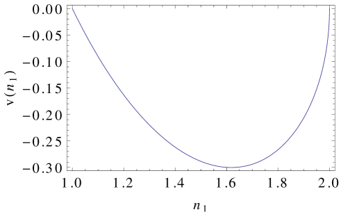
Figure 1: Effective potential for charge fluctuations in the two site case.

3.4.2 Time-dependent Gutzwiller approximation:

To solve the TDGA equations it is useful to note that $U_{2}=\infty$ leads to $D_{2}(t)\rightarrow 0$. If the constraints where exactly satisfied in the GA this would also imply $E_{1}(t)=0$. However, the numerical solution of the static GA shows that $E_{1}$ is nonzero but very small for any $U_{1}$ ($E_{1}<0.08$) and vanishes for $U_{1}\to-\infty$. In the following we assume for simplicity $E_{1}=0$. Then the constraint Eq. (42) implies $D_{1}=n_{1}-1$ and one can evaluate the TDGA equations analytically.

The hopping renormalisation factors simplify to,

$$q_{1\sigma} = e^{-\rmi(\chi_{1\sigma}+\eta_{1})}q_{d,1\sigma}\;,$$

$$q_{2\sigma} = e^{-\rmi\chi_{2\sigma}}q_{\emptyset,2\sigma}\;,$$

and the energy becomes

$$E^{GA}=-4t_{0}e^{-\rmi(\chi_{1\sigma}-\chi_{2\sigma}+\eta_{1})}\left(1-\frac{1}{n}_{1}\right)\rho_{21\sigma}+h.c.+U_{1}(n_{1}-1)\;.$$

The bonding single-particle state is defined by

$$\hat{h}_{1\sigma}^{\dagger}=u_{1\sigma}\hat{c}_{1\sigma}^{\dagger}+u_{2\sigma}\hat{c}_{2\sigma}^{\dagger}\;.$$

Without loss of generality we set $u_{1}=\sqrt{\frac{n_{1}}{2}}e^{\rmi\phi}$ and $u_{2}=\sqrt{\frac{n_{2}}{2}}$ which yields

$$\rho_{21\sigma}=e^{-\rmi\phi}\frac{\sqrt{n_{1}(2-n_{1})}}{2}\;,$$

and

$$\dot{u}_{1}u_{1}^{*}=\frac{\dot{n}_{1}}{4}+i\frac{n_{1}}{2}\dot{\phi}\;.$$

The Lagrangian reads,

$$L=-(U_{1}+\dot{\eta}_{1}+\dot{\phi})n_{1}-4t_{0}\cos(\eta_{1}+\phi)v(n_{1})\;,$$

where we chose a gauge in which $\chi=0$ and

$$v(n_{1})=-\left(1-\frac{1}{n}_{1}\right)\sqrt{n_{1}(2-n_{1})}\;.$$ (66)

Furthermore, since $\phi$ and $\eta_{1}$ play the same role, we can set $\phi=0$. Thus we get a Lagrangian with two dynamical variables $n_{1}$ and $\eta_{1}$ which are conjugate. Their equations of motion have the form,

$$\dot{n}_{1} = -4t_{0}\sin(\eta_{1})v(n_{1})\;,$$ (67)

$$\dot{\eta}_{1} = -U_{1}-4t_{0}\cos(\eta_{1})v^{\prime}(n_{1})\;.$$ (68)

The ‘potential’ $v(n_{1})$ is shown in Fig. 1. The static solution is given by $\eta_{1}=0$ and $v^{\prime}(n_{1})=-U_{1}/(4t_{0})$. Hence, for $U_{1}=0$ the static charge is $n_{1}^{0}=\frac{1}{2}\left(1+\sqrt{5}\right)\approx 1.62$ and it decreases towards $n_{1}=1$ when $U_{1}\rightarrow U_{1}^{c}=4t_{0}$ where a spurious Brinkman-Rice transition occurs. For negative $U_{1}$ instead the charge tends asymptotically to 2 when $U_{1}\rightarrow-\infty$.

Equations (67),(68) can be readily solved for small oscillations around the static solution. We find that the oscillatory frequency is $\omega_{0}=4t_{0}\sqrt{v^{\prime\prime}(n_{1}^{0})(-v(n_{1}^{0}))}$. For negative $U_{1}$ and until $U_{1}=0$ is approached we find that this frequency is in excellent agreement with the exact oscillation frequency of the two-site problem (c.f., Fig. 2). For positive $U_{1}$ as the spurious Brinkman-Rice point is approached, not surprisingly the approximations fail: the exact frequency increases monotonously as a function of $U_{1}$ while the approximate one vanishes at the Brinkman-Rice point. We attribute this to the failure of the GA in this finite-site system. Indeed we will show below that for high-dimensions a similar softening approaching a Mott state is real. The softening can be traced back to the fact that in the Brinkman-Rice phase the doublon charge gets frozen at zero therefore it is conserved and $\eta_{1}$ becomes a gauge phase which leads to an energy independent of $\eta_{1}$. We will see that a similar phenomena is found in the usual Brinkman-Rice transition.

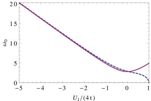
Figure 2: Oscillatory frequency in the TDGA for small amplitudes (dashed line) and in the exact solution for arbitrary fluctuations (full line) .

4 Linear response: The small amplitude limit

In the previous two-site model, the expansion of the effective potential $v(n_{1})$, Eq. (66), around the stationary value $n_{1}^{0}$ yields the dynamics in the vicinity of the GA saddle-point. Such an expansion is also important for the evaluation of response functions, where a (weak) external perturbation drives the system out of equilibrium.

Based on our general scheme derived in Sec. 2.4, the small amplitude limit is obtained by expanding the equations of motion, Eqs. (33),(36), around the ground state values $\tilde{\rho}^{0}$ and $\lambda^{0}_{\Gamma,\Gamma^{\prime}}$,

$$\tilde{\rho}(t) \approx \tilde{\rho}^{0}+\delta{{\rho}(t)}\;,$$ (69)

$$\lambda_{i;\Gamma,\Gamma^{\prime}}(t) \approx \lambda^{0}_{\Gamma,\Gamma^{\prime}}+\delta\lambda_{i;\Gamma,\Gamma^{\prime}}(t)\;.$$ (70)

For example, the first term on the r.h.s of Eq. (36) becomes

$$\frac{\partial E^{\rm GA}(\tilde{\lambda}^{(*)},\tilde{\rho})}{\partial\lambda_{i;\Gamma_{1},\Gamma_{2}}^{*}} \to \sum_{k,\Gamma_{3},\Gamma_{4}}\frac{\partial^{2}E^{\rm GA}(\tilde{\lambda}^{(*)},\tilde{\rho})}{\partial\lambda^{*}_{i;\Gamma_{1},\Gamma_{2}}\partial\lambda_{k;\Gamma_{3},\Gamma_{4}}}\delta\lambda_{k;\Gamma_{3},\Gamma_{4}}(t)$$ (71)

$$+ \sum_{\upsilon,\upsilon^{\prime}}\frac{\partial^{2}E^{\rm GA}(\tilde{\lambda}^{(*)},\tilde{\rho})}{\partial\lambda^{*}_{i;\Gamma_{1},\Gamma_{2}}\partial\rho_{\upsilon,\upsilon^{\prime}}}\delta\rho_{\upsilon,\upsilon^{\prime}}(t)\;.$$

After the linearisation of Eqs. (33) and (36) and with the harmonic Ansatz

$$\delta\lambda_{i;\Gamma,\Gamma^{\prime}}(t) = \delta\lambda_{i;\Gamma,\Gamma^{\prime}}(\omega)e^{\rmi\omega t}\;,$$ (72)

$$\delta\rho_{\upsilon,\upsilon^{\prime}}(t) = \delta\rho_{\upsilon,\upsilon^{\prime}}(\omega)e^{\rmi\omega t}\;,$$ (73)

we finally end up with a linear set of equations for $\lambda_{i;\Gamma,\Gamma^{\prime}}(\omega)$ and $\delta\rho_{\upsilon,\upsilon^{\prime}}(\omega)$ which can be solved numerically.  Note that at zero frequency, the l.h.s. of Eq. (36) vanishes.  This equation then recovers exactly the ‘antiadiabaticity assumption’ which was used in the previous TDGA formulation [5, 6, 7, 8].  Within the single band Hubbard model we will demonstrate in the following that the inclusion of the full time-dependence of the variational parameters $\lambda_{i;\Gamma,\Gamma^{\prime}}(t)$ generates additional features in the dynamical charge correlations which are absent in the ‘antiadiabatic approximation’.

5 Response functions in the single-band Hubbard model

In the single-band Hubbard model the three most relevant response channels are related to the coupling to time-dependent magnetic, charge and pair fields. This requires the computation of the (transversal) ‘magnetic susceptibility’

$$\chi^{\rm T}_{i,j}(t)=\langle\langle\hat{c}^{\dagger}_{i,\uparrow}\hat{c}^{\phantom{\dagger}}_{i,\downarrow};\hat{c}^{\dagger}_{j,\downarrow}\hat{c}^{\phantom{\dagger}}_{j,\uparrow}\rangle\rangle(t)\;,$$ (74)

the ‘charge susceptibility’

$$\chi^{\rm C}_{i,j}(t)=\langle\langle\hat{n}_{i};\hat{n}_{j}\rangle\rangle(t)\;,$$ (75)

and the ‘pairing susceptibility’

$$\chi^{\rm P}_{i,j}(t)=\langle\langle\hat{c}^{\dagger}_{i,\uparrow}\hat{c}^{\dagger}_{i,\downarrow};\hat{c}^{\phantom{\dagger}}_{j,\downarrow}\hat{c}^{\phantom{\dagger}}_{j,\uparrow}\rangle\rangle(t)\;,$$ (76)

or their respective Fourier transforms

$$\chi^{\rm T/C/P}(\vec{q},\omega)=\frac{1}{L}\int_{-\infty}^{\infty}e^{\rmi\omega t}\sum_{i,j}e^{\rmi(\vec{R}_{i}-\vec{R}_{j})\vec{q}}\chi^{\rm T/C/P}_{i,j}(t)\;,$$ (77)

where we have introduced $\hat{n}_{i}=\sum_{\sigma}\hat{n}_{i,\sigma}$.

5.1 The magnetic and the pairing susceptibility

If the state $|\Psi_{\rm S}\rangle$ is paramagnetic or is restricted to longitudinal magnetic order, the charge and (transverse) magnetic susceptibilities are decoupled.  Moreover, if the ground state does not contain superconducting correlations, also the pairing fluctuations are decoupled from the magnetic and charge correlations. In this case, the (mixed) second derivative of the energy with respect to $\langle\hat{c}^{\dagger}_{i,\uparrow}\hat{c}^{\phantom{\dagger}}_{i,\downarrow}\rangle$ and $\lambda_{i;d}$ vanishes. In a similar way, one can show that the second derivative with respect to pairing fluctuations $\langle\hat{c}^{\dagger}_{i,\uparrow}\hat{c}^{\dagger}_{i,\downarrow}\rangle$ and $\delta\lambda_{i;d}$ vanishes. Therefore, in both cases, the linearised differential equations (33) and (36) are decoupled and the time dependence of $\delta\lambda_{i;d}(t)$ does not enter the computation of (transverse) magnetic and pairing correlation functions. The susceptibilities are then solely determined by the solution of Eq. (33) for the single-particle density matrix and the present approach agrees with the previous formulation of the TDGA involving the ‘antiadiabaticity approximation’ [5, 6, 7, 8]. Therefore we concentrate in the following on the investigation of the dynamical charge-charge correlation function where the present approach is able to capture high-energy excitations on the scale of the Hubbard repulsion due to the explicit time dependence of the variational parameters.

5.2 Dynamical charge susceptibility

As derived in Sec. 3, the time dependence of the system is governed by small deviations of the density matrix $\delta\tilde{\rho}$, the double-occupancy parameters $\delta D_{i}$ and the phase $\delta\eta_{i}$ from their saddle-point values (indicated by a ‘$0$’ superscript). Note that we consider a GA ground state with $\eta_{i}^{0}=0$ such that $\delta\eta_{i}=\eta_{i}$. The corresponding equations of motion

$$-\dot{\eta}_{i} = \frac{\partial E^{\rm GA}}{\partial\delta D_{i}}\;,$$ (78)

$$\dot{\delta D}_{i} = \frac{\partial E^{\rm GA}}{\partial\eta_{i}}\;,$$ (79)

$$\rmi\delta\dot{\tilde{\rho}} = [\tilde{h}^{\rm GA},\delta\tilde{\rho}]\;,$$ (80)

have to be solved for small deviations from the GA saddle-point. For this purpose we expand the Gutzwiller energy functional Eq. (54) up to second order in the fluctuations

$$E^{\rm GA}=E^{\rm GA,0}+E^{\rm GA,1}+E^{\rm GA,2}$$ (81)

around the saddle-point value $E^{\rm GA,0}$.

The first order contribution yields

$$E^{\rm GA,1} = Tr\{\tilde{h}^{\rm GA}\delta\tilde{\rho}\}+\sum_{i}\left(\frac{\partial E^{\rm GA}}{\partial D_{i}}\delta D_{i}+\frac{\partial E^{\rm GA}}{\partial\eta_{i}}\eta_{i}\right)$$ (82)

and the derivatives have to be taken at the saddle-point. Here, the first term describes particle-hole excitations within the ‘bare’ Gutzwiller Hamiltonian. The second term $\sim\delta D_{i}$ vanishes due to the saddle-point condition, whereas the last term can be expressed in the small amplitude limit as

$$\frac{\partial E^{\rm GA}}{\partial\eta_{i}}=\rmi\sum_{\sigma}\frac{q^{0}_{d,i,\sigma}}{q^{0}_{\emptyset,i,\sigma}+q^{0}_{d,i,\sigma}}\left[\delta\rho_{i\sigma},\tilde{h}^{\rm GA}\right]=\sum_{\sigma}\frac{q^{0}_{d,i,\sigma}}{q^{0}_{\emptyset,i,\sigma}+q^{0}_{d,i,\sigma}}\delta\dot{\rho}_{i\sigma}\;,$$ (83)

where we have made use of Eq. (80). Thus in the small amplitude limit it is convenient to introduce a ’displaced double occupancy’

$$\tilde{D}_{i}=D_{i}-\sum_{\sigma}\frac{q^{0}_{d,i,\sigma}}{q^{0}_{\emptyset,i,\sigma}+q^{0}_{d,i,\sigma}}\delta{\rho}_{i\sigma}$$ (84)

such that the dynamics of $\eta_{i}$ and $\delta\tilde{D}_{i}$ can be expressed via the second order contribution of $E^{\rm GA}$ as

$$-\dot{\eta}_{i} = \frac{\partial E^{\rm GA,2}}{\partial\delta\tilde{D}_{i}}\;,$$ (85)

$$\delta\dot{\tilde{D}}_{i} = \frac{\partial E^{\rm GA,2}}{\partial\eta_{i}}\,.$$ (86)

The following evaluation of $E^{\rm GA,2}$ is exemplified for a homogeneous paramagnet but can be straightforwardly generalised to arbitrary ground states. In momentum space the second order expansion involves fluctuations of $\eta_{q}$ and $\delta\tilde{D}_{q}$ which are coupled to fluctuations of the local $\delta\rho_{q}=\sum_{k,\sigma}\delta\rho_{k+q,k}^{\sigma}$ and transitive $\delta T^{+}_{q}=\sum_{k,\sigma}\left[\varepsilon^{0}_{k+q}+\varepsilon^{0}_{k}\right]\delta\rho_{k+q,k}^{\sigma}$ charge densities:

$$\delta E^{\rm GA,2} = \frac{1}{2N}\sum V_{q}\delta\rho_{q}\delta\rho_{-q}+V^{T\rho}\frac{1}{N}\sum_{q}\delta T^{+}_{q}\delta\rho_{-q}$$ (87)

$$+ \frac{1}{\sqrt{N}}\sum_{q}g^{\tilde{D}\rho}_{q}\delta\tilde{D}_{-q}\delta\rho_{q}+\frac{1}{\sqrt{N}}\sum_{q}g^{\tilde{D}T}_{q}\delta\tilde{D}_{-q}\delta T^{+}_{q}$$

$$+ \frac{1}{2}\sum_{q}K_{q}\delta\tilde{D}_{q}\delta\tilde{D}_{-q}+\frac{1}{2}\sum_{q}\frac{1}{M}\eta_{q}\eta_{-q}$$

with

$$V_{q} = \frac{1}{2}e_{0}q^{0}(z_{++}^{\prime\prime}+2z_{+-}^{\prime\prime}+z_{--}^{\prime\prime})+\frac{1}{2}(z^{\prime}+z_{+-}^{\prime})^{2}\frac{1}{N}\sum_{k,\sigma}\varepsilon^{0}_{k+q}\langle n_{k,\sigma}\rangle$$ (88)

$$+ 2\frac{q^{0}_{d}}{q^{0}_{\emptyset}+q^{0}_{d}}\left(L_{q}+\frac{K_{q}}{2}\frac{q^{0}_{d}}{q^{0}_{\emptyset}+q^{0}_{d}}\right)\;,$$

$$V^{T\rho} = \frac{1}{2}q^{0}(z^{\prime}+z^{\prime}_{+-})+q^{0}z_{D}^{\prime}\frac{q^{0}_{d}}{q^{0}_{\emptyset}+q^{0}_{d}}\;,$$ (89)

$$g^{\tilde{D}\rho}_{q} = L_{q}+K_{q}\frac{q^{0}_{d}}{q^{0}_{\emptyset}+q^{0}_{d}}\;,$$ (90)

$$g^{\tilde{D}T}_{q} = q^{0}z_{D}^{\prime}\;,$$ (91)

$$K_{q} = 2(z_{D}^{\prime})^{2}\frac{1}{N}\sum_{k,\sigma}\varepsilon^{0}_{k+q}\langle n_{k,\sigma}\rangle+2\varepsilon^{0}q^{0}z_{D}^{\prime\prime}\;,$$ (92)

$$\frac{1}{M} = -2\varepsilon^{0}q^{0}_{\emptyset}q^{0}_{d}\;,$$ (93)

$$L_{q} = e_{0}q^{0}(z_{+D}^{\prime\prime}+z_{-D}^{\prime\prime})+z_{D}^{\prime}(z^{\prime}+z_{+-}^{\prime})\frac{1}{N}\sum_{k,\sigma}\varepsilon^{0}_{k+q}\langle n_{k,\sigma}\rangle$$ (94)

where at the saddle point the renormalisation factors become site and spin independent (i.e. $q^{0}_{\emptyset,i,\sigma}=q^{0}_{\emptyset}$, $q^{0}_{d,i,\sigma}=q^{0}_{d}$, $q^{0}_{i\sigma}=q^{0}$) and the primed letters denote derivatives which are specified in B. We have also defined the non-renormalised single-particle dispersion $\varepsilon^{0}_{k}$, whereas the GA quasi-particle dispersion will be denoted as $\varepsilon_{k}=(q_{i,\sigma})^{2}\varepsilon^{0}_{k}$. Then from Eqs. (85),(86) the phase and double-occupancy dynamics is given by

$$-\dot{\eta}_{q} = \frac{\partial E^{\rm GA,2}}{\partial\delta\tilde{D}_{-q}}$$ (95)

$$= \frac{1}{\sqrt{N}}g^{\tilde{D}\rho}_{q}\delta\rho_{q}+\frac{1}{\sqrt{N}}g^{\tilde{D}T}_{q}\delta T^{+}_{q}+K_{q}\delta{\tilde{D}}_{q}\;,$$

$$\delta\dot{\tilde{D}}_{q} = \frac{\partial E^{\rm GA,2}}{\partial\eta_{-q}}=\frac{1}{M}\eta_{q}\;,$$ (96)

which upon Fourier transforming in the time domain yields for the double occupancy

$$\tilde{D}_{q}=\frac{1}{\sqrt{N}}\left(\gamma^{\tilde{D}\rho}_{q}\delta\rho_{q}+\gamma^{\tilde{D}T}_{q}\delta T^{+}_{q}\right){\cal D}^{0}(q,\omega)\;.$$ (97)

Here we have defined the renormalised couplings

$$\gamma^{\tilde{D}\rho}_{q} = \frac{g^{\tilde{D}\rho}_{q}}{\sqrt{2\Omega_{q}M}}\;,$$ (98)

$$\gamma^{\tilde{D}T}_{q} = \frac{g^{\tilde{D}T}_{q}}{\sqrt{2\Omega_{q}M}}\;,$$ (99)

and the ‘double occupancy’ Green’s function

$${\cal D}^{0}(q,\omega)=\frac{2\Omega_{q}}{\omega^{2}-\Omega_{q}^{2}}\;,$$ (100)

which has poles at $\Omega_{q}^{2}=K_{q}/M$. In case of a half-filled system one obtains

$$\Omega_{q}^{2}=16\varepsilon_{0}^{2}\left[1-u^{2}\kappa_{q}\right]\;,$$ (101)

where $\varepsilon_{0}$ is the energy of the non-interacting system, $u\equiv U/|8\varepsilon_{0}|$, and $\kappa_{q}=\frac{1}{\cal D}\sum_{i=1}^{\cal D}\cos(q_{i})$ . Interestingly the Brinkman-Rice transition $u=1$ can therefore be associated with a ‘soft mode’ where $\Omega_{q=0}\to 0$. This softening is clearly associated to the extra gauge invariance condition that appears at the Brinkman-Rice point which makes the mass $M$ to diverge.

Equations (87)-(96) show that in the present approach the interacting electron problem can be mapped to an effective electron-boson problem. Electron quasiparticles are coupled to a boson representing fluctuations of the double occupancy (“doublon fluctuations”) or of its conjugate variable. Notice that the mass $M$ of the fluctuation field diverges in the two situations discussed after Eq. (55) either $E\rightarrow 0$ of $D\rightarrow 0$ (c.f Eqs. (49),(61) and (93). This follows from the fact that in those cases $\eta$ becomes a gauge phase and therefore gauge invariance requires that the last term of Eq. (87) vanishes.

In analogy with electron-phonon problems the dressed fluctuations are most conveniently evaluated by defining a (non-interacting) susceptibility matrix

$$\underline{\underline{\chi^{ee,0}_{q}(\omega)}} = \frac{-1}{N}\int_{0}^{\beta}d\tau\mbox{e}^{i\omega_{n}\tau}\left(\begin{array}[]{cc}\langle{\cal T}\delta\rho_{\bf q}(\tau)\delta\rho_{-{\bf q}}(0)\rangle&\langle{\cal T}\delta\rho_{\bf q}(\tau)\delta T^{+}_{-{\bf q}}(0)\rangle\\ \langle{\cal T}\delta T^{+}_{\bf q}(\tau)\delta\rho_{-{\bf q}}(0)\rangle&\langle{\cal T}\delta T^{+}_{\bf q}(\tau)\delta T^{+}_{-{\bf q}}(0)\rangle\\ \end{array}\right)$$ (104)

$$= \frac{1}{N}\sum_{k\sigma}\left(\begin{array}[]{ccc}1&\epsilon^{0}_{{\bf k}+{\bf q}}+\epsilon^{0}_{\bf k}\\ \epsilon^{0}_{{\bf k}+{\bf q}}+\epsilon^{0}_{\bf k}&\left(\epsilon^{0}_{{\bf k}+{\bf q}}+\epsilon^{0}_{\bf k}\right)^{2}\\ \end{array}\right)\frac{n_{k+q,\sigma}-n_{k\sigma}}{\omega+\epsilon_{k+q}-\epsilon_{k}}$$ (107)

and an effective interaction matrix which is composed of the bare electron-electron interaction and the second order ‘bosonic contribution’

$$\underline{\underline{\widetilde{V}^{ee}_{q}(\omega_{n})}}=\left(\begin{array}[]{cc}V_{q}&V^{T\rho}\\ V^{T\rho}&0\end{array}\right)+\left(\begin{array}[]{cc}(\gamma^{\tilde{D}\rho}_{q})^{2}&\gamma^{\tilde{D}\rho}_{q}g^{AT}_{q}\\ \gamma^{\tilde{D}\rho}_{q}\gamma^{\tilde{D}T}_{q}&(\gamma^{AT}_{q})^{2}\end{array}\right){\cal D}^{0}(q,\omega)\,.$$

The susceptibility for the interacting system is then obtained from the following RPA series

$$\underline{\underline{\chi_{q}}}=\underline{\underline{\chi^{0}_{q}}}+\underline{\underline{\chi^{0}_{q}}}\,\underline{\underline{\widetilde{V}^{ee}_{q}}}\underline{\underline{\chi_{q}}}$$ (108)

Note that in the static limit $\omega\to 0$ the matrix $\underline{\underline{\widetilde{V}^{ee}_{q}(0)}}$ is exactly the effective interaction obtained within the antiadiabaticity condition in Refs. [5, 6].

6 Results

In this section, we present results for the local dynamical charge correlation function

$$\chi_{\rm loc}(\omega)=\sum_{q\neq 0}\frac{|\langle 0|\hat{n}_{i}|q\rangle|^{2}}{\omega+E_{q}-E_{0}-\rmi\eta}$$ (109)

where $|0\rangle$ and $|q\rangle$ denote ground and excited states of the single-band Hubbard model. We first study the low-density regime where we compare the TDGA spectra with exact results for the case of two particles. For higher densities we study the performance of the TDGA by comparing with DMFT and exact diagonalisation results.

6.1 Low-density regime

In the low-density limit $n\to 0$ the energy of the non-interacting system is determined by $\varepsilon_{0}=-Bn$ where $2B$ would be the total bandwidth in case of a rectangular density of states. The saddle point double occupancy in this limit reads as

$$D_{n\to 0}^{0}=\frac{n^{2}}{4}\frac{1}{\left(1+\frac{U}{2B}\right)^{2}}$$ (110)

which allows for the computation of the frequency of double-occupancy oscillations as $\Omega_{q}=2B+U$, i.e., it is independent of momentum. Since the coupling to these fluctuations Eqs. (98),(99) vanishes with $n$ we expect the local TDGA charge correlations to be composed of a renormalised low-energy part for $0<\omega<2B$ and a high-energy excitation at $\omega=2B+U$ with spectral weight proportional to the density.

In case of two particles one can determine the eigenenergies in Eq. (109) from [32]

$$\frac{1}{U}=\frac{1}{N}\sum_{k}\frac{1}{E-\epsilon_{k}-\epsilon_{k+q}}$$ (111)

where $-4t\leq\epsilon_{k}\leq 4t$ denotes the single-particle dispersion with bandwidth $2B=8t$. The ground state is obtained for $q=0$ and both particles at the bottom of the band, i.e., $E_{0}\approx-2B$. A particular solution in Eq. (111) is obtained for ${\bf Q}={\bf q}=(\pi,\pi)$ at $E_{\bf Q}=U$ so that the excited state $E_{\bf Q}-E_{0}=2B+U$ corresponds to our TDGA result discussed above.  In addition, the exact solution involves two-particle excitations which are not present in the TDGA. The maximum excitation energy is obtained for $q=0$ which can be estimated for a rectangular density of states as $\omega=4B/(e^{1/U}-1)$. The weight of these excitations in Eq. (111) vanishes for zero momentum transfer but clearly the exact solution displays high energy features in addition to the TDGA for small ${\bf q}$ due to the coupling between particle-hole and particle-particle excitations.

Figure 3 displays the low-density local charge susceptibility Eq. (111), evaluated with TDGA and exact diagonalisation for $U/t=5$ and $U/t=10$, respectively. Results have been obtained for $2$ particles on a $8\times 8$ square lattice lattice (only nearest neighbor hopping $-t$).

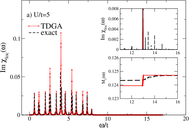
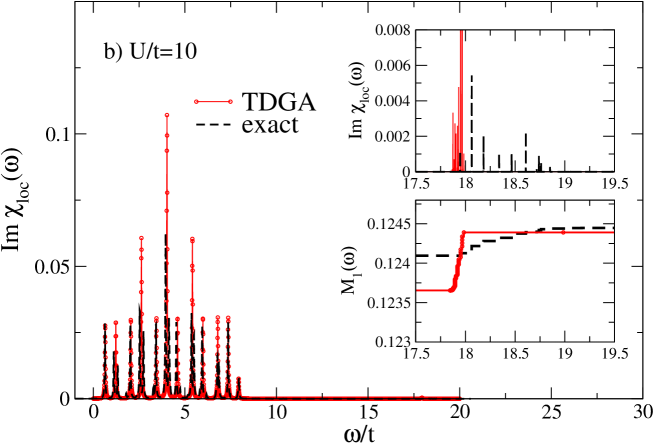
Figure 3: Local charge susceptibility for $2$ particles on a $8\times 8$ lattice with (a) $U/t=5$ and (b) $U/t=10$. We compare spectra for the exact result (black, dashed) with those obtained within the TDGA (solid, circles). The upper insets show the high-energy part of the spectra. Broadening of the excitations is $\epsilon=0.02t$ (main panels) and $\epsilon=10^{-4}t$ (upper insets). The lower insets depict the high-energy part of the first moments $M_{1}(\omega)$.

As anticipated above, the spectra consist of the (dominant) low-energy bandlike particle-hole excitations in the range $0<\omega<2B$ (cf. main panels) and a high-energy part at $\omega\approx 2B+U$ which is resolved in the upper insets. Similar to the previous investigations, which were based on the ‘antiadiabaticity assumption’ [5, 6], the TDGA gives a very good account of the low-energy part with respect to both, energy and spectral weight of the excitations. The new feature, which was previously missing [5, 6] in the TDGA, is the high-energy part due to the explicit consideration of the double-occupancy time dependence. In order to estimate the associated spectral weight, we show in the lower insets to Fig. 3 the first moment

$$M_{1}(\omega)=\int_{0}^{\omega}\!\!d\nu\,\nu\,\chi_{\rm loc}(\nu)\;,$$ (112)

which fulfills the sum rule

$$M_{1}(\infty)=-\langle T\rangle\;.$$ (113)

Here $\langle T\rangle$ denotes the kinetic energy which in case of the TDGA has to be evaluated on the basis of the GA. From Fig. 3 it turns out that the onset of the high-energy excitations is accurately captured by the TDGA, however, it overestimates the associated spectral weight. On the other hand, this ‘additional’ weight is partially compensated for in the bandlike excitations such that the kinetic energy of the Gutzwiller approximation (i.e. $M_{1}(\infty)$) again gives a good account of the exact result.

6.2 Density dependence

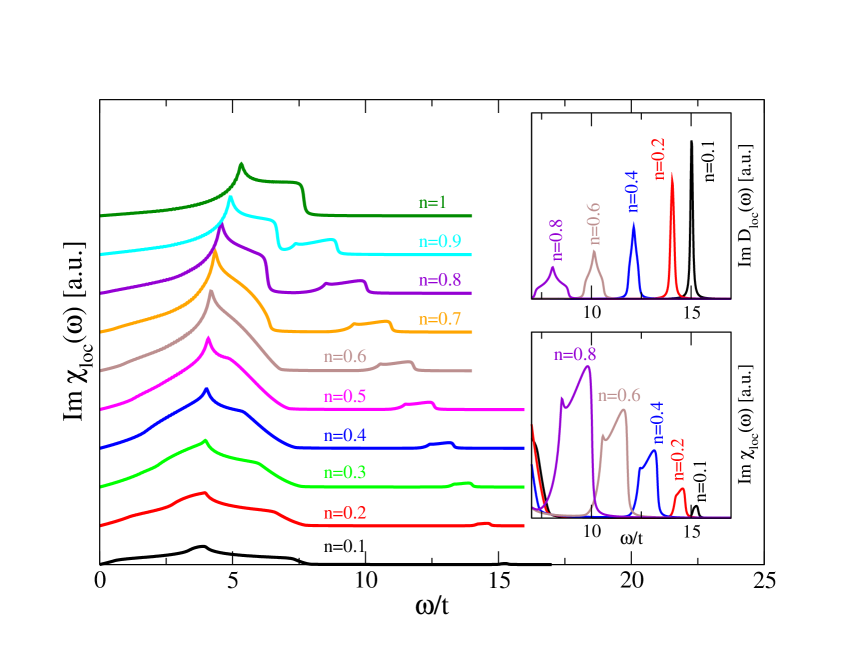
Figure 4: TDGA local charge susceptibility for a two-dimensional square lattice Hubbard model ($U/t=8$, nearest-neighbor hopping $-t$) at different densities. The inset displays the high-energy part on an enlarged scale whereas the upper inset shows the imaginary part of the double-occupancy propagator.

We proceed by studying the doping dependence of $\chi_{\rm loc}(\omega)$ as a function of doping which is shown in Fig. 4 for $U/t=8$ for a square lattice. The spectra again separate into low-energy band-like excitations and a high-energy part due to the double-occupancy time dependence. Starting form the low density limit the overall weight of the high-energy excitations increases approaching half filling. In addition the high-energy feature shifts to lower frequencies upon doping as shown in the lower inset to Fig. (4).

We show also in the upper inset the imaginary part of the local double-occupancy propagator, i.e.

$${\mbox{Im}}D_{\rm loc}^{0}(\omega)={\mbox{Im}}\frac{1}{N}\sum_{q}{\cal D}^{0}(q,\omega)$$ (114)

and ${\cal D}(q,\omega)$ has been defined in Eq. (100).

The double-occupancy excitations evolve from $\Omega=2B+U$ ($=16t$ for the present parameters) in the limit $n\to 0$ to the frequencies $\Omega_{q}$ defined in Eq. (101) for the case of half-filling. In order to understand the doping dependence of the high-energy feature one has also to take into account the couplings Eqs. (98),(99). The coupling to the local fluctuations, $\gamma_{q}^{\tilde{D}\rho}$ [Eq. (98)] is continuously decreasing with the charge carrier concentration and dominates at all dopings except close to half-filling where it vanishes. On the other hand, the coupling to transitive fluctuations $\gamma_{q}^{\tilde{D}T}$ [Eq. (99)] is significantly smaller and only weakly doping dependent. Since at half-filling the coupling between local and transitive fluctuations vanishes ($V^{T\rho}=0$), the local charge correlations are only renormalised by the static density-density interactions $V_{q}$. Thus at exactly half-filling the coupling to the double-occupancy fluctuations vanishes and the $n=1$ curve in Fig. (4) corresponds to the ‘antiadiabaticity’ result derived in Refs. [5, 6]. With decreasing doping the increasing coupling between local density and double fluctuations increases and induces the shift of the high-energy feature to large frequencies.

In order to check the quality of the TDGA at larger doping vs. other approaches we compare our results with dynamical mean-field theory (DMFT)[33]. Despite freezing the spatial fluctuations beyond mean-field, DMFT takes fully into account the local quantum dynamics and it is in particular reliable to describe the evolution of the spectral weight as a function of temperature and other control parameters like doping. DMFT maps the lattice model onto an Anderson Impurity model, which is solved with an ‘impurity solver’, which in the present work is exact diagonalisation [34]. Within this method the bath of the AIM is discretised into $N_{b}$ levels, which here is taken to be 9. A Matsubara grid defined by an effective temperature $\beta=80/t$ is used and the stability of the results as a function of the two control parameters has been checked. Within DMFT, the local dynamical correlation functions can be obtained without further approximation. As a result of the discrete bath, the spectra appear more spiky than in the actual solution, but it has been shown that this approach describes accurately the evolution of the spectral weight (for instance of the optical conductivity) as a function of the various control parameters [35, 36].

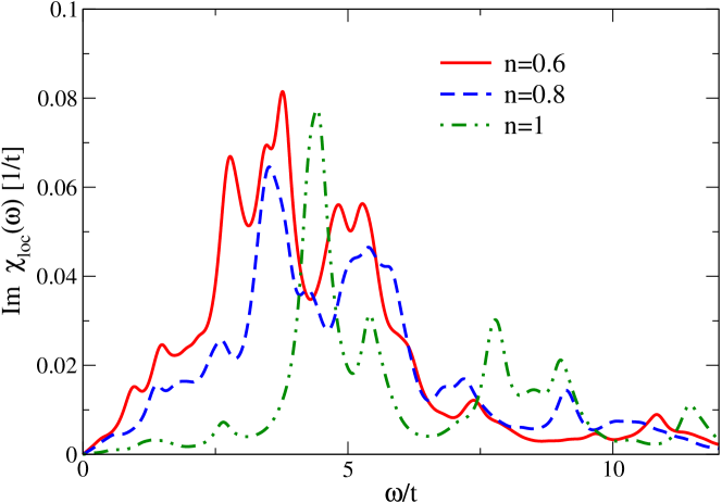
Figure 5: DMFT local charge susceptibility for a two-dimensional square lattice Hubbard model ($U/t=8$, nearest-neighbor hopping $-t$) at densities $n=0.6$, $n=0.8$, and $n=1$.

Figure 5 (main panel) shows the local charge susceptibility obtained within DMFT for different fillings and $U/t=8$. Despite the peaky structure (which hampers a direct comparison with the TDGA results) it is obvious that the main features correspond to those obtained within the TDGA, i.e., bandlike excitations on the scale of $8t$ and additional higher energy excitations which soften and gain spectral weight upon increasing density and approaching the insulating phase.

In order to test the performance of the TDGA we show in Fig. 6 (panels b,d) a comparison of the first moment $M_{1}(\omega)$, Eq. (112), evaluated within TDGA (black solid lines) and DMFT (green circles) for $U/t=8$ and densities $n=0.6$ (panel b) and $n=1.0$ (panel d). As anticipated above the TDGA gives a rather good account of the spectral weight evolution at lower densities where it is in good agreement with the DMFT data (Fig. 6, panel b) given the uncertainties due to the finite number of bath states. However, due to the vanishing coupling between electrons and double-occupancy fluctuations at half-filling, all the TDGA spectral weight is contained in the band-like excitations in this limit so that the ‘antiadiabaticity’ result of Refs. [5, 6] is recovered. Therefore the corresponding first moment increases much faster than DMFT but nevertheless both moments approach for $\omega\to\infty$ due to the agreement in the kinetic energies. One should note that at half-filling the GA ground state actually corresponds to a spin-density wave and also for such symmetry-broken states we find that at half-filling the antiadiabaticity result of Refs. [5, 6] is valid. In fact, the TDGA charge excitations on top of such a ground state are in reasonable agreement with exact diagonalisation as demonstrated in Fig. 5 of Ref. [6].

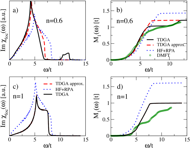
Figure 6: Imaginary part of the local charge susceptibility at densities $n=0.6$ (panel a) and $n=1$ (panel c) evaluated with the TDGA (solid black), TDGA with antiadiabaticity (dashed red), and HF+RPA (dotted blue). Panels c,d report the corresponding evolution of the first moment Eq. (112) where also the results from DMFT (circles, green) are shown. Onsite repulsion: $U/t=8$.

For comparison, we also show in Fig. 6 the result of HF+RPA theory together with the spectra of our previous ‘approximate’ TDGA [5, 6] where the double-occupancy fluctuations have been antiadiabatically eliminated. As discussed above, at half-filling the antiadiabatic approximation agrees with the ‘exact’ evaluation of the TDGA (cf. panels c,d in Fig. 6). The difference becomes pronounced at lower doping where the high-energy feature gets significant spectral weight and due to repulsion induces a softening of the bandlike excitations. From panel a of Fig. 6 it is clear that both effects are essential for reproducing the very good agreement of the first moment with the DMFT result at $n=0.6$ whereas the approximate TDGA interpolates the spectral weight between the bandlike and high-energy excitations. Note, however, that for small frequencies $\omega\to 0$ the approximate result agrees with the ‘exact’ TDGA as has already been discussed in Sec. 4. In addition, the first moment of both approaches agrees in the limit $\omega\to\infty$ since it is set by the static GA kinetic energy.

In case of the conventional HF+RPA approach, where the local charge susceptibility is given by

$$\chi_{\rm loc}^{\rm HF+RPA}(\omega)=\frac{1}{N}\sum_{q}\frac{\chi^{0}_{q}(\omega)}{1-\frac{U}{2}\chi^{0}_{q}(\omega)}$$ (115)

and $\chi^{0}_{q}(\omega)$ has the same structure than the $(11)$-element of Eq. (107) but with non-renormalised single-particle dispersions $\varepsilon_{k}^{0}$. Since HF+RPA obviously does not capture the double-occupancy dynamics, the local charge fluctuations originate from the band-type excitations which are renormalised due to the RPA denominator and high frequency excitations are absent. Moreover, HF overestimates the kinetic energy so that the first moment of $\chi_{\rm loc}^{\rm HF+RPA}$ overshoots both the TDGA and DMFT result. As can be seen from Fig. 6 this discrepancy is most apparent close to half-filling where the renormalisation of the kinetic energy due to correlation effects is more pronounced. Upon reducing the band filling the low-energy part of the HF+RPA spectra approaches the TDGA result where, however, the latter approach additionally captures the high frequency excitations at $2B+U$ with spectral weight $\sim n$.

7 Conclusions

In this paper we have developed the time-dependent Gutzwiller approximation for multi-band Hubbard models. This approach is based on a time-dependent variational principle where expectation values are evaluated with the Gutzwiller variational wave-function in the limit of infinite dimensions. In contrast to the standard Gutzwiller approximation [9, 10, 11] both, variational parameters and the underlying Slater determinant, acquire a time dependence. In this regard our calculations generalise earlier investigations by Schiró and Fabrizio [21, 22] who have studied quantum quenches in homogeneous systems where the time dependence of the density matrix does not couple to that of the variational parameters. On the other hand, momentum (or space) dependent out-of equilibrium displacements of the system require such a coupling as evident from our generalised equations of motion Eqs. (33),(36).

We have applied this theory in the small-amplitude, i.e., linear-response limit and exemplified for the case of dynamical charge correlations in the single-band Hubbard model. In an earlier formulation of the TDGA the so-called ‘antiadiabaticity approximation’ [5, 6] has been applied, where the dynamics of the double-occupancy parameters was slaved by that of the density matrix.  In contrast, the present approach explicitly incorporates the time dependence of the double-occupancy variational parameters which agrees with the previous formulation in the static limit. In addition it improves the theory in Refs. [5, 6] by incorporating the high-energy features which are on the scale of the Hubbard repulsion for small densities and which position is in good agreement with that of exact diagonalisation. On the other hand, the spectral weight of the high-energy excitations is overestimated within the TDGA although it significantly improves the standard HF+RPA approach in this regard. Further refinement of the theory could be achieved by including the coupling between particle-hole and particle-particle excitations which have been studied in Ref. [8] in the framework of the GA.

It is interesting that in the present approach the Brinkman-Rice transition appears signaled by a collective mode whose frequency goes to zero. This is not due to the doublon fluctuation stiffness becoming soft but because the mass of the fluctuations diverges. We have shown that this divergence appears each time the double occupancy becomes a conserved quantity which is the case in the Brinkman-Rice case where $D=0$. It remains to be seen which of these feature remain in an exact description although the similarity of the TDGA results with dynamical mean field theory (DMFT) suggest that at least in an approximate way this physics survives in real Mott transitions.

Within the DMFT it is quite diffult to study systems in which the momentum dependence of collective excitations is important as, for example, spin waves in insulators [37]. In such cases, the TDGA provides us with an important additional tool which complements the DMFT.

8 Acknowledgments

M. C. is financed by EU/FP7 through ERC Starting Grant SUPERBAD, Grant Agreement 240524, and GO FAST, Grant Agreement 280555. J. L. is supported by the Italian Institute of Technology through the project NEWDFESCM.

Appendix A Physical meaning of the phases

To understand the physical meaning of the phases appearing in Eq. (48) and how they affect the hopping amplitude consider the following two-site example in which the non interacting state is uniform,

$$|\Psi_{\rm S}\rangle=\frac{1}{2}(\hat{c}_{1,\uparrow}^{\dagger}+\hat{c}_{2,\uparrow}^{\dagger})(\hat{c}_{1,\downarrow}^{\dagger}+\hat{c}_{2,\downarrow}^{\dagger})|{\rm vac}\rangle$$

but the projectors are given by Eq. (40) with all $\lambda_{\Gamma}=1$ except $\lambda_{2d}=-1$ which corresponds to $\eta_{2}=\pi$ and the other phases zero leading to $q_{2,\sigma}=0$, i.e., destructive interference. The projected wave function reads,

$$|\Psi_{G}\rangle=\frac{1}{2}(\hat{c}_{1,\uparrow}^{\dagger}\hat{c}_{1,\downarrow}^{\dagger}-\hat{c}_{2,\uparrow}^{\dagger}\hat{c}_{2,\downarrow}^{\dagger}+\hat{c}_{1,\uparrow}^{\dagger}\hat{c}_{2,\downarrow}^{\dagger}+\hat{c}_{2,\uparrow}^{\dagger}\hat{c}_{1,\downarrow}^{\dagger})|{\rm vac}\rangle\;.$$

The exact off-diagonal density matrix in the Gutzwiller wave function is given by the overlap between the states,

$$\hat{c}_{1,\uparrow}|\Psi_{G}\rangle = \frac{1}{2}(\hat{c}_{1,\uparrow}^{\dagger}+\hat{c}_{2,\uparrow}^{\dagger})|{\rm vac}\rangle\;,$$

$$\hat{c}_{2,\uparrow}|\Psi_{G}\rangle = \frac{1}{2}(\hat{c}_{1,\uparrow}^{\dagger}-\hat{c}_{2,\uparrow}^{\dagger})|{\rm vac}\rangle\;.$$

We see that in this zero dimensional example the ‘background’ electron remains with the ‘wrong’ phase (or momentum) leading to zero overlap, in accord with the GA derived in infinite dimensions. Notice, however, that if also $\lambda_{1d}=-1$ the overlap is finite in the exact evaluation while it is zero in the GA. Clearly such kind of process depends on the correlation between the phases on different sites and can not be captured by the factorised form $\sim q_{1,\sigma}^{*}q_{2,\sigma}$ of the GA.

Appendix B Derivatives of the renormalisation factors

In Sec. 5.2 we have introduced derivatives of the hopping renormalisation factor $q_{i,\sigma}$, evaluated at the saddle-point of a paramagnetic system. These are defined as follows:

$$\frac{\partial q_{i\sigma}}{\partial\rho_{ii\sigma}}\equiv z^{{}^{\prime}},\ \ \ \frac{\partial q_{i\sigma}}{\partial\rho_{ii-\sigma}}\equiv z^{{}^{\prime}}_{+-},\ \frac{\partial q_{i\sigma}}{\partial D_{i}}\equiv z^{{}^{\prime}}_{D}$$

$$\frac{\partial^{2}q_{i\sigma}}{\partial\rho^{2}_{ii\sigma}}\equiv z^{{}^{\prime\prime}}_{++},\ \frac{\partial^{2}q_{i\sigma}}{\partial\rho_{ii\sigma}\partial\rho_{ii-\sigma}}\equiv z^{{}^{\prime\prime}}_{+-},\ \frac{\partial^{2}q_{i\sigma}}{\partial\rho^{2}_{ii-\sigma}}\equiv z^{{}^{\prime\prime}}_{--}$$

$$\frac{\partial^{2}q_{i\sigma}}{\partial D^{2}_{i}}\equiv z^{{}^{\prime\prime}}_{D},\ \frac{\partial^{2}q_{i\sigma}}{\partial\rho_{ii\sigma}\partial D_{i}}\equiv z^{{}^{\prime\prime}}_{+D},\ \frac{\partial^{2}q_{i\sigma}}{\partial\rho_{ii-\sigma}\partial D_{i}}\equiv z^{{}^{\prime\prime}}_{-D}$$

References

References

- [1] S. D. Conte, C. Giannetti, G. Coslovich, F. Cilento, D. Bossini, T. Abebaw, F. Banfi, G. Ferrini, H. Eisaki, M. Greven, A. Damascelli, D. v. d. Marel, and G. Parmigiani, Science 335, 1600 (2012).
- [2] D. Fausti, R. I. Tobey, N. Dean, S. Kaiser, A. Dienst, M. C. Hoffmann, S. Pyon, T. Takayama, H. Takagi, and A. Cavalleri, Science 331, 189 (2011).
- [3] B. Mansart, J. Lorenzana, A. Mann, A. Odeh, M. Scarongella, M. Chergui, and F. Carbone, arXiv:1112.0737.
- [4] M. Eckstein and P. Werner, Phys. Rev. B 84, 035122 (2011).
- [5] G. Seibold and J. Lorenzana, Phys. Rev. Lett. 86, 2605 (20 01).
- [6] G. Seibold, F. Becca, and J. Lorenzana, Phys. Rev. B 67, 085108 (2003).
- [7] G. Seibold, F. Becca, P. Rubin, and J. Lorenzana, Phys. Rev. B 69, 155113 (2004).
- [8] G. Seibold, F. Becca, and J. Lorenzana, Phys. Rev. Lett. 100, 016405 (2008); G. Seibold, F. Becca, and J. Lorenzana, Phys. Rev. B 78, 045114 (2008).
- [9] M.C. Gutzwiller, Phys. Rev. Lett. 10, 159 (1963).
- [10] M.C. Gutzwiller, Phys. Rev. 134, A 923 (1964); ibid. 137, A 1726 (1965).
- [11] F. Gebhard, Phys. Rev. B 41, 9452 (1990).
- [12] E. v. Oelsen, G. Seibold, and J. Bünemann, New Journal of Physics 13, 113031 (2011).
- [13] E. v. Oelsen, G. Seibold, and J. Bünemann, Phys. Rev. Lett. 107, 076402 (2011).
- [14] P. Ring and P. Schuck, The nuclear many-body problem (Springer-Verlag, New York, 1980).
- [15] J. Blaizot, G. Ripka Quantum theory of finite systems, MIT Press, 1986.
- [16] G. Seibold, M. Grilli, and J. Lorenzana, Physica C 481, 132 (2012).
- [17] J. Lorenzana and G. Seibold, Phys. Rev. Lett. 89, 136401 ( 2002).
- [18] G. Seibold and J. Lorenzana, Phys. Rev. Lett. 94, 107006 (2005).
- [19] G. Seibold and J. Lorenzana, Phys. Rev. B 73, 144515 (2006).
- [20] S. Ugenti, M. Cini, G. Seibold, J. Lorenzana, E. Perfetto, an d G. Stefanucci, Phys. Rev. B 82, 075137 (2010).
- [21] M. Schiró and M. Fabrizio, Phys. Rev. Lett. 105, 076401 (2010).
- [22] M. Schiró and M. Fabrizio, Phys. Rev. B 83, 165105 (2011).
- [23] M. Fabrizio, arXiv:1204.2175.
- [24] P. André, M. Schirò, and M. Fabrizio, Phys. Rev. B 85, 205118 (2012)
- [25] G. Mazza and M. Fabrizio, arXiv:1210.2034
- [26] P. Kramers and M. Saraceno (eds.), Geometry of the Time-Dependent Variational Principle in Quantum Mechanics, Lecture Notes in Physics 140, Springer Berlin Heidelberg (1981).
- [27] J. Bünemann, W. Weber, and F. Gebhard, Phys. Rev. B 57, 6896 (1998).
- [28] J. Bünemann, F. Gebhard, and W. Weber, in: Frontiers in Magnetic Materials, edited by A. Narlikar, (Springer, Berlin, 2005).
- [29] J. Bünemann, T. Schickling, and F. Gebhard, Europhys. Lett. 98, 27006 (2012).
- [30] J. Kaczmarczyk, J. Spałek, T. Schickling, and J. Bünemann (unpublished).
- [31] J. Bünemann, T. Schickling, F. Gebhard, and W. Weber, Phys. Status Solidi 249, 1282 (2012).
- [32] M. W. Long and R. Fehrenbacher, J. Phys.: Condens. Matter. 2, 10343 (1990).
- [33] A. Georges, G. Kotliar, W. Krauth, and M. J. Rozenberg, Rev. Mod. Phys. 68, 13 (1996)
- [34] M. Caffarel and W. Krauth, Phys. Rev. Lett. 72, 1545 (1994); M. Capone, L. de’ Medici, and A. Georges, Phys. Rev. B 76, 245116 (2007). Rev. Mod. Phys. 68, 13 (1996).
- [35] A. Toschi, M. Capone, M. Ortolani, P. Calvani, S. Lupi, and C. Castellani, Phys. Rev. Lett. 95, 097002 (2005).
- [36] D. Nicoletti, O. Limaj, P. Calvani, G. Rohringer, A. Toschi, G. Sangiovanni, M. Capone, K. Held, S. Ono, Y. Ando, and S. Lupi, Phys. Rev. Lett. 105, 077002 (2010).
- [37] J. Lorenzana, G. Seibold, and R. Coldea, Phys. Rev. B 72, 224511 (2005).