Cross correlations in mesoscopic charge detection

Abstract

We study a tunnel contact that acts as charge detector for a single-electron transistor (SET) focusing on correlations between the detector current and the current through the SET. This system can be described fully by a Markovian master equation for the SET, while electron tunneling in the charge monitor represents a process with a stochastic rate, which can be solved exactly. It turns out that current monitoring is possible as long as the detector current correlates with the currents through either SET barrier. By contrast, correlations with the effective current according to the Ramo-Shockley theorem are not essential. Moreover, we propose the measurement of the SET barrier capacitances.

1 Introduction

In experimental realizations of quantum dots, it has become standard to place close to each dot a quantum point contact (QPC) for detecting the charge state of the dots Gustavsson2006a ; Fujisawa2006a ; Fricke2007a . Its working principle is based on Coulomb repulsion by which the dot electrons reduce the conductivity of the QPC. As an alternative to a QPC, it has been suggested to employ a biased quantum dot in which the interaction with a neighboring conductor may shift a level across the Fermi surface Wiseman2001a ; Schaller2010a . Also a double quantum dot may serve for this purpose if the proximity of a charge detunes two resonant levels Kreisbeck2010a . Besides the direct measurement of charging diagrams, charge detectors may be employed for quantum measurements in the transient regime such as qubit readout Gurvitz1997a ; Goan2001a ; Wiseman2001a ; Gilad2006a ; Ashhab2009b ; Ashhab2009c ; Kreisbeck2010a , for testing fluctuation theorems Sanchez2010a ; Golubev2011a ; Esposito2010a ; Campisi2011a and dissipative effects Braggio2009a , as well as for inducing non equilibrium phenomena by direct energy transfer Stark2010a ; Hussein2012a or via feedback loops Schaller2011a .

A quantum dot that is tunnel coupled to source and drain forms a single-electron transistor (SET) through which electrons tunnel one by one. For weak coupling and certain bias voltages, this constitutes a unidirectional stochastic process in which electrons enter the SET exclusively from one lead while leaving to the other lead. Then each transition between the empty and the occupied SET can be attributed to the tunneling of an electron either from the source to the SET or from the SET to the drain. Then the information provided by an attached charge detector is sufficient to fully reconstruct the realization of the underlying transport process. In this way, one has determined cumulants of the SET current Gustavsson2006a ; Fricke2007a , time-dependent full counting statistics Flindt2009a , and fluctuation spectra Ubbelohde2012a .

Figure 1: QPC in the tunnel regime acting as charge detector for a SET with dot-lead tunnel rates $\Gamma_{L}$ and $\Gamma_{R}$. The barrier capacitances $c_{L}$ and $c_{R}$ determine the experimentally relevant SET current $I=\alpha I_{L}+\beta I_{R}$, where $\alpha=c_{R}/(c_{L}+c_{R})=1-\beta$. If the SET is empty, $N=0$, the number $n$ of electrons transported through the QPC increases with the bare tunnel rate $\gamma_{0}$. Owing to the capacitive coupling between the two subsystems, an electron on the SET reduces this rate by $\nu\gamma_{0}$, where $\nu$ is the detector sensitivity.

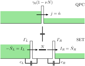
Even though in these experiments, eventually the SET current is determined, it is obvious that the measured quantity is the dot occupation rather than the current. Therefore, the question arises to which extent the detector current correlates with the detected current. To this end, a SET with a QPC in the tunnel regime sketched in Fig. 1 represents a paradigmatic example, despite that most experiments are performed in the limit of an open QPC. A main advantage of considering this model is the absence of backaction and quantum mechanical superpositions, which facilitates the interpretation.

In this work, we derive in Section 2 a stochastic process for the detector coupled to the SET. In this model, the detector does not act back to the SET occupation, so that we can derive in Section 3 the correlation functions of the latter before taking the detector into account. The detector, by contrast, is influenced by the SET and can be described by a Cox process. Its properties are derived in Section 4, while Section 5 focuses on correlations between the subsystems.

2 SET coupled to a tunnel contact

The system sketched in Fig. 1 consists of a SET formed by a single-level quantum dot in contact with electron source and drain. Since double occupation of the SET is inhibited by Coulomb repulsion, spin effects play a minor role and will be ignored. This setup is described by the Hamiltonian

$$H_{\text{SET,leads}}=\epsilon_{0}N+\sum_{\ell,q}V_{\ell,q}(c^{\dagger}c_{\ell,q}+c_{\ell,q}^{\dagger}c)+\sum_{\ell,q}\epsilon_{q}N_{\ell,q},$$ (1)

where $c^{\dagger}$ and $c_{\ell,q}^{\dagger}$ are the usual fermionic creation operators for an electron on the SET and in mode $q$ of lead $\ell=L,R$, respectively, with the corresponding energies $\epsilon_{0}$ and $\epsilon_{q}$ and the occupation numbers $N$ and $N_{\ell,q}$. Tunneling between the SET and the leads is determined by the spectral densities $\Gamma_{\ell}(\epsilon)=(2\pi/\hbar)\sum_{q}|V_{\ell,q}|^{2}\delta(\epsilon-\epsilon_{q})\equiv\Gamma_{\ell}$ which we assume within a wideband limit energy independent.

Within second-order perturbation theory in the SET-lead coupling constants $V_{\ell,q}$, one can obtain a master equation for the occupation probability $P_{N}$ of the SET, where $N=0,1$. For unidirectional transport, i.e., in the limit of large bias voltage, it reads Gurvitz1996a

$$\frac{d}{dt}\begin{pmatrix}P_{0}\\ P_{1}\end{pmatrix}=\begin{pmatrix}-\Gamma_{L}&\Gamma_{R}\\ \Gamma_{L}&-\Gamma_{R}\end{pmatrix}\begin{pmatrix}P_{0}\\ P_{1}\end{pmatrix}\equiv LP,$$ (2)

where the load rate $\Gamma_{L}$ and the unload rate $\Gamma_{R}$ are given by the spectral densities of the respective dot-lead coupling. The current through the left barrier is determined by the load rate times the probability that the SET is empty, $I_{L}=\Gamma_{L}P_{0}$. Vice versa, the current through the right barrier is given by $I_{R}=\Gamma_{R}P_{1}$. Notice that we consider particle currents, i.e, the electrical current is obtained by multiplication with the elementary charge.

According to the Ramo-Shockley theorem Shockley1938a ; Ramo1939a ; Blanter2000a ; Mozyrsky2002a , the experimentally measured current $I$ is the weighted average of the currents through the left and the right tunnel barrier,

$$I=\alpha I_{L}+\beta I_{R}.$$ (3)

The weights $\alpha$ and $\beta$ are determined by the barrier capacitances between the SET and the leads and obey $\alpha+\beta=1$ Blanter2000a ; Mozyrsky2002a . Typically, low-frequency properties, such as the average current or the zero-frequency noise, are the same for both $I_{L}$ and $I_{R}$. Thus in that limit, one may ignore the partition (3) or set for convenience both weights to $1/2$. Here however, we will find that some SET-QPC correlations possess an imaginary part proportional to $\alpha-\beta$.

The charge detector is formed by a point contact in the weak coupling limit which we model by a tunnel Hamiltonian whose transmission depends on the SET occupation Gurvitz1997a ; Braggio2009a

$$\begin{split}H_{\text{QPC}}={}&\sum_{k}\epsilon_{k}c_{k}^{\dagger}c_{k}+\sum_{k^{\prime}}\epsilon_{k^{\prime}}c_{k^{\prime}}^{\dagger}c_{k^{\prime}}\\ &+(1-\tilde{\nu}N)\sum_{kk^{\prime}}T_{kk^{\prime}}(c_{k}^{\dagger}c_{k^{\prime}}+c_{k^{\prime}}^{\dagger}c_{k}).\end{split}$$ (4)

It couples the states $k$ of the left lead to the states $k^{\prime}$ of the right lead via the tunnel matrix element $T_{kk^{\prime}}$, where $c_{k}^{\dagger}$ and $c_{k^{\prime}}^{\dagger}$ are the corresponding fermionic creation operators for electrons with energies $\epsilon_{k}$ and $\epsilon_{k^{\prime}}$. The number operator $N$ in the prefactor of the last term reflects the fact that an electron on the SET reduces the tunnel amplitudes. The strength of this reduction depends on the interaction with the SET which is quantified by the dimensionless parameter $\tilde{\nu}$ .

Since $H_{\text{QPC}}$ commutes with $N$, the charge detector does not directly act back to the SET occupation. Notice that owing to $[H_{\text{QPC}},H_{\text{SET,leads}}]\neq 0$, there is an indirect backaction which, however, is beyond second-order perturbation theory in the SET-lead coupling. Therefore it will not be considered.

In turn, within this level of description, the SET-lead tunneling $V_{\ell,q}$ can be neglected in the computation of the QPC tunnel rates. Thus, we can adopt the golden-rule treatment of Ref. Ingold1992a by which we obtain that an electron in state $k$ of the left lead may tunnel to state $k^{\prime}$ of the right lead with probability $(2\pi/\hbar)|T_{kk^{\prime}}|^{2}\delta(\epsilon_{k}-\epsilon_{k^{\prime}})(1-\tilde{\nu}N)^{2}$. Expressing the probability for the possible initial state in terms of Fermi function and integrating over $\epsilon_{k}$ and $\epsilon_{k^{\prime}}$, we obtain for $N=0$ that the QPC current can be described by a Poisson process Blanter2000a with a rate $\gamma_{0}$ proportional to the QPC bias voltage Ingold1992a . If an electron resides on the SET, i.e. for $N=1$, Coulomb repulsion reduces the tunnel rates according to $\gamma_{0}\to\gamma_{1}\equiv\gamma_{0}(1-\nu)$, where $\nu=\tilde{\nu}(2-\tilde{\nu})$ reflects the detector sensitivity and ideally assumes the value $\nu=1$. Subsuming these two cases, we can conclude that the QPC tunnel process inherits an additional randomness from the SET occupation. In more technical terms, the Poisson process turns into a Cox process with a rate

$$\gamma(t)=\gamma_{0}(1-\nu N(t))$$ (5)

that depends on the two-state process $N(t)$.

3 Charge-current correlations of the SET

The SET described above is a frequently studied example of mesoscopic transport for which most properties can be obtained analytically. In recent years, it has been employed for studying full-counting statistics of the transported electrons, time-dependent correlations Emary2007a , as well as waiting time distributions Brandes2008a . Here by contrast, we are interested in the correlations between the dot occupation and the incoming and the outgoing current.

Let us start by considering basic expectation values. It is straightforward to verify that the stationary solution of the master equation (2) and the average currents read

$$P_{0}^{\text{st}}=\frac{\Gamma_{R}}{2\Gamma},\quad P_{1}^{\text{st}}=\frac{\Gamma_{L}}{2\Gamma},\quad\langle I\rangle=\frac{\Gamma_{L}\Gamma_{R}}{2\Gamma}=\langle I_{L}\rangle=\langle I_{R}\rangle,$$ (6)

where $\Gamma\equiv(\Gamma_{L}+\Gamma_{R})/2$. An interesting observation is that in very asymmetric situations, $\Gamma\approx\max(\Gamma_{L},\Gamma_{R})$, while $\langle I\rangle\approx\min(\Gamma_{L},\Gamma_{R})$.

The master equation (2) provides direct information about the SET only, while the lead degrees of freedom have been traced out. Nevertheless, there exist various ways to obtain information about the statistics of the transported electrons, e.g., by attributing a counting variable to the terms that correspond to the tunnel process of interest. This provides the moment and the cumulant generating function for the lead electrons in the long-time limit Bagrets2003a and for finite frequencies Emary2007a .

Alternatively, one may employ the approach of Refs. Korotkov1994a ; Hanke1995a , which is rather convenient for our purposes. Its cornerstone is the conditional probability $P(N,t|N^{\prime},t^{\prime})$ for having at time $t$ the SET occupation $N$ provided that at an earlier time $t^{\prime}$, it was occupied by $N^{\prime}$ electrons. Since the SET occupation is unique at any time, the conditional probability must fulfill the boundary condition $P(N,t^{\prime}|N^{\prime},t^{\prime})=\delta_{NN^{\prime}}$. Moreover, it obeys the same master equation as the unconditioned probability vanKampen1992a . Therefore, the conditional probability is equivalent to the propagator of the master equation (2), i.e.,

$$P(N,t|N^{\prime},t^{\prime})=\big{[}e^{L(t-t^{\prime})}\big{]}_{NN^{\prime}}\,,$$ (7)

where

$$e^{Lt}=\frac{1}{2\Gamma}\begin{pmatrix}\Gamma_{R}+\Gamma_{L}e^{-2\Gamma t}&&\Gamma_{R}&-\Gamma_{R}e^{-2\Gamma t}\\ \Gamma_{L}-\Gamma_{L}e^{-2\Gamma t}&&\Gamma_{L}&+\Gamma_{R}e^{-2\Gamma t}\end{pmatrix}$$ (8)

can be computed readily by diagonalizing $L$. Notice that the conditional probability (7) is stationary, i.e., it depends only on the time difference $t-t^{\prime}$.

Before considering currents, we compute the auto correlation function of the dot occupation, $\langle N(t)N(t^{\prime})\rangle-\langle N\rangle^{2}$. Since $N$ may assume only the values 0 and 1, the two-time expectation value is given by the probability that the SET is occupied at both times $t$ and $t^{\prime}$. Thus, in terms of the conditional probability and the stationary occupation, it reads $P(1,t|1,t^{\prime})P_{1}^{\text{st}}$. By use of Eqs. (6) and (7), we find $C_{NN}(t-t^{\prime})=(\langle I\rangle/2\Gamma)\exp[-2\Gamma(t-t^{\prime})]$. Via Fourier transformation follows the spectral density

$$C_{NN}(\omega)=\frac{2\langle I\rangle}{\omega^{2}+4\Gamma^{2}}\,.$$ (9)

From the SET master equation (2), we can draw conclusions about the change of the lead electron number in the infinitesimal time interval $[t,t+dt]$, $dN_{R}(t)=I_{R}(t)dt$. This is possible because owing to charge conservation, $dN_{R}(t)=-dN(t)$ for all transitions that physically corresponds to electron tunneling between the SET and the right lead. Consequently, the expectation value $\langle dN_{R}(t)\rangle$ is given by the joint probability that an electron resides on the SET and that in the time interval $[t,t+dt]$, the SET undergoes a transition from $N=1$ to $N=0$. Thus, $\langle dN_{R}(t)\rangle=P(0,t+dt|1,t)P_{1}^{\text{st}}=\langle I\rangle dt$, with the stationary current $\langle I\rangle$ given in Eq. (6).

The correlation between $N$ and $I_{R}$ can be obtained upon noticing that the only trajectory contributing to the expectation value $\langle N(t)\,dN_{R}(t^{\prime})\rangle$ starts with with an electron on the SET at time $t^{\prime}$ which subsequently leaves to the right lead during infinitesimal time $dt^{\prime}$. At time $t$, the SET must be occupied again. The joint probability for this reads $P(0,t+dt|1,t)P(1,t|1,t^{\prime})P_{1}^{\text{st}}$. Subtracting $\langle N\rangle\langle dN_{R}\rangle$ and dividing by $dt$ yields the correlation function $C_{NI_{R}}(t-t^{\prime})=-\langle I\rangle P_{0}^{\text{st}}\exp[-2\Gamma(t-t^{\prime})]$ for $t>t^{\prime}$. For $t<t^{\prime}$, the relevant trajectory starts with electron tunneling to the drain followed by tunneling from the source. This happens with probability $P(1,t|0,t^{\prime}+dt^{\prime})P(0,t^{\prime}+dt^{\prime}|1,t^{\prime})$, so that

$$C_{NI_{R}}(t)=\begin{cases}+\langle I\rangle P_{0}^{\text{st}}e^{-2\Gamma|t|}&\text{for $t<0$},\\ -\langle I\rangle P_{1}^{\text{st}}e^{-2\Gamma t}&\text{for $t>0$}.\end{cases}$$ (10)

By an analogous reasoning for the electron tunneling from the left lead to the SET, we obtain

$$C_{NI_{L}}(t)=\begin{cases}-\langle I\rangle P_{1}^{\text{st}}e^{-2\Gamma|t|}&\text{for $t<0$},\\ +\langle I\rangle P_{0}^{\text{st}}e^{-2\Gamma t}&\text{for $t>0$}.\end{cases}$$ (11)

The anti-correlation between the current and the occupation manifest in the negative sign of $C_{NI_{R}}(t)$ for $t>0$ has the obvious interpretation that the SET is not occupied right after an electron has tunneled to the right lead. In the case of $C_{NI_{L}}(t)$, the minus sign reflects the fact that an electron may tunnel to the SET only when the latter is empty. The by and large anti-symmetric structure as function of time will be discussed below in the context of SET-detector correlations.

Below we will need for the computation of normalized correlation coefficients the auto correlation functions of the incoming and the outgoing currents, $I_{L}$ and $I_{R}$. They can be obtained from the relation $dN_{L}(t)\,dN_{L}(t^{\prime})=I_{L}(t)I_{L}(t^{\prime})dt\,dt^{\prime}$. The only contribution to this expression stems from two source-SET tunnel events, one at time $t$, the other at $t^{\prime}$. For $t>t^{\prime}$ the corresponding joint probability is $P(1,t+dt|0,t)P(0,t|1,t^{\prime}+dt^{\prime})P(1,t^{\prime}+dt^{\prime}|0,t^{\prime})P_{0}^{\text{st}}$. Subtracting $\langle I\rangle^{2}$, adding the shot noise $\langle I\rangle\delta(t-t^{\prime})$, and performing a Fourier transformation, we obtain the known result Korotkov1994a ; Blanter2000a ; Emary2007a ; Brandes2008a

$$S_{I_{L}I_{L}}(\omega)={} S_{I_{R}I_{R}}(\omega)=\frac{\omega^{2}+\Gamma_{L}^{2}+\Gamma_{R}^{2}}{\omega^{2}+(\Gamma_{L}+\Gamma_{R})^{2}}\,\langle I\rangle$$ (12)

$$\equiv{} F_{\text{SET}}(\omega)\,\langle I\rangle,$$ (13)

where the frequency-dependent Fano factor is bounded according to $1/2\leq F_{\text{SET}}(\omega)<1$. For for a derivation of the shot noise term $\langle I\rangle\delta(t-t^{\prime})$ in the spirit of the present calculation, see Ref. Korotkov1994a .

4 Detector current

Charge transport through the QPC in the tunnel limit is a Markov process Blanter2000a , where in our case the rate $\gamma(t)=\gamma_{0}(1-\nu N)$ is a stochastic process as well, see Eq. (5). The state of the detector at time $t$ can be characterized by the number of electrons $n$ that have been tunneling thus far. For unidirectional transport, a direct transition from $n$ is possible only to $n+1$, but not to $n-1$. One can readily write down a master equation for the probability $p_{n}(t,t^{\prime})$ that $n$ electrons have been tunneling between time $t^{\prime}$ and a later time $t$ vanKampen1992a ,

$$\frac{d}{dt}p_{n}(t,t^{\prime})=\gamma(t)\big{[}p_{n-1}(t,t^{\prime})-p_{n}(t,t^{\prime})\big{]}$$ (14)

with the initial condition $p_{n}(t^{\prime},t^{\prime})=\delta_{n,0}$. For $\nu=0$, $\gamma(t)=\text{const}$, so that this equation describes a Poisson process, while otherwise, it constitutes a stochastic process that inherits additional randomness from the SET. It is straightforward to demonstrate that the solution of the master equation (14) is the Poisson-like distribution

$$p_{n}(t,t^{\prime})=\frac{1}{n!}\phi_{t,t^{\prime}}^{n}e^{-\phi_{t,t^{\prime}}}$$ (15)

with the mean number of events during time $t-t^{\prime}$ replaced by the integral

$$\phi_{t,t^{\prime}}=\int_{t^{\prime}}^{t}ds\,\gamma(s)\,.$$ (16)

For the initial time $t^{\prime}=0$, all moments and cumulants of this process can be calculated in a more or less elementary way. In particular, one finds the expectation values

$$\overline{n(t)}={} \phi_{t,0},$$ (17)

$$\overline{n(t)n(t^{\prime})}={} \phi_{t,0}\phi_{t^{\prime},0}+\phi_{\min(t,t^{\prime}),0}.$$ (18)

The overbar denotes the average over only the tunnel contact, while angular brackets will refer to the additional average over the full system including the SET.

For completeness, we sketch the derivation of Eqs. (17) and (18) and refer for a more general treatment to Ref. Bouzas2006a . The average number of transported electrons, Eq. (17), is simply the first moment of the distribution function (15). The two-time expectation value (18) can be defined as $\sum_{n,n^{\prime}}nn^{\prime}p(n,t;n^{\prime},t^{\prime})$, where $p(n,t;n^{\prime},t^{\prime})$ is the joint probability of finding $n^{\prime}$ transported electrons at time $t^{\prime}$ and $n$ electrons at a later time $t$. With the help of Bayes theorem, it can be written as $p(n,t;n^{\prime},t^{\prime})=p(n,t|n^{\prime},t^{\prime})p_{n^{\prime}}(t^{\prime})$, where the conditional probability $p(n,t|n^{\prime},t^{\prime})$ obeys the master equation (14) with the usual boundary condition $p(n,t|n^{\prime},t)=\delta_{n,n^{\prime}}$. Thus, $p(n,t|n^{\prime},t^{\prime})=p_{n-n^{\prime}}(t,t^{\prime})$, so that we find for $n\geq n^{\prime}$ and $t\geq t^{\prime}$ the solution

$$p(n,t;n^{\prime},t^{\prime})=\frac{\exp({-\phi_{t,0}})}{(n-n^{\prime})!\,n^{\prime}!}\,\phi_{t,t^{\prime}}^{n-n^{\prime}}\phi_{t^{\prime},0}^{n^{\prime}}\,.$$ (19)

Evaluating the sum in the above definition yields Eq. (18).

The detector current and its correlation function follow from Eqs. (17) and (18) by time differentiation, which yields expressions that still depend on the absolute time. Only after averaging over the SET variables, they become stationary and read

$$\langle j\rangle={} \gamma_{0}(1-\nu P_{1}^{\text{st}}),$$ (20)

$$C_{jj}(\omega)={} \langle j\rangle+\nu^{2}\gamma_{0}^{2}C_{NN}(\omega),$$ (21)

where the latter is the Fourier representation of $C_{jj}(t-t^{\prime})$. An established measure for the relative noise strength is the frequency-dependent Fano factor

$$F_{\text{QPC}}(\omega)=\frac{C_{jj}(\omega)}{\langle j\rangle}=1+\frac{\nu^{2}\gamma_{0}^{2}C_{NN}(\omega)}{\langle j\rangle}.$$ (22)

Its first term is the usual shot noise which one obtains also for a constant QPC tunnel rate. The second term is the excess noise stemming from the stochastic character of QPC rate. Generally, $F_{\text{QPC}}>1$ which indicates avalanche-like transport due to the switching between high and low detector rates as a consequence of the alternating SET occupation. If the noise enhancement is small compared to the shot noise, the detector current is essentially not affected by the SET, and we expect that no information can be drawn from the measurement. In accordance with this, we will find that the correlation between the SET occupation and the detector current is indeed governed by the Fano factor (22).

5 Detector-SET correlations

From the expectation value (17) together with Eqs. (5) and (16) follows the detector current $\overline{j(t)}=\gamma_{0}-\nu\gamma_{0}N(t)$. Since the first term of this expression is constant, any correlation of $j$ with a SET variable $x$ must stem from the second term and, thus, read

$$C_{jx}=-\nu\gamma_{0}C_{Nx}\,.$$ (23)

Since we are interested in the degree of correlation rather than in absolute values, we focus on the normalized correlation at a given measurement frequency $\omega$ which we define as

$$r_{xy}(\omega)=\frac{C_{xy}(\omega)}{\sqrt{C_{xx}(\omega)\,C_{yy}(\omega)}}\,.$$ (24)

Its absolute value is a figure of merit for the detection quality and in the ideal case is of order unity. In turn, for $|r_{jx}|\ll 1$, the detector current is practically independent of $x$.

5.1 SET charge

By construction, the charge detector is sensitive to the SET charge, which implies that the correlation coefficient $r_{jN}$ must be close to unity at least in some frequency range. Since the QPC current can be expressed in terms of the SET occupation, we can express $C_{jj}$ and $C_{jN}$ by $C_{NN}$. The latter can be eliminated in favor of the frequency-dependent Fano factor (22) so that the correlation coefficient becomes

$$r_{jN}(\omega)=-\sqrt{\frac{F_{\text{QPC}}(\omega)-1}{F_{\text{QPC}}(\omega)}}\,.$$ (25)

It is close to unity if $F_{\text{QPC}}\gg 1$. This means that, as conjectured above, we can acquire information about the SET occupation only if the detector current exhibits significantly super-Poissonian noise.

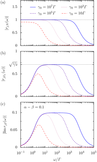
Moreover, this result turns some natural expectations for the measurement process into quantitative statements. Fist, one expects that the time resolution $\tau$ of the detector has some lower limit set by the condition that during time $\tau$, many electrons should flow in order to establish a clear signal. Thus, $\tau\gg 1/\gamma_{0}$ or in terms of the measurement frequency: $\omega\ll\gamma_{0}$. Second, for the specific measurement of the SET occupation, the SET dwell time should be larger than the time resolution, $1/\Gamma\gtrsim\tau$, which together with the above condition yields $\Gamma\ll\gamma_{0}$. The quantitative analysis shown in Fig. 2(a) demonstrates that even for an ideal detector $\nu=1$, in order to find $r_{jN}(\omega)\approx 1$, these inequalities need to be fulfilled by roughly two orders of magnitude, i.e., $\gamma_{0}\gtrsim 100\Gamma$ and $\gamma_{0}\gtrsim 100\omega$.

The Fano factor $F_{\text{QPC}}$ exhibits an interesting asymmetry with respect to the SET tunnel rates. For $\nu\approx 1$ and $\omega=0$, it can be approximated as $F_{\text{QPC}}\approx 1+2\gamma_{0}\Gamma_{L}/\max(\Gamma_{L},\Gamma_{R})^{2}$. Thus, starting from a symmetric situation, the Fano factor remains constant if $\Gamma_{R}$ is reduced, while it becomes smaller upon reducing $\Gamma_{L}$. Nevertheless, as long as $\gamma_{0}$ is sufficiently large, one can achieve in both cases a correlation coefficient close to unity.

Figure 2: (a) Absolute value of the correlation coefficient between the SET occupation and the detector current for various detector rates $\gamma_{0}$, tunnel rates $\Gamma_{L}=\Gamma_{R}=\Gamma$, ideal sensitivity, $\nu=1$, and $\alpha=\beta=1/2$. (b) Absolute value of the correlation coefficient between the SET source current $I_{L}$ and the detector current for the same parameters. (c) Imaginary part of the correlation between detector current and the total SET current for Ramo-Shockley coefficients with $|\alpha-\beta|=0.1$.

5.2 Source and drain currents

The correlation between the source current $I_{L}$ and the detector current follows by inserting (11) into (23). Unless $\Gamma_{L}=\Gamma_{R}$, the resulting expression is neither symmetric nor anti-symmetric, so that the spectral density is complex and reads

$$C_{jI_{L}}(\omega)={} \nu\gamma_{0}\langle I\rangle\,\frac{-i\omega+\Gamma_{L}-\Gamma_{R}}{\omega^{2}+(\Gamma_{L}+\Gamma_{R})^{2}}$$ (26)

$$={} C_{jI_{R}}^{*}(\omega).$$ (27)

The second equation represents the corresponding expression for the SET drain and is obtained accordingly. For a symmetric SET with $\Gamma_{L}=\Gamma_{R}$, this correlation function vanishes in the limit $\omega\to 0$ in accordance with the asymmetric behavior as function of time, cf. Eqs. (10) and (11). This implies that the corresponding correlation for the long-time limit of the counting statistics vanishes as well, $\lim_{t\to\infty}\langle n,N_{L/R}\rangle=0$.

A more detailed analysis of Eq. (26) reveals that the correlation coefficient $r_{jI_{L}}$ may assume the appreciable value $\sqrt{1/2}$. The limitation is due to the fact that the detector is sensitive to both the source and the drain current. Because tunnel events at source and drain alternate, they are not statistically independent. Thus, there is no contradiction in $|r_{jI_{L}}|$ exceeding the value $1/2$. We depict in Fig. 2(b) a quantitative analysis for the symmetric situation. It shows that also here the condition $\gamma_{0}\geq 100\Gamma,100\omega$ must be fulfilled in order to achieve a significant correlation. Moreover, at frequencies below the SET rate, $\omega\lesssim\Gamma$, both currents become statistically independent, because the detector “sees” merely the average population of the SET.

5.3 Ramo-Shockley current

According to the Ramo-Shockley theorem, the experimentally relevant SET current is the one given by Eq. (3), i.e., $I=\alpha I_{L}+\beta I_{R}$. From charge conservation follows $-I_{L}+\dot{N}+I_{R}$, while $C_{\dot{N}\dot{N}}(\omega)=\omega^{2}C_{NN}(\omega)$. This yields for the total current the correlation function Blanter2000a

$$C_{II}(\omega)={} \alpha C_{I_{L}I_{L}}+\beta C_{I_{R}I_{R}}-\alpha\beta\omega^{2}C_{NN}$$ (28)

$$={} \frac{(1-2\alpha\beta)\omega^{2}+\Gamma_{L}^{2}+\Gamma_{R}^{2}}{\omega^{2}+(\Gamma_{L}+\Gamma_{R})^{2}},$$ (29)

which we need for normalizing $C_{jI}=\alpha C_{jI_{L}}+\beta C_{jI_{R}}$. Writing $C_{jI_{\ell}}$ for $\ell=L,R$ in terms of $C_{NI_{\ell}}$, see Eq. (23), we obtain

$$C_{jI}(\omega)=\nu\gamma_{0}\langle I\rangle\,\frac{\Gamma_{L}-\Gamma_{R}-i\omega(\alpha-\beta)}{\omega^{2}+4\Gamma^{2}}\,.$$ (30)

Interestingly enough, $C_{jI}$ depends on the difference of the tunnel rates, $\Gamma_{L}-\Gamma_{R}$, and on the difference of the Ramo-Shockley coefficients, $\alpha-\beta$. It vanishes for a completely symmetric setup. Thus, we face the surprising situation that the realization of the stochastic process $I(t)$ can be determined by measuring $j(t)$, despite that both quantities are uncorrelated. This underlines that the determination of the SET current by charge detection must rely on implicit knowledge about the transport process, in the present case its unidirectionality.

An intuitive explanation for the lack of correlations in the symmetric case can be derived from the fact that unidirectional transport through a symmetric SET can be mapped to a Poisson process with half charges Elattari2002a . The events of this process are electron tunnelings from the source to the SET and from the SET to the drain, which both contribute with a half electron to the total current $I$. The waiting time between two subsequent events is exponentially distributed with equal mean time Brandes2008a . Thus, with any of the two tunnel events, the detector may switch in either direction, from on to off or back. Then for symmetry reasons the correlation between the detector and the total SET current $I$ must vanish.

Going beyond the symmetric situation, we find that the imaginary part $\mathop{\mathrm{Im}}C_{jI}(\omega)$ is finite and proportional to the difference of the Ramo-Shockley coefficients, $\alpha-\beta$. This in principle allows one to determine the ratio of the barrier capacitances $c_{L}$ and $c_{R}$. Analyzing the correlation coefficient $r_{jI}(\omega)$ for $|\alpha-\beta|\ll 1$ reveals that such measurement is possible under the following conditions. First, as for all other SET-detector correlations, the Fano factor $F_{\text{QPC}}$ must lie significantly above the Poissonian value which requires $\gamma_{0}\gtrsim 100\Gamma$. Moreover, the measurement frequency must be so large that the SET is not in its zero-frequency limit, $\omega\gtrsim\Gamma$. Then $\mathop{\mathrm{Im}}r_{jI}\approx|\alpha-\beta|$ in an intermediate frequency range. The data shown in Fig. 2(c) visualize this estimate. In recent experiments on monitoring SET currents Gustavsson2007a ; Fujisawa2006a ; Fricke2007a , the relevant frequencies were of the order 10 kHz. In this regime, it is possible to record time-resolved measurements and to subsequently obtain the frequency dependent correlation coefficient by numerical data processing.

6 Discussion

We have studied correlations between the currents of a charge detector interacting capacitively with a SET. As a simple fully classical model, we have employed as detector a QPC in the weak-tunneling limit. Then electron transport through the detector constitutes a Cox process, i.e., a Poisson with a stochastic rate for which all correlation function can be obtained analytically.

The fundamental correlation upon which the measurement idea is based, is the one between the detector and the SET occupation. It grows with the Fano factor of the detector current, while no particular features of the SET enter. The need for super Poissonian detector noise indicates the requirement for switching between large periods of conducting and non-conducting behavior. On the quantitative level, on the order of 100 electrons should flow during a conducting period. Then the current noise of the detector exhibits significant bunching.

For a symmetric SET whose tunnel barriers possess equal tunnel rates and equal Ramo-Shockley factors, the detector current is independent of the total SET current, i.e, the average between the source and drain current. This can be understood by mapping of the symmetric SET to a Poisson process with “half charges”, because in this picture both source-SET tunneling and SET-drain tunneling contribute equally to the total current. Beyond the fully symmetric situation, correlations emerge. Most interesting is a contribution proportional to the difference of the Ramo-Shockley coefficients which, thus, in principle can be measured. In contrast to the total current, the source current and the drain current correlate with the detector even for a symmetric setup. The correlation is limited to $\sqrt{1/2}$, which still is an appreciable value.

In conclusion, already a simple model for mesoscopic charge monitoring exhibits interesting correlations that should be measurable readily with present setups. Many more may be predicted for coupled conductors that allow for quantum features such as electrons in delocalized orbitals.