Phase transitions of the $q$-state Potts model on multiply-laced Sierpinski gaskets

Abstract

We present an exact solution of the $q$-state Potts model on a class of generalized Sierpinski fractal lattices. The model is shown to possess an ordered phase at low temperatures and a continuous transition to the high temperature disordered phase at any $q\geq 1$. Multicriticality is observed in the presence of a symmetry-breaking field. Exact renormalization group analysis yields the phase diagram of the model and a complete set of critical exponents at various transitions.

I Introduction

The study of models on hierarchically organized lattices has enriched our understanding of critical phenomena at phase transitions Berker ; Gefen79 ; Griffiths81 ; Derrida83 ; DeSimoi . In many cases, the renormalization group (RG) transformation of the partition function can be carried out exactly Dhar77 ; Berker ; Griffiths84 . Exhaustive search of the RG fixed points and a complete characterization of the flow in the Hamiltonian space then become possible. Various conjectures on the universality of the critical exponents and their dependence on dimensionality and other model parameters can be tested. The intuition gained from the study can be used to guide the interpretation of numerical results and experiments.

In this work, we analyze an exact solution of the $q$-state Potts model Wu on a class of fractal lattices with and without a symmetry-breaking field. These lattices, first introduced by Menezes and MagalhãsesMenezes92 , are simple extensions of the well-known Sierpinski gasket. They can be constructed iteratively following the scheme shown in Fig. 1. The Potts model (including the Ising model at $q=2$) on the original Sierpinski gasket does not order except at zero temperature Gefen79 ; Gefen83 ; Luscombe ; Borjan . This may seem surprising at first sight since the gasket has a fractal dimension $d_{\rm f}=\ln 3/\ln 2=1.58$ greater than the lower critical dimension $d_{\rm lc}=1$ from field theory. The puzzle was partially resolved by Gefen, Mandelbrot and Aharony Gefen79 ; Gefen84 who noticed that, in addition to the fractal dimension, other topological features of a lattice also affect the existence of a finite temperature transition and its critical properties.

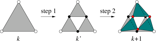
Figure 1: (Color online.) Iterative construction of the multiply-laced Sierpinski gasket at $m=2$ in two steps and the renormalization group transformation. Potts spins at the corners of the triangle (open circles) are used to define the restricted partition functions at a given order $k$. Solid circles indicate the internal vertices to be integrated out to yield the renormalized interactions.

The laced Sierpinski gasket can be considered as a hybrid of the Sierpinski gasket and the Berker lattice, which does allow a finite temperature transition with a Potts Hamiltonian Berker ; Griffiths84 . As in the case of the Berker lattice, the coordination number of corner sites on the lattice grows with iteration. Presence of such vertices gives rise to a hierarchical set of “integration points” that mediate order among subsystems at low temperatures despite their tenuous contact. We construct the phase diagram and calculate the critical properties based on exact RG transformations derived from previous work by Borjan et al.Borjan . Interestingly, when a symmetry-breaking field is introduced, we observe multicritical behavior and a line of continuous transition between two disordered phases.

The paper is organized as follows. The fractal lattice and the Potts model is introduced in Sec. 2. In Sec. 3 we present the iterative relations for the partition function and discuss topological features of the RG trajectories under the mapping, including the relevant fixed points. Section 4 contains calculations of the phase diagram and the critical exponents. A brief summary is presented in Sec. 5.

II Potts model on laced Sierpinski gasket

Figure 1 shows the iterative construction of the fractal lattice in two steps. In the first step, the triangle at a given order $k$ is triplicated and linked together at the three $(k+1)$th order internal vertices (solid circles). In the second step, the structure is replicated $m$-fold and then laced at the three $(k+1)$th order corner vertices (open circles) to form a $(k+1)$th order triangle. The zeroth order triangle is chosen to be a stack of $m$ unit triangles laced at the three corner sites. Each pair of sites are $m$-tuply connected.

Let $N_{k},B_{k}$ and $T_{k}$ be the total number of sites, bonds and basic triangles on a $k$th order triangle, respectively. From the above definition, we have $N_{k+1}=3mN_{k}-6m+3,B_{k+1}=3mB_{k}$ and $T_{k+1}=3mT_{k}$, with $N_{0}=3,B_{0}=3m$ and $T_{0}=m$. Hence

$$N_{k}={(3m)^{k+1}-1\over 3m-1}+2,B_{k}=(3m)^{k+1},T_{k}=m(3m)^{k}.$$ (1)

Since the linear size of the triangle doubles upon each iteration, the fractal dimension of the lattice is given by $d_{\rm f}=\ln(3m)/\ln 2$.

The coordination number or the degree of a $k$th order corner vertex is given by $C_{k}=2m^{k+1}$. The coordination number of an internal vertex at the same order is $D_{k}=2C_{k-1}=4m^{k}$. On a fractal lattice of order $n$, there are three $n$th order corner vertices. The number of $k$th order internal vertices can be calculated from the iterative relation $N_{n,k}=3mN_{n,k+1}$, with $N_{n,n}=3m$. Hence $N_{n,k}=(3m)^{n-k+1}$. It is easily verified that $N_{n}=3+\sum_{k=1}^{n}N_{n,k}$ and $B_{n}={3\over 2}C_{n}+{1\over 2}\sum_{k=1}^{n}N_{n,k}D_{k}$. Note that the number of internal vertices with a given degree $D$ satisfies $N(D)\sim D^{-\kappa}$ where $\kappa=\ln(3m)/\ln(m)$. For the Sierpinski gasket at $m=1$, all internal vertices have the same coordination number $D=4$.

We now assign a Potts variable $\sigma_{i}=0,1,\ldots,q-1$ to each of the lattice sites. The energy of a Potts configuration $\{\sigma_{i}\}$ is given by,

$${\cal H}=-J\sum_{\langle ij\rangle}\delta(\sigma_{i},\sigma_{j})-H\sum_{i}\delta(\sigma_{i},0).$$ (2)

The first sum extends over all pairs of sites connected by a bond, while the second sum introduces a symmetry-breaking field that favors or disfavors a selected Potts spin state $\sigma=0$. Here $\delta(\sigma,\sigma^{\prime})=1$ if $\sigma=\sigma^{\prime}$ and 0 otherwise. In this work we shall restrict ourselves to the ferromagnetic case at $J>0$.

Model (2) is not invariant under the RG transformation discussed below. However, it can be recast in the form of an invariant model that contains the one-spin term $H$ and a set of three-spin (which includes the pair-wise) interactions on a triangle. Making one spin state (e.g., $\sigma=0$) special, there are altogether seven non-symmetry-related three-spin configurations as shown in Fig. 2. At a given temperature $T$, the three-spin interactions can be expressed in terms of Boltzmann weights $\{Z_{\alpha}\}$ for the triplet configurations Borjan . The one-spin term is represented by a weight $v=\exp(H/T)$ assigned to all internal sites in the state $\sigma=0$. A restricted partition function $Z_{\alpha,k}$ of the fractal lattice at order $k$ is obtained by summing over spins on all internal sites, whereas spins at the three corner sites define the label $\alpha$ according to the scheme shown in Fig. 2.

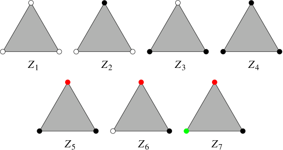
Figure 2: (Color online.) Seven non-symmetry-related three-spin configurations and the associated Boltzmann weights (or restricted partition functions). Open circles represent spins in the selected state $\sigma=0$. Solid circles represent spins in the remaining $q-1$ states distinguished by color.

III Iterative calculation of the partition function and the renormalization group flow

The partition function of the Potts model with three-spin interactions can be computed exactly by following the two-step construction of Fig. 1. In the first step, $\{Z^{\prime}_{\alpha}\}$ on the lattice $k^{\prime}$ are obtained from $\{Z_{\alpha}\}$ by summing over spins on the three internal sites (solid circles). The mapping $\{Z_{\alpha}\}\rightarrow\{Z^{\prime}_{\alpha}\}$ for general $q$ was worked out by Borjan et al., where $v$ enters as a parameter of the RG transformation Borjan ; note1 . In the second step, each of the seven weights are replicated as $Z^{\prime}_{\alpha}\rightarrow\tilde{Z}_{\alpha}=(Z^{\prime}_{\alpha})^{m}$.

To illustrate the procedure, we consider first the symmetric case where the $\sigma=0$ state is made identical to the other $q-1$ states, i.e., $Z_{1,0}=Z_{4,0}$, $Z_{2,0}=Z_{3,0}=Z_{5,0}$, $Z_{6,0}=Z_{7,0}$, and $v=1$. This includes model (2) at $H=0$. The RG transformation defines a two-dimensional map for the variables $x\equiv Z_{5}/Z_{4}$ and $y\equiv Z_{7}/Z_{4}$. Let $z_{\alpha}\equiv Z^{\prime}_{\alpha}/Z_{4}^{3}$, the general iterative relations of Ref. Borjan reduces to:

$$z_{4}(x,y) = 1+(q-1)x^{2}(3+4x)$$

$$+(q-1)(q-2)y\left[3x^{2}+3xy+(q-3)y^{2}\right],$$

$$z_{5}(x,y) = x+4x^{2}+3x^{3}$$ (3)

$$+(q-2)\left(2xy+y^{2}+5x^{3}+8x^{2}y+3xy^{2}\right)$$

$$+(q-2)(q-3)y\left[x^{2}+7xy+(q-3)y^{2}\right],$$

$$z_{7}(x,y) = 3x^{2}+6xy+8x^{3}+9x^{2}y+y^{3}$$

$$+(q-3)\left(3y^{2}+x^{3}+21x^{2}y+9xy^{2}+3y^{3}\right)$$

$$+(q-3)(q-4)y^{2}[9x+(q-2)y].$$

The new ratios of the restricted partition functions after one iteration are then given by,

$$\tilde{x} = \phi(x,y)\equiv\Bigl{[}{z_{5}(x,y)\over z_{4}(x,y)}\Bigr{]}^{m},$$

$$\tilde{y} = \psi(x,y)\equiv\Bigl{[}{z_{7}(x,y)\over z_{4}(x,y)}\Bigr{]}^{m}.$$

Specializing on the model (2) at $H=0$, we have $Z_{4,0}=\exp(3mJ/T),Z_{5,0}=\exp(mJ/T)$, and $Z_{7,0}=1$. The starting values of the iteration are $x_{0}=Z_{5,0}/Z_{4,0}=\exp(-2mJ/T)$ and $y_{0}=Z_{7,0}/Z_{4,0}=\exp(-3mJ/T)$. Successive applications of Eqs. (III) and (LABEL:tilde-xy) yield the ratios $x_{k+1}=\phi(x_{k},y_{k})$ and $y_{k+1}=\psi(x_{k},y_{k})$.

The full partition function on the $n$th order triangle is obtained from the restricted partition functions,

$$Z_{k}=q\left[1+3(q-1)x_{k}+(q-1)(q-2)y_{k}\right]Z_{4,k},$$ (5)

where $Z_{4,k}$ satisfies the iterative relation,

$$Z_{4,k}=[z_{4}(x_{k-1},y_{k-1})Z_{4,k-1}^{3}]^{m}.$$ (6)

To compute the free energy $F_{k}=-T\ln Z_{k}$, we obtain from Eq. (6),

$$\ln Z_{4,k} = m\ln z_{4}(x_{k-1},y_{k-1})+3m\ln Z_{4,k-1}$$ (7)

$$= B_{k}J/T+\sum_{n=0}^{k-1}T_{k-n-1}\ln z_{4}(x_{n},y_{n}).$$

The free energy per unit triangle in the infinite size limit is thus expressed as,

$$f(T)\equiv\lim_{k\rightarrow\infty}{F_{k}\over T_{k}}=-3J-T\sum_{n=0}^{\infty}(3m)^{-n-1}\ln z_{4}(x_{n},y_{n}).$$ (8)

The mapping defined by Eqs. (III) and (LABEL:tilde-xy) has two trivial fixed points at ${\rm L}=(0,0)$ and ${\rm H}=(1,1)$ on the $(x,y)$-plane, corresponding to the ordered and disordered phases, respectively. As noted previouslyGefen83 , on the Sierpinski gasket at $m=1$, the mapping at small $x$ yields,

$$\tilde{x}\approx x+4x^{2},$$ (9)

which grows under the iteration. Therefore the low temperature fixed point L is unstable and no finite temperature transition is expected.

For $m>1$, we have $\phi(x,y)\simeq x^{m}$ at small $x$ which turns L into a stable fixed point. Consequently, the Potts model on such a lattice is ordered at sufficiently low temperatures Menezes92 . A third fixed point ${\rm C}=(x_{c},y_{c})$ emerges and controls the critical properties at the transition to the high temperature disordered phase. Figure 3 shows the flow structure of the map at $m=2$ and $q=3$ which is representative of the general situation. The thick solid line is the critical manifold that separates the $(x,y)$-plane into two regions. Below this line, the mapping carries the system to the low temperature fixed point L. Hence this part of the parameter space is associated with the ordered phase. Above the line, the mapping carries the system to the high temperature fixed point H and the system is disordered. On the critical manifold, the mapping carries the system to the hyperbolic fixed point C.

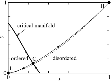
Figure 3: Fixed points (solid circles) and invariant manifolds (solid lines) of the renormalization group transformation at $m=2$ and $q=3$. The critical manifold (thick solid line) divides the parameter space into high and low temperature regions. The dashed line given by $y=x^{3/2}$ corresponds to the Potts model (2) at $H=0$.

In the neighborhood of the fixed point C, the mapping can be well approximated by a linearized version applied to $\delta x_{k}\equiv x_{k}-x_{c}$ and $\delta y_{k}\equiv y_{k}-y_{c}$,

$$\left(\begin{array}[]{c}\delta x_{k+1}\\ \delta y_{k+1}\end{array}\right)=\left(\begin{array}[]{cc}\partial_{x}\phi&\partial_{y}\phi\\ \partial_{x}\psi&\partial_{y}\psi\end{array}\right)\left(\begin{array}[]{c}\delta x_{k}\\ \delta y_{k}\end{array}\right),$$ (10)

where the derivatives are evaluated at $(x_{c},y_{c})$. Diagonalization of the matrix yields two eigenvalues $\lambda_{1}=\lambda_{T}>1$ and $\lambda_{2}<1$ that describe the expansion and contraction rates along the unstable and stable manifolds of the hyperbolic fixed point C, respectively.

More generally, using $Z_{4}$ as the normalization factor, the RG transformation applied to the seven restricted partition functions yields a nonlinear map in six dimensions spanned by $g_{\alpha}\equiv Z_{\alpha}/Z_{4}$. At $v=1$, the symmetric case defines a two-dimensional invariant manifold of the mapping, with L, H and C the three fixed points on this manifold. By tracing the RG flow along the unstable directions emanating from these points, we obtain a total of 9 fixed points as listed in Table 1. Also given in the table is the number of unstable directions $n_{\rm u}$ (known as the codimension) and the maximum eigenvalue $\lambda_{\rm m}$ of the linearized map at each fixed point.

Figure 4 illustrates schematically the RG flow between the fixed points. Points labelled by L^′, C^′, H^′ and L, C^′′, H^′′ lie on the decoupled manifold with $g_{2}=g_{3}=g_{6}=0$. In this case, $\tilde{Z}_{1}=Z_{1}^{3m}$ transforms by itself. The remaining three weights $Z_{4},Z_{5}$ and $Z_{7}$ transform according to Eqs. (III) and (LABEL:tilde-xy) with the replacement $q\rightarrow q^{\prime}=q-1$. The critical fixed point of the $(q-1)$-state Potts model is denoted by $(x^{\prime}_{c},y^{\prime}_{c})$. At criticality, $Z^{\prime}_{4}$ grows by a factor $(z^{\prime}_{4,c})^{m}$ upon each iteration.

Table 1: Fixed points of the RG transformation at $v=1$.

	$g_{1}$	$g_{2}$	$g_{3}$	$g_{5}$	$g_{6}$	$g_{7}$	$n_{\rm u}$	$\lambda_{\rm m}$
C	1	$x_{c}$	$x_{c}$	$x_{c}$	$y_{c}$	$y_{c}$	3	$\lambda_{H}$
H	1	1	1	1	1	1	1	$m$
C′′	$(z^{\prime}_{4,c})^{m\over 3m-1}$	0	0	$x^{\prime}_{c}$	0	$y^{\prime}_{c}$	2	$3m$
H′′	$(q-1)^{3m\over 3m-1}$	0	0	1	0	1	1	$3m$
L	1	0	0	0	0	0	1	$3m$
C′	0	0	0	$x^{\prime}_{c}$	0	$y^{\prime}_{c}$	1	$\lambda^{\prime}_{T}$
L′	0	0	0	0	0	0	0
H′	0	0	0	1	0	1	0
G	$\infty$	$\infty$	$\infty$	0	$\infty$	0	0

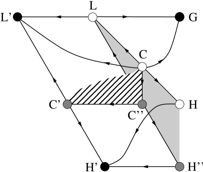
Figure 4: Topological organization of selected fixed points and invariant manifolds under the renormalization group transformation at $v=1$. Solid circles in black are stable fixed points associated with the three bulk phases, separated by the shaded and cross-hatched surfaces that represent first order and continuous transitions, respectively. Open circles lie on the invariant manifold where all $q$ spin states are identical.

The above RG flow topology is largely preserved in a non-zero field $H$. The decoupled manifold at $g_{2}=g_{3}=g_{6}=0$ is invariant under the RG transformation at any $v$. Among the two fixed points not on this manifold, H is always a fixed point of the transformation. The point C survives when $H\neq 0$, but its location shifts with the broken symmetry.

The structure of the RG flow as shown in Fig. 4 is reminiscent of the two-dimensional site-diluted three-state Potts model for the physisorption of Kr on graphite studied by Berker et al. Berker78 The three globally stable fixed points L^′, H^′ and G each represent a “bulk phase”: L^′ for the $(q-1)$-state ordered or in-registry solid phase, H^′ for the $(q-1)$-state disordered or liquid phase, and G for the vacancy ($\sigma=0$) dominated gas phase. The shaded surface in Fig. 4 indicates the phase boundary between the condensed (L^′ and H^′) and gaseous (G) phases. This transition is first order except on the line CH, to be discussed below. On the other hand, transition between the ordered and disordered condensed phases (cross-hatched surface in Fig. 4), controlled by the $(q-1)$-state hyperbolic fixed point C^′, is continuous.

IV Phase diagram of the Potts model and critical exponents

The phase diagram of the Potts model defined by (2) follows from the general topological structure of the renormalization group flow presented in the previous section. As usual, the nature of ordering in the system at a given $T$ and $H$ is determined by which of the three fixed points L^′, H^′ and G the RG transformation carries the set of reduced partition functions to. From symmetry considerations, the phase associated with G occupies the quadrant at $H>0$. On the $H<0$ side, an order-disorder transition among the $q-1$ favored Potts states takes place at a temperature $T_{c}(H)$. The transition temperature at a given $H$ can be determined numerically by noting that the system flows to L^′ for $T<T_{c}(H)$ but to H^′ for $T>T_{c}(H)$ under successive RG transformations. Note that this transition is absent in the special case $q=2$.

Figure 5 shows the phase diagram of the Potts model for the representative case $q=3$ and $m=2$. In the absence of the symmetry-breaking field (i.e., $H=0$), spontaneous ordering occurs for $T<T_{\rm bc}\simeq 2.8919$ with $q$-fold degeneracy. A positive (negative) $H$ selects (de-selects) the $\sigma=0$ state. Thus, as in the case of the Ising model at $q=2$, the line at $H=0$, $T<T_{\rm bc}$ (solid line in Fig. 5) becomes a first order transition line on the $T$-$H$ plane. The order-disorder transition continues on the $H<0$ side (dashed line in Fig. 5) and joins the line of first order transition tangentially at the bicritical point $(T_{\rm bc},H=0)$Fisher_Nelson . Furthermore, the gas and the $(q-1)$-state disordered phases are separated by a continuous transition on the high temperature side.

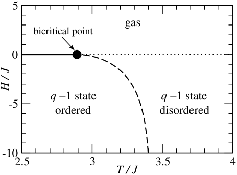
Figure 5: Phase diagram of the Potts model (2) at $m=2$ and $q=3$. Lines of first order (solid) and continuous (dashed and dotted) transitions meet at the bicritical point $H=0$, $T=T_{\rm bc}$.

We now turn to the calculation of the critical exponents that describe the singular behavior of various thermodynamic quantities at the continuous phase transitions. The standard RG procedure allows them to be computed from the eigenvalues of the linearized map at the appropriate fixed points. For example, the order-disorder transition at $H<0$ (dashed line in Fig. 5) is governed by the fixed point C^′ which has a single unstable direction with an eigenvalue $\lambda^{\prime}_{T}(q)\equiv\lambda_{T}(q-1)$. In the neighborhood of the transition point $T=T_{c}(H)$, the free energy contains a singular part $f_{s}\sim|T-T_{c}(H)|^{2-\alpha^{\prime}}$. The standard scaling analysis yields the specific heat exponent $\alpha^{\prime}=2-\ln(3m)/\ln\lambda^{\prime}_{T}$ for the $(q-1)$-state Potts model, independent of $H$.

The first order transition at $H=0,T<T_{\rm bc}$ is governed by the fixed point L. The usual scaling argument suggests that the singular part of the free energy behaves as $f_{s}\sim|H|^{1+1/\delta}$, where $1+1/\delta=\ln d_{f}/\ln\lambda$, with $\lambda$ being the eigenvalue for the unstable direction of the RG flow. At L, $\lambda=3m=d_{f}$ gives $\delta=\delta_{\rm L}=\infty$, hence

$$f_{s}\sim|H|,\qquad(T<T_{\rm bc}).$$ (11)

Equation (11) can also be derived from the jump in the fraction $p_{0}$ of vertices in the $\sigma=0$ state across the transition line. At $H=0$, we have “phase-coexistence” of the $q$ spontaneous symmetry-breaking states, each favoring a particular Potts state whose fraction on the lattice $p(T)>1/q$. A positive field $H$ selects the $\sigma=0$ state with $p_{0}=p(T)$. On the other hand, a negative $H$ de-selects the $\sigma=0$ state, yielding $p_{0}=[1-p(T)]/(q-1)$. In each case, the free energy changes from its $H=0$ value by an amount $\Delta f=-Hp_{0}$ per vertex. The jump in $p_{0}$ gives rise to the singularity in the free energy above.

For $T>T_{\rm bc}$, dependence of the free energy on $H$ is controlled by the RG flow near the fixed point H. Table 1 gives $\lambda=m$ and hence $\delta=\delta_{\rm H}=1/[\ln(3m)/\ln(m)-1]=\ln m/\ln 3$. Consequently,

$$f_{s}\sim|H|^{1+(\ln 3/\ln m)},\qquad(T>T_{\rm bc}).$$ (12)

Such a singular behavior on the high temperature side is quite unusual. The common notion is that the disordered system consists of statistically independent subsystems of finite size. Since the free energy of each subsystem is analytic in the controlling parameters $T$ and $H$, the free energy of the system as a whole should be analytic as well. However, examining Eq. (2) more closely, we find an interesting possibility. Consider a $k$th order vertex and its $C_{k}=2m^{k+1}$ neighbors. A positive external field $H>0$ generates an excess probability of order $H$ for each neighboring spin to be in the $\sigma=0$ state. This gives rise to an effective field $H_{{\rm eff},k}\sim HC_{k}\simeq Hm^{k}$ at the vertex in question from the ferromagnetic couplings, which grows exponentially with $k$. Setting $H_{\rm eff}=T$ yields a critical value $k_{c}=-\ln(H/T)/\ln m$. Vertices with $k>k_{c}$ are completely ordered. Contribution to the free energy per triangle from these vertices is estimated to be $f_{s}\sim T_{k_{c}}^{-1}H_{{\rm eff},k_{c}}\sim(3m)^{-k_{c}}\sim H^{\ln(3m)/\ln m}$ which agrees with Eq. (12).

We now consider the most complex situation near the bicritical point at $H=0,T=T_{\rm bc}$. The RG flow is controlled by the fixed point C which has three unstable directions as shown in Fig. 4. In terms of the scaling fields $t=(T-T_{\rm bc})/T_{\rm bc}$ along CH, $H$ along CG, and $H_{C}$ along CC^′′, the singular part of the free energy is expected to satisfy the scaling,

$$f_{\rm s}(t,H,H_{C})=b^{-d_{\rm f}}f_{\rm s}(b^{y_{T}}t,b^{y_{H}}H,b^{y_{C}}H_{C}),$$ (13)

where $b$ is an arbitrary scaling factor. The scaling exponents $y_{a}$ are related to the eigenvalues $\lambda_{a}$ of the linearized map through $y_{a}=\ln\lambda_{a}/\ln 2$. For the model defined by Eq. (2), $H_{C}$ can be expressed as a linear combination of $t$ and $H$ but since $H_{C}=0$ when $H=0$, we may write $H_{C}=H$. With the choice $b=|t|^{-1/y_{T}}$, Eq. (13) takes a more suggestive form,

$$f_{\rm s}(t,H)=|t|^{2-\alpha}{\cal F}_{\pm}\Bigl{(}{H\over|t|^{\Delta}},{H\over|t|^{\phi}}\Bigr{)},$$ (14)

where the subscript ’$\pm$’ indicates the sign of $t$. Here $\alpha=2-\ln(3m)/\ln(\lambda_{T})$, $\Delta=\ln\lambda_{H}/\ln\lambda_{T}$, and $\phi=\ln\lambda_{C}/\ln\lambda_{T}$ are the specific heat, gap, and crossover exponents, respectively.

Figure 6 shows the numerically computed eigenvalues $\lambda_{H},\lambda_{T}$, $\lambda_{C}$ and the exponents $\alpha,\Delta,\phi$ at $m=2$ but different $q$ values. It is evident that $\lambda_{H}>\lambda_{T}>\lambda_{C}$ and $\Delta>1>\phi$ for all $q$. Dominance of the symmetry-breaking field renders most of the neighborhood of the bicritical point to be occupied by either the $(q-1)$-state ordered phase at $H<0$ or the gas phase at $H>0$. The $(q-1)$-state disordered phase appears in a narrow power-law wedge on the $H<0$ side, bounded below by the transition line $H=H_{c}(T)\simeq-At^{\Delta}$. Within this phase, $H/t^{\phi}\leq At^{\Delta-\phi}\rightarrow 0$ as $t\rightarrow 0$. The scaling function ${\cal F}_{+}(u,w)$ in Eq. (14) is singular on the two transition lines at $u=0$ and $u=-A$, respectively. In the latter case, the scaled variable $w=H/t^{\phi}$ controls the crossover from the $q$-state to the $(q-1)$-state Potts criticality. Details will not be elaborated here.

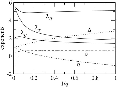
Figure 6: Eigenvalues $\lambda_{H},\lambda_{T}$ and $\lambda_{C}$ associated with the three unstable directions of the renormalization group flow at C against $1/q$. Here $m=2$. Also shown are the specific heat exponent $\alpha$ (dashed line), the gap exponent $\Delta$ (dotted line), and the crossover exponent $\phi$ (dash-dotted line).

At large $q$ values, one may approximate the mapping near C with $\phi(x,y)\simeq\psi(x,y)\simeq(qy)^{3m}$ which yields $x_{c}\simeq y_{c}\simeq q^{-3m/(3m-1)}$. Consequently, $\lambda_{T}(q\rightarrow\infty)=3m$, in agreement with the trend seen in Fig. 6. In this limit, C eventually merges with L, yielding $\lambda_{H}=3m$ as well. Both $\alpha$ and $\Delta$ approach 1. The magnetization exponent $\beta=2-\alpha-\Delta\rightarrow 0$. We have checked that the above behavior is quite general for any $m>1$.

V Summary

In this paper, we analyzed in detail solution of the Potts model on a fractal lattice that has a low temperature ordered phase. Compared to the Sierpinski gasket at $m=1$, the coordination number of vertices at the corners of the fractal triangle with $m>1$ grows with lattice size. Thus our findings are consistent with previous understanding that a finite $T_{c}$ requires sufficiently strong connectivity on the fractal lattice.

Exact renormalization group transformation of the restricted partition functions is presented here with the help of previous work by Borjan et al.Borjan Although the mapping in the six-dimensional space contains many fixed points and invariant manifolds, a relatively simple RG flow diagram is obtained. The flow is mainly defined by three stable fixed points, each representing a bulk phase with a distinct symmetry or broken symmetry. The topology of the RG flow is robust against the lattice geometry parameter $m$ and the number of Potts states $q$. By combining analytical and numerical approaches, we have computed the phase diagram of the model and a complete set of critical exponents for the transitions, including those at the bicritical point, based on the standard RG framework.

It is worth noting that, on the laced Sierpinski gasket, transition to the high temperature disordered phase is continuous for all $q$ values. Previously, solution of the Potts model on the Berker lattice also yielded continuous transitions with a specific heat exponent $\alpha(q)$ that approaches 1 in the limit $q\rightarrow\infty$ Berker ; Griffiths84 . This is in contrast to the $q$-state Potts model on periodic lattices in two and higher dimensions, where the transition becomes first order when $q$ exceeds a critical value $q_{c}$. Further work is needed to gain a precise understanding of this difference.

- (1) Berker A. N. and Ostlund S., J. Phys. C 12, (1979) 4961.
- (2) Gefen Y., Mandelbrot B. B. and Aharony A., Phys. Rev. Lett. 45, (1979) 855.
- (3) Griffiths R. B. and Kaufman M., Phys. Rev. B 24, (1981) 496.
- (4) Derrida B., De Seze L. and Itzykson C., J. Stat. Phys. 33, (1983) 559.
- (5) De Simoi J. and Marmi S., J. Phys. A 42 (2009) 095001.
- (6) Dhar D., J. Math. Phys. 18, (1977) 577.
- (7) Griffiths R. B. and Kaufman M., Phys. Rev. B 30, (1984) 244.
- (8) Wu F. Y., Rev. Mod. Phys. 54, (1982) 235.
- (9) de Menezes F. S. and de Magalhães A. C. N., Phys. Rev. B 46, (1992) 11642.
- (10) Gefen Y., Aharony A., and Mandelbrot B. B., J. Phys. A 16, (1983) 1267.
- (11) Luscombe J. H. and Desai R. C., Phys. Rev. B 32, (1985) 1614.
- (12) Borjan Z., Knezevic M. and Milosevic S., Phys. Rev. B 47, (1993) 144.
- (13) The variable in Eqs. (2)-(8) of Ref. Borjan is replaced by the vertex weight for the state . Note also the following typos in their expressions: i) Eq. (2), coefficient of the last term should read . ii) Eq. (5), first term on the right-hand-side should read .
- (14) Gefen Y., Aharony A., Shapir Y. and Mandelbrot B. B., J. Phys. A 17, (1984) 435.
- (15) Berker A. N., Ostlund S. and Putnam F. A., Phys. Rev. B 17, (1978) 3650.
- (16) Fisher M. E. and Nelson D. R., Phys. Rev. Lett. 32, (1974) 1350.