On the H i  column density–radio source size anti-correlation in compact radio sources

Abstract

Existing studies of the atomic hydrogen gas content in distant galaxies, through the absorption of the 21-cm line, often infer that the total column density, $N_{\rm HI}$, is anti-correlated with the linear extent of the background radio source, $d_{\rm em}$. We investigate this interpretation, by dissecting the various parameters from which $N_{\rm HI}$ is derived, and find that the relationship is driven primarily by the observed optical depth, $\tau_{\rm obs}$, which, for a given absorber size, is anti-correlated with $d_{\rm em}$. Therefore, the inferred $N_{\rm HI}-d_{\rm em}$ anti-correlation is merely the consequence of geometry, in conjunction with the assumption of a common spin temperature/covering factor ratio for each member of the sample, an assumption for which there is scant observational justification. While geometry can explain the observed correlation, many radio sources comprise two radio lobes and so we model the projected area of a two component emitter intercepted by a foreground absorber. From this, the observed $\tau_{\rm obs}-d_{\rm em}$ relationship is best reproduced through models which approximate either of the two Fanaroff & Riley classifications, although the observed scatter in the sample cannot be duplicated using a single deprojected radio source size. Furthermore, the trend is best reproduced using an absorber of diameter $\sim 100-1000$ pc, which is also the range of values of $d_{\rm em}$ at which the 21-cm detection rate peaks. This may indicate that this is the characteristic linear size of the absorbing gas structure.

1 Introduction

The 21-cm transition of hydrogen (H i) probes the cool, star-forming, component of the neutral gas throughout the Universe. Due to the low probability of the transition, compounded by the inverse square law, this is difficult to detect in emission at redshifts of $z\stackrel{{\scriptstyle>}}{{{}_{\sim}}}0.1$ with current instruments, although in absorption the line strength depends only upon the total hydrogen column density and the strength of the background continuum (see Eq. 1). At $z\stackrel{{\scriptstyle>}}{{{}_{\sim}}}0.1$, this transition has been detected along eighty different sight-lines, half of which occur in galaxies that intervene the sight-lines to more distant quasars (see Gupta et al. 2012 and references therein), with the other half occuring within the host galaxy of the radio source itself (associated absorption; compiled in Curran & Whiting 2010, with more recent results published in Curran et al. 2011a, b, 2013a, 2013b).

Of the associated absorbers, detection rates appear to be higher in those objects classified as “compact”. Furthermore, Pihlström et al. (2003) reported an anti-correlation between the derived atomic hydrogen column density, $N_{\rm HI}$, and the projected linear size of the background radio emission, $d_{\rm em}$, a finding which has since been sustained through the addition of further data (e.g. Gupta & Saikia 2006a, b; Gupta et al. 2006; Orienti et al. 2006; Chandola et al. 2011).

This interpretation suggests that the smaller the radio source, the denser the absorbing medium, which could be consistent with either the “frustration scenario” (van Breugel et al., 1984), where the jets are confined, or the “youth scenario” (Fanti et al. 1995), where the gas has yet to be expelled (supported by Pihlström et al. 2003). In either case, there is one major flaw in the interpretation that the column density is anti-correlated with the jet size: It is the observed velocity integrated optical depth of the 21-cm line that is actually measured, rather than the H i column density (Fig. 1, top), which is derived by assuming a spin temperature and covering factor (usually $T_{\rm spin}=100$ K and $f=1$).

Figure 1: The velocity integrated optical depth (top), the peak observed optical depth (middle) and the full-width half maxima (bottom) of the H i 21-cm line versus the projected linear size. From Pihlström et al. (2003).

Where column densities are known, the observable quantity $T_{\rm spin}/f$ is seen to vary by a factor of at least $\sim 170$ (from $60$ K, Curran et al. 2007 to 9950 K, Kanekar & Chengalur 2003), and so this assumption cannot be justified. Furthermore, due to the scatter in the full-width half maxima of the 21-cm profiles (Fig. 1, bottom), Pihlström et al. acknowledge that the correlation is driven by the observed optical depth (Fig. 1, middle). This therefore suggests that the observed relationship arises directly from an optical depth–linear size anti-correlation, the possible cause of which we explore in this paper.

2 Optical depth and radio source size

2.1 Observed optical depth and covering factor

The atomic hydrogen column density along the line-of-sight, $N_{\rm HI}$, is related to the velocity integrated optical depth of the 21-cm absorption, $\int\!\tau\,dv$, via (Wolfe & Burbidge, 1975):

$$N_{\rm HI}=1.823\times 10^{18}\,T_{\rm spin}\int\!\tau\,dv\,,$$ (1)

where $T_{\rm spin}$ [K] is the mean harmonic spin temperature of the gas and the optical depth is given by

$$\tau\equiv-\ln\left(1-\frac{\tau_{\rm obs}}{f}\right).$$ (2)

Here $\tau_{\rm obs}\equiv\Delta S/S$ is the observed optical depth of the line, where $\Delta S$ is the spectral line depth and $S$ the continuum flux of the background source. The covering factor, $f$, quantifies how effectively the absorber intercepts the flux (ranging from zero to unity), meaning that $\tau_{\rm obs}\leq\tau$. In the optically thin regime, Eq. 2 simplifies to $\tau\approx\tau_{\rm obs}/{f}$, so that Eq. 1 is approximated by $N_{\rm HI}\approx 1.823\times 10^{18}\,(T_{\rm spin}/f)\int\!\tau_{\rm obs}\,dv$. Therefore, with knowledge of the value of $T_{\rm spin}/f$, the column density can be obtained from the observed integrated optical depth. However, this ratio is generally unknown, with the assumption of a single value being applied to yield the column density in each source (Pihlström et al., 2003; Gupta & Saikia, 2006a, b; Gupta et al., 2006; Chandola et al., 2011).

We now consider, without evidence to the contrary, that the column density of a foreground absorber is independent of the fraction of background radio flux it covers. In the optically thin regime, for a given absorber the observed optical depth is proportional to the covering factor (Eq. 2), which in turn is anti-correlated with the size of the background source. That is, $\tau_{\rm obs}\propto f=\left(A_{\rm abs}/A_{\rm em}\right),$ where the last term is the ratio of the cross-sectional area of the absorber to that of the background emitter (where $z_{\rm abs}\approx z_{\rm em}$, cf. Curran 2012).

Therefore, based upon its definition alone, the observed optical depth is anti-correlated with the size of the radio source. This is seen in a plot of these two quantities (Fig. 1, middle), with the scatter being due to differences in the actual optical depths, $\tau$, and, possibly, the absorber sizes. In Fig. 2 we re-plot this and overlay the variation of $\tau_{\rm obs}$

Figure 2: The peak observed optical depth for the data of Pihlström et al. (2003) [cf. Fig. 1, middle], but with the overlain lines showing how, for a given absorber size, the optical depth varies for $f=(d_{\rm abs}/d_{\rm em})^{2}$. Here the absorption cross-section is set to $d_{\rm abs}=100$ pc. The values of $\tau$, ranging from 0.001 to 100, are given by the (approximate, for $\tau\geq 1$) maximum values on the ordinate.

with $d_{\rm em}$ for $\tau_{\rm obs}=f(1-e^{-\tau})$ and $f=(A_{\rm abs}/A_{\rm em})=(d_{\rm abs}/d_{\rm em})^{2}$. In the optically thin approximation (where $\tau_{\rm obs}\approx f\,\tau$), setting the absorber size arbitrarily small can spread the overlaid lines over all of the data points (with equal spacing on the abscissa, as seen for $\tau_{\rm obs}\leq 1$). This, however, is not justified for $\tau\stackrel{{\scriptstyle>}}{{{}_{\sim}}}0.3$ and using $\tau_{\rm obs}=f(1-e^{-\tau})$ introduces the compression at large optical depths since $\tau_{\rm obs}\rightarrow f$ as $\tau\rightarrow\infty$. Increasing the size of the absorber (e.g. to $d_{\rm abs}\stackrel{{\scriptstyle>}}{{{}_{\sim}}}500$ pc) accounts for the four points with $d_{\rm em}\stackrel{{\scriptstyle>}}{{{}_{\sim}}}2$ kpc, but leaves the smaller sources unaccounted for, although, as stated above, there is no reason to expect a common absorber size.

The data are better fit by a covering factor which depends linearly on the source size, i.e. $f=d_{\rm abs}/d_{\rm em}$, which can trace most of the points for a single absorber size (Fig. 3).

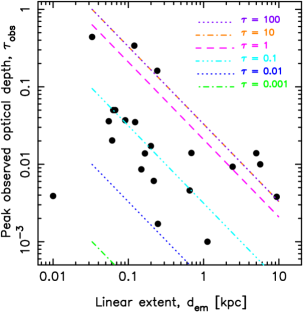
Figure 3: As Fig. 2, but for $f=d_{\rm abs}/d_{\rm em}$ and $d_{\rm abs}=33$ pc (the smallest of the bulk values of $d_{\rm em}$, i.e. excluding the outlier at $d_{\rm em}\approx 10$ pc). Again, the $\tau=10$ and $100$ lines are coincident.

This suggests that the geometry of the emission could be dominant along a single axis. This may be expected since high resolution imaging reveals the sources of emission to usually be two main lobes (e.g. Tzioumis et al. 2002; Pihlström et al. 2003 and references therein), with the extent of the radio emission being determined by the lobe separation. We now explore this, in conjunction with the possibility that the large range of emitter sizes may be due to projection effects, by extending the sample to also include the non-compact sources.

2.2 Extending to the general population of radio sources

In discussing the effects of radio source size on the strength of the 21-cm absorption, Curran & Whiting (2010) noted that the addition of non-compact/unclassified sources did not dilute the anti-correlation. Furthermore, from optical, near and far-infrared observations, no difference is found between compact and extended radio sources (de Vries et al. 1998 and Fanti et al. 2000, respectively). Including the non-compact/unclassified objects for which $d_{\rm em}$ is available (e.g. Gupta et al. 2006), the Kendall’s $\mathcal{T}$ two-sided probability of the correlation between observed optical depth and projected source size arising by chance is $P(\mathcal{T})=0.0044$. This is in comparison to the $P(\mathcal{T})<0.01$ “column density” correlation (Pihlström et al., 2003) and corresponds to a significance of $2.84\sigma$, assuming Gaussian statistics (Fig. 4).

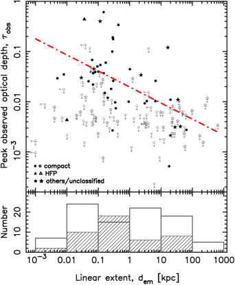
Figure 4: The peak observed optical depth versus the projected linear size (where available) for all of the redshifted radio sources searched in 21-cm absorption to date (compiled in Curran & Whiting 2010; Allison et al. 2012).The filled markers/hatched histogram represent the detections and the unfilled markers/histogram show the $3\sigma$ upper limits to the optical depth for the non-detections at a spectral resolution of 167 ${\rm km\ s}^{-1}$ (see Curran et al. 2013a). The circles designate compact objects and the stars non-compact/unclassified, with the triangles showing the high frequency peaker galaxies, which, although compact, Orienti et al. (2006) argue do not follow the trend. The line shows the least-squares-fit to the detections.

Gupta et al. (2006) state that the incidence of H i absorption is much higher for compact sources than for extended sources. The histogram in Fig. 4 shows the relative number of detections (hatched) and non-detections (unfilled) in each $\log_{10}(d_{\rm em})$ bin. One thing immediately obvious from this is that, while the detection rates are $\stackrel{{\scriptstyle<}}{{{}_{\sim}}}30$% in all other bins, between 0.1 and 1 kpc the rate exceeds 50%. A peak in the observed optical depth is also apparent in this bin (the top panel of Fig. 4). That is, there may exist a “resonance” between the absorber and radio source size. This could arise if when $d_{\rm abs}\ll d_{\rm em}$ the covering factor is low, whereas when $d_{\rm abs}\gg d_{\rm em}$, the chance of a misalignment between the absorber and emitter along our sight-line is greater for a smaller emission region, indicative of a clumpy absorbing medium. Interestingly, $\sim 100$ pc is the scale of the densest H i clouds found from low redshift emission studies (Braun, 2012).

We find the 21-cm detection rate to be 39% (30/77) at $d_{\rm em}<1$ kpc, in comparison to 23% (14/60) at $d_{\rm em}>1$ kpc, confirming a slightly higher detection rate for the compact sources. However, this is elevated by the 0.1 – 1 kpc bin. Furthermore, if the linear extent of the source is correlated with its luminosity, in conjunction with the fact that the radio and ultra-violet luminosities are correlated (Allison et al., 2012), we would expect a lower detection rate for the large/more luminous sources, due to ionisation of the gas by the active galactic nucleus (Curran & Whiting, 2012). When sources above the critical luminosity ($L_{\rm UV}\sim 10^{23}$ W Hz^-1) are removed, 21-cm detection rates in compact objects are not significantly higher than for the rest of the population (Curran & Whiting, 2010).

2.3 Absorption of a double lobed radio source

In order to test whether the wide range in observed source sizes could, at least in part, be caused by projection effects, we model the source size, $d_{\rm em}$, through the inclination, $i$, of a small range of intrinsic sizes. That is, $d_{\rm em}=t+d\cos i$, where $t$ is the diameter of the lobe and $d$ the deprojected space between the lobe centres (Fig. 5).

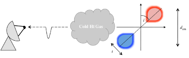
Figure 5: Schematic of the model showing projected linear size, $d_{\rm em}$ in relation to the lobe inclination, $i$, and thickness, $t$ (Glowacki, 2012).

As described by Glowacki (2012), the cross-sectional area of the lobes intercepted by a spherical absorber, i.e. the covering factor, was recorded when incrementing the inclination. Although there may be a preferred absorber size (Sect. 2.2), we do not know the underlying distribution of the intrinsic properties (such as optical depth and deprojected size) and so cannot perform a reliable statistical fit to these data. Therefore, for various intrinsic optical depths, $\tau$, the covering factor was converted to the observed optical depth via $\tau_{\rm obs}=f(1-e^{-\tau})$, with the best fit to the trend of the detections judged by eye. Different models were tested through the variation of several parameters:

• Varying the relative sizes of the model components: Specifically, the size of the absorber in relation to the lobe size, lobe thickness and spacing between the lobes, as well variation of the relative sizes between these three parameters. Generally, an absorber size close to or larger than the deprojected spacing between the lobes gave the better fit.

• Varying the lobe morphologies: Several morphologies were tested, with the best results being obtained by an ellipsoid, modelling the dominant jet morphology of an FRi source (Fanaroff & Riley, 1974), and a “lollipop”, modelling the faint jet plus hot-spot morphology of an FRii source.

• Introducing a non-uniform density distribution: In order to simulate the clumpy nature of the absorber, the points forming the density distribution were generated randomly, where if a value (RA_n,$\delta_{n}$) is at a radius smaller than the next generated value (RA_n+1,$\delta_{n+1}$), then absorption occurs at (RA_n,$\delta_{n}$). As seen from Fig. 6, this yields a clumpy distribution in which the density of absorbing points falls with radius. Using the non-uniform absorber has the effect of smoothing the dependence of the observed optical depth on inclination, generally providing a better match to the data than a uniformly dense absorber.

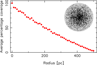
Figure 6: A single realisation of the average coverage with radius for a 1 kpc non-uniform absorber. The inset shows the density distribution in the RA–$\delta$ plane.

In Figs. 7 and 8 we show distributions obtained for the FRi and FRii approximations, respectively, intercepted by a non-uniformly dense absorber of total extent 1 kpc (Fig. 6), which yielded the $\tau_{\rm obs}-d_{\rm em}$ slopes that best traced the observed distribution (Glowacki, 2012).

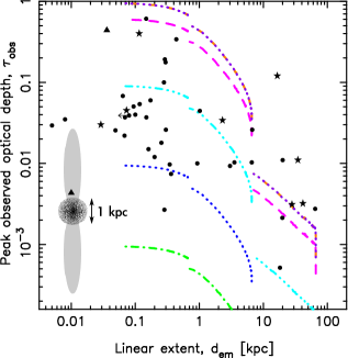
Figure 7: The observed optical depth versus the projected size (where available) for all of the 21-cm detections (see Fig. 4). The overlain lines show the variation for a non-uniformly dense absorber of $d_{\rm abs}=1$ kpc, occulting the elliptical lobe model (FRi), with $t=d/10$ for $d=0.66$, $6.6$ and $66$ kpc (the largest of the detections). The maximum value on the abscissa shows the deprojected size and on the ordinate the same values of $\tau_{\rm obs}$ as shown in Fig. 2. The inset illustrates the un-inclined 6.6 kpc model in the projected sky plane.

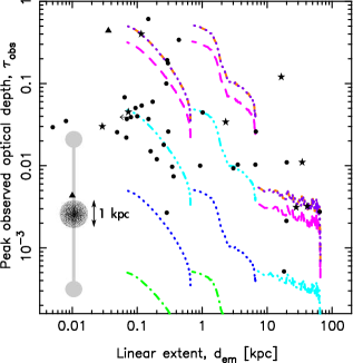
Figure 8: As Fig. 7, but for the lollipop model (FRii), again with a lobe diameter of $t=d/10$, for $d=0.66$, $6.6$ and $66$ kpc and a “stick” width $d/60$.

From these, just as for the intrinsic optical depths (Sect. 2.1), the projection of a single intrinsic source size cannot account for the whole distribution (as found for the compact objects by Fanti et al. 1990), although a range of sizes in conjunction with a range of optical depths does exhibit a similar slope to the $\tau_{\rm obs}-d_{\rm em}$ anti-correlation. At large linear extents, there are two non-compact objects which are located away from the model “fits”, although these did not form part of the original sample which led to the perceived anti-correlation (cf. Figs. 2 and 3).

Lastly, Pihlström et al. (2003) model the absorbing gas as both a spherical cloud and a disk, centered on the nucleus (the origin of the axes in Fig. 5). In the former case the model results will be the same as presented above, since, for a given absorber, the covering factor is solely dependent on the projected area of the lobes intercepted by the absorber. In the latter case, where the absorption is occuring in the pc-scale torus or the kpc-scale galactic disk, with a fixed orientation perpendicular to the jet axis, we may expect the power law drop as seen by Pihlström et al. (2003), although this would be with respect to the observed optical depth and not the column density (cf. Figs. 1 and 2). However, from the incidence of 21-cm detections in type-1 and type-2 active galactic nuclei, Curran et al. (2008) conclude that the bulk absorption occurs in the galactic disk, which must be randomly orientated with respect to the torus. This rules out applying a generic model of the jet inclination to a disk distribution, although we would generally expect the observed optical depth to decrease with decreasing inclination due to a reduction in the covering factor (Sect. 2.1).

3 Discussion and summary

Knowledge of the density of neutral gas in the distant Universe is crucial to our understanding of its contribution to the cosmic mass density (e.g. Curran 2010 and references therein) and its relation to the star formation history (e.g. Hopkins & Beacom 2006). Therefore, any dependence of the total column density of the neutral gas has profound consequences in the interpretation of this and, since Pihlström et al. (2003) noted the column density to be anti-correlated with size of the radio source illuminating the H i cloud, this relationship has been confirmed several times, although no clear physical explanation has ever been provided.

Upon dissecting the components which make up the estimate of the column density, we find, as Pihlström et al., the correlation to be between the observed optical depth and radio source size. The former quantity is directly proportional to the covering factor, in the optically thin regime, which is itself inversely proportional to the source size. Therefore, these quantities are not independent, with an observed optical depth–source size anti-correlation expected purely from the definition of $\tau_{\rm obs}$ alone. It is the assumption of a common spin temperature and covering factor for all of the sources, which leads to the $N_{\rm HI}-d_{\rm em}$ anti-correlation.

Extending the sample to include the non-compact objects, as found by de Vries et al. (1998); Fanti et al. (2000), we find no distinct difference between these and the compact sources, with the non-compact objects also following the $\tau_{\rm obs}-d_{\rm em}$ anti-correlation. Also, while the 21-cm detection rate may be higher in compact objects (e.g. Gupta et al. 2006), this could be dominated by a “resonance” at $d_{\rm em}\approx 0.1-1$ kpc, in addition to the fact that the larger sources may have higher ultra-violet luminosities, decreasing the likelihood of detecting neutral gas (Curran & Whiting, 2010). This resonance, where the 21-cm detection rate is significantly higher than for other values of $d_{\rm em}$, may indicate that the typical cross section of cold absorbing gas is of the order $100-1000$ pc.

Finally, through a model of a double lobed radio source, where the projected linear size, $d_{\rm em}$, depends upon the inclination, we find that the anti-correlation can be best accounted for models which approximate either of the two Fanaroff & Riley classifications and a non-uniformly dense absorber with a diameter in the range of the resonant $d_{\rm em}$. We also confirm the finding of Fanti et al. (1990) that the observed range in source extents cannot be accounted for by the inclination of a single deprojected size.

References

- Allison et al. (2012) Allison J. R. et al., 2012, MNRAS, 423, 2601
- Braun (2012) Braun R., 2012, ApJ, 87, 749
- Chandola et al. (2011) Chandola Y., Sirothia S. K., Saikia D. J., 2011, MNRAS, 418, 1787
- Curran (2010) Curran S. J., 2010, MNRAS, 402, 2657
- Curran (2012) Curran S. J., 2012, ApJ, 748, L18
- Curran et al. (2007) Curran S. J., Tzanavaris P., Pihlström Y. M., Webb J. K., 2007, MNRAS, 382, 1331
- Curran & Whiting (2010) Curran S. J., Whiting M. T., 2010, ApJ, 712, 303
- Curran & Whiting (2012) Curran S. J., Whiting M. T., 2012, ApJ, 759, 117
- Curran et al. (2011a) Curran S. J. et al., 2011a, MNRAS, 413, 1165
- Curran et al. (2013a) Curran S. J., Whiting M. T., Sadler E. M., Bignell C., 2013a, MNRAS, 428, 2053
- Curran et al. (2013b) Curran S. J., Whiting M. T., Tanna A., Sadler E. M., Athreya R., 2013b, MNRAS, 429, 3402
- Curran et al. (2011b) Curran S. J., Whiting M. T., Webb J. K., Athreya A., 2011b, MNRAS, 414, L26
- Curran et al. (2008) Curran S. J., Whiting M. T., Wiklind T., Webb J. K., Murphy M. T., Purcell C. R., 2008, MNRAS, 391, 765
- de Vries et al. (1998) de Vries W. H., O’Dea C. P., Perlman E., Baum S. A., Lehnert M. D., Stocke J., Rector T., Elston R., 1998, ApJ, 503, 138
- Fanaroff & Riley (1974) Fanaroff B. L., Riley J. M., 1974, MNRAS, 167, 31P
- Fanti (2000) Fanti C., 2000, in EVN Symposium 2000, Proceedings of the 5th european VLBI Network Symposium, Conway J. E., Polatidis A. G., Booth R. S., Pihlström Y. M., eds., p. 73
- Fanti et al. (1995) Fanti C., Fanti R., Dallacasa D., Schilizzi R. T., Spencer R. E., Stanghellini C., 1995, A&A, 302, 317
- Fanti et al. (2000) Fanti C. et al., 2000, A&A, 358, 499
- Fanti et al. (1990) Fanti R., Fanti C., Schilizzi R. T., Spencer R. E., Nan Rendong, Parma P., van Breugel W. J. M., Venturi T., 1990, A&A, 231, 333
- Glowacki (2012) Glowacki M., 2012, The Effects of Geometry on the Apparent Star-Forming Gas Abundance in Radio Galaxies. Tech. rep., University of Sydney
- Gupta & Saikia (2006a) Gupta N., Saikia D. J., 2006a, MNRAS, 370, L80
- Gupta & Saikia (2006b) Gupta N., Saikia D. J., 2006b, MNRAS, 370, 738
- Gupta et al. (2006) Gupta N., Salter C. J., Saikia D. J., Ghosh T., Jeyakumar S., 2006, MNRAS, 373, 972
- Gupta et al. (2012) Gupta N., Srianand R., Petitjean P., Bergeron J., Noterdaeme P., Muzahid S., 2012, A&A, 544, 21
- Hopkins & Beacom (2006) Hopkins A. M., Beacom J. F., 2006, ApJ, 651, 142
- Kanekar & Chengalur (2003) Kanekar N., Chengalur J. N., 2003, A&A, 399, 857
- Lavalley et al. (1992) Lavalley M. P., Isobe T., Feigelson E. D., 1992, in BAAS, Vol. 24, pp. 839–840
- O’Dea (1998) O’Dea C. P., 1998, PASP, 110, 493
- O’Dea et al. (1994) O’Dea C. P., Baum S. A., Gallimore J. F., 1994, ApJ, 436, 669
- Orienti et al. (2006) Orienti M., Morganti R., Dallacasa D., 2006, A&A, 457, 531
- Pihlström et al. (2003) Pihlström Y. M., Conway J. E., Vermeulen R. C., 2003, A&A, 404, 871
- Tzioumis et al. (2002) Tzioumis A. et al., 2002, A&A, 392, 841
- van Breugel et al. (1984) van Breugel W., Miley G., Heckman T., 1984, AJ, 89, 5
- Wolfe & Burbidge (1975) Wolfe A. M., Burbidge G. R., 1975, ApJ, 200, 548