Grating monochromator for soft X-ray self-seeding the European XFEL

Abstract

Self-seeding is a promising approach to significantly narrow the SASE bandwidth of XFELs to produce nearly transform-limited pulses. The implementation of this method in the soft X-ray wavelength range necessarily involves gratings as dispersive elements. We study a very compact self-seeding scheme with a grating monochromator originally designed at SLAC, which can be straightforwardly installed in the SASE3 type undulator beamline at the European XFEL. The monochromator design is based on a toroidal VLS grating working at a fixed incidence angle mounting without entrance slit. It covers the spectral range from $300$ eV to $1000$ eV. The optical system was studied using wave optics method (in comparison with ray tracing) to evaluate the performance of the self-seeding scheme. Our wave optics analysis takes into account the actual beam wavefront of the radiation from the coherent FEL source, third order aberrations, and errors from each optical element. Wave optics is the only method available, in combination with FEL simulations, for the design of a self-seeding monochromator without exit slit. We show that, without exit slit, the self-seeding scheme is distinguished by the much needed experimental simplicity, and can practically give the same resolving power (about 7000) as with an exit slit. Wave optics is also naturally applicable to calculations of the self-seeding scheme efficiency, which include the monochromator transmittance and the effect of the mismatching between seed beam and electron beam. Simulations show that the FEL power reaches $1$ TW and that the spectral density for a TW pulse is about two orders of magnitude higher than that for the SASE pulse at saturation.

DEUTSCHES ELEKTRONEN-SYNCHROTRON

Ein Forschungszentrum der Helmholtz-Gemeinschaft

DESY 13-040

March 2013

Grating monochromator for soft X-ray self-seeding the European XFEL

Svitozar Serkez^a, Gianluca Geloni^b, Vitali Kocharyan^a and Evgeni Saldin^a

^aDeutsches Elektronen-Synchrotron DESY, Hamburg

^bEuropean XFEL GmbH, Hamburg ISSN 0418-9833 NOTKESTRASSE 85 - 22607 HAMBURG

1 Introduction

Self-seeding is a promising approach to significantly narrow the SASE bandwidth and to produce nearly transform-limited pulses SELF -OURY5b . Considerable effort has been invested in theoretical investigation and $R\&D$ at the LCLS leading to the implementation of a hard X-ray self-seeding (HXRSS) setup that relies on a diamond monochromator in transmission geometry. Following the successful demonstration of the HXRSS setup at the LCLS EMNAT , there is a need for an extension of the method in the soft X-ray range.

In general, a self-seeding setup consists of two undulators separated by a photon monochromator and an electron bypass, normally a four-dipole chicane. The two undulators are resonant at the same radiation wavelength. The SASE radiation generated by the first undulator passes through the narrow-band monochromator. A transform-limited pulse is created, which is used as a coherent seed in the second undulator. Chromatic dispersion effect in the bypass chicane smears out the microbunching in the electron bunch produced by the SASE lasing in the first undulator. The electrons and the monochromatized photon beam are recombined at the entrance of the second undulator, and radiation is amplified by the electron bunch until saturation is reached. The required seed power at the beginning of the second undulator must dominate over the shot noise power within the gain bandpass, which is order of a kW in the soft X-ray range.

For self-seeding in the soft x-ray range, proposed monochromators usually consists of a grating SELF , STTF . Recently, a very compact soft x-ray self-seeding (SXRSS) scheme has appeared, based on grating monochromator FENG -FENG3 . The delay of the photons in the last SXRSS version FENG3 is about $0.7$ ps only. The proposed monochromator is composed of only three mirrors and a toroidal VLS grating. The design adopts a constant, $1$ degree incidence-angle mode of operation, in order to suppress the influence of movement of the source point in the first SASE undulator on the monochromator performance.

In this article we study the performance of the soft X-ray self-seeding scheme for the European XFEL upgrade. In order to preserve the performance of the baseline undulator, we fit the magnetic chicane within the space of a single $5$ m undulator segment space at SASE3. In this way, the setup does not perturb the undulator focusing system. The magnetic chicane accomplishes three tasks by itself. It creates an offset for monochromator installation, it removes the electron microbunching produced in the upstream seed undulator, and it acts as an electron beam delay line for compensating the optical delay introduced by the monochromator. The monochromator design is compact enough to fit with this magnetic chicane design. The monochromator design adopted in this paper is an adaptation of the novel one by Y. Feng et al. FENG3 , and is based on toroidal VLS grating, and has many advantages. It consists of a few elements. In particular, it operates without entrance slit, and is, therefore, very compact. Moreover, it can be simplified further. Quite surprisingly, a monochromatic seed can be directly selected by the electron beam at the entrance of the second undulator. In other words, the electron beam plays, in this case, the role of an exit slit. By using a wave optics approach and FEL simulations we show that the monochromator design without exit slits works in a satisfactory way.

With the radiation beam monochromatized down to the Fourier transform limit, a variety of very different techniques leading to further improvement of the X-ray FEL performance become feasible. In particular, the most promising way to extract more FEL power than that at saturation is by tapering the magnetic field of the undulator TAP1 -WANG . A significant increase in power is achievable by starting the FEL process from a monochromatic seed rather than from shot noise FAWL -LAST . In this paper we propose a study of the soft X-ray self-seeding scheme for the European XFEL, based on start-to-end simulations for an electron beam with 0.1 nC charge S2ER . Simulations show that the FEL power of the transform-limited soft X-ray pulses may be increased up to 1 TW by properly tapering the baseline (SASE3) undulator. In particular, it is possible to create a source capable of delivering fully-coherent, 10 fs (FWHM) soft X-ray pulses with $10^{14}$ photons per pulse in the water window.

The availability of free undulator tunnels at the European XFEL facility offers a unique opportunity to build a beamline optimized for coherent diffraction imaging of complex molecules like proteins and other biologically interesting structures. Full exploitation of these techniques require 2 keV - 6 keV photon energy range and TW peak power pulses. However, higher photon energies are needed to reach anomalous edges of commonly used elements (such as Se) for anomalous experimental phasing. Potential users of the bio-imaging beamline also wish to investigate large biological structures in the soft X-ray photon energy range down to the water window. A conceptual design for the undulator system of such a bio-imaging beamline based on self-seeding schemes developed for the European XFEL was suggested in BIO1 -BIO3 . The bio-imaging beamline would be equipped with two different self-seeding setups, one providing monochromatization in the hard x-ray wavelength range, using diamond monochromators and one providing monochromatization in the soft x-ray range using a grating monochromator. In relation to this proposal, we note that the design for a soft x-ray self-seeding scheme discussed here can be implemented not only at the SASE3 beamline but, as discussed in BIO1 -BIO3 , constitutes a suitable solution for the bio-imaging beamline in the soft x-ray range as well.

2 Self-seeding setup description

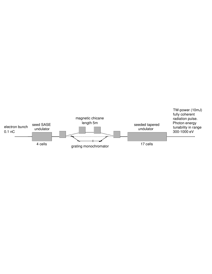
Figure 1: Design of the SASE3 undulator system for TW mode of operation in the soft X-ray range.

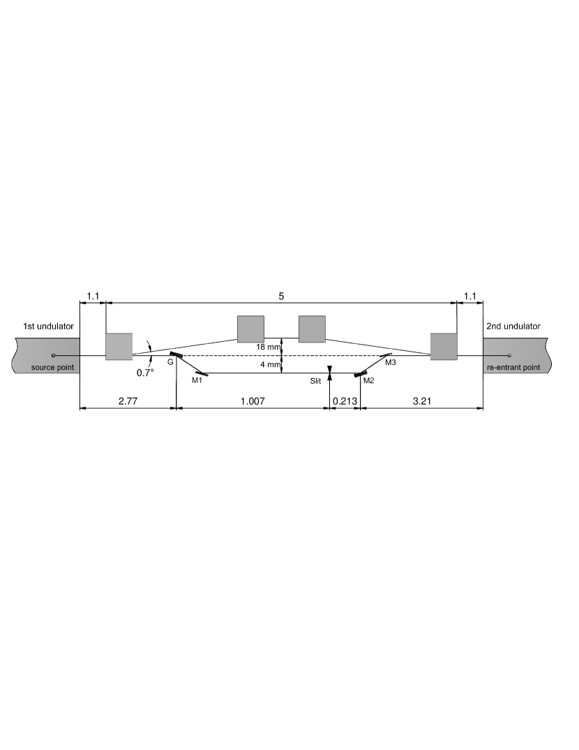
Figure 2: Layout of the SASE3 self-seeding system, to be located in the space freed after removing the undulator segment U5. The compact grating monochromator design relies on a scheme originally proposed at SLAC. G is a toroidal VLS grating. M1 is a rotating plane mirror, M2 is a tangential cylindrical mirror, M3 is a plane mirror used to steer the beam. The deflection of both electron and photon beams is in the horizontal direction.

Figure 3: Focusing at the slit. Distance between waist, characterized by plane wavefront, and grating as a function of the photon energy.

Figure 4: Focusing at the slit. Variation of the distance between waist and slit normalized on the Rayleigh range as a function of the photon energy.

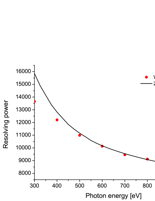
Figure 5: Resolving power as a function of the photon energy for a monochromator equipped with exit slit (bold curve) and without exit slit (circles). The calculation with exit slit is for a slit width of $2\mu$m.

Figure 6: Current profile for a $100$ pC electron bunch at the entrance of the first undulator.

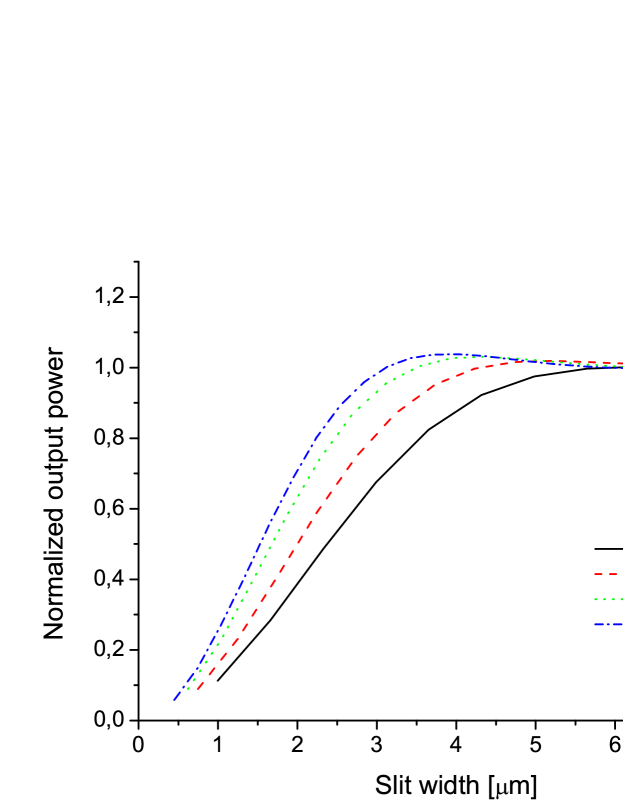
Figure 7: Results of seeding efficiency simulations, showing the normalized output power from the second FEL amplifier as a function of the exit slit width for different photon energies. The FEL amplifier operates in the linear regime. Results are obtained by wave optics and FEL simulations.

Figure 8: First order efficiency of the blazed groove profile. Here the groove density is $1100$ lines/mm, Pt coating is assumed, at an incidence angle of $1^{\circ}$. The blaze angle is $1.2^{\circ}$; the anti-blaze angle is $90^{\circ}$.

Figure 9: Power distribution and spectrum of the SASE soft x-ray radiation pulse at the exit of the first undulator.

Figure 10: Line profile of the self-seeding monochromator without exit slit. The calculation is for a photon energy of $0.8$ keV. The overall efficiency of the monochromator beamline is about $5\%$.

Figure 11: Power distribution and spectrum of the SASE soft x-ray radiation pulse after the monochromator. This pulse is used to seed the electron bunch at the entrance of the second undulator.

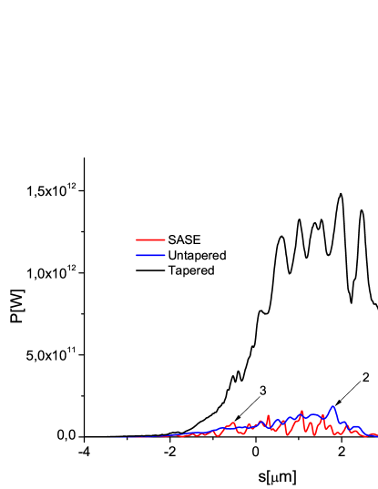
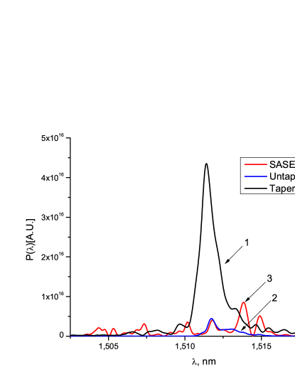
Figure 12: Power distribution and spectrum of the output soft x-ray radiation pulse. Curve 1 - seeded FEL output with tapering; curve 2 - seeded FEL output without tapering; curve 3 - SASE FEL output in saturation. Here $\lambda=1.5$ nm, corresponding to $800$ eV.

Figure 13: Energy of the seeded FEL pulse as a function of the distance inside the output undulator.

Table 1: Parameters for the x-ray optical elements
¹ Distance to grating.
² Principal ray hit point.

Element	Parameter	Value at photon energy			Required precision	Unit
		300 eV	600 eV	1000 eV
G	Line density ($k$)	1123			0.2%	l/mm
G	Linear coeff ($n_{1}$)	2.14			1%	l/mm2
G	Quad coeff ($n_{2}$)	0.003			50%	l/mm3
G	Groove profile	Blased 1.2∘			-	-
G,M1	Roughness (rms)	-			2	nm
G	Tangential radius	160			1%	m
G	Sagittal radius	0.25			10%	m
G	Diffraction order	+1				-
G	Incident angle	1			-	deg
G	Exit angle	5.615	4.028	3.816	-	deg
	Source distance	3160	3470	3870	-	mm
	Source size	30.3	27.7	24.2	-	$\mu$m
	Image distance	1007	1004	1007	-	mm
	Image size	2.22	2.45	2.22	-	$\mu$m
M1	Location	33.2	43.8	52.6	-	mm
M1	Incident angle	3.307	2.514	2.093	-	deg
S	Slit location	1007			0.5	mm
S	Slit width	2			5%	$\mu$m
M2	Location	1220			1	mm
M2	Incident angle	0.859			-	deg
M2	Tangential radius	27.3			1%	m
M3	Location	1348.3			-	mm
M3	Incident angle	0.859			-	deg
	Optical delay	935	757	662	-	fs

A design of the self-seeding setup based on the undulator system for the European XFEL baseline is sketched in Fig. 1. The method for generating highly monochromatic, high power soft x-ray pulses exploits a combination of a self-seeding scheme with grating monochromator with an undulator tapering technique. The self-seeding setup is composed by a compact grating monochromator originally proposed at SLAC FENG3 , yielding about $0.7$ ps optical delay, and a $5$ m-long magnetic chicane.

Usually, a grating monochromator consists of an entrance slit, a grating, and an exit slit. The grating equation, which describes how the monochromator works, relies on the principle of interference applied to the light coming from the illuminated grooves. Such principle though, can only be applied when phase and amplitude variations in the electromagnetic field are well-defined across the grating, that is when the field is perfectly transversely coherent. The purpose of the entrance slit is to supply a transversely coherent radiation spot at the grating, in order to allow the monochromator to work with an incoherent source and with a given resolution. However, an FEL source is highly transversely coherent and no entrance slit is required in this case SVET , ROPE .

Fig. 2 shows the optical configuration of the self-seeding monochromator. Table 1 summarizes the optical parameters of the setup. The design of the monochromator was optimized with respect to the resolving power and the seeding efficiency. The design energy range of the monochromator is in the $0.3$ keV - $1$ keV interval with a resolution of about $7000$. It is only equipped with an exit slit. A toroidal grating with variable line spacing (VLS) is used for imaging the FEL source to the exit slit of the monochromator. The grating has a groove density of $1120$ lines/mm. The first coefficient $D_{1}$ of the VLS grating is $D_{1}=2.1/\mathrm{mm}^{2}$. The grating will operate in fixed incident angle mode in the $+1$ order. The incident X-ray beam is imaged at the exit slit and re-imaged at the entrance of the seed undulator by a cylindrical mirror M2. In the sagittal plane, the source is imaged at the entrance of the seed undulator directly by the grating. The monochromator scanning is performed by rotating the post-grating plane mirror. The scanning results on a wavelength-dependent optical path. Therefore, a tunability of the path length in the magnetic chicane in the range of $0.05$ mm is required to compensate for the change in the optical path.

The choice was made to use a toroidal VLS grating similar to the LCLS design FENG3 . As pointed out in that reference, the source point in the SASE undulator moves upstream with the photon energy. The proposed design has been chosen in order to minimize the variation of the image distance. The object distance was based on FEL simulations of the SASE3 undulator at the exit of the fourth segment U4, Fig. 1. The monochromator performance was calculated using wave optics. The exact location of the waist, characterized by a plane wavefront, Fig. 3 and Fig. 4, was found to vary with the energy around the slit within $2.7$ mm, which is small compared to the Rayleigh range, Fig. 4. This defocusing effect was fully accounted for in the wave optics treatment, and the impact of this effect on the resolving power is negligible. The resolving power achievable with the exit slit is shown in Fig. 5. It approaches $8000$, and is sufficient to produce temporally transform-limited seed pulses with FWHM duration between $25$ fs and $50$ fs over the designed photon energy range. This duration is sufficiently longer than the FWHM duration of the electron bunch, about $15$ fs in standard mode of operation at $0.1$ nC charge, Fig. 6. The resolving power depends on the size of the FEL source inside the SASE undulator, on the size of the exit slit (assumed fixed at $2\mu$m) and on third order optical aberrations.

The operation of the self-seeding scheme involves simultaneous presence of monochromatized radiation and electron beam in the seed undulator. This suggests to consider a particularly interesting approach to solve the task of creating a monochromatized seed. In fact, the resolving power needed for seeding can be achieved without exit slit by combining the presence of radiation and electron beam in the seed undulator. The influence of the spatial dispersion in the image plane at the entrance of the seed undulator on the operation of the self-seeding setup without exit slit can be quantified by studying the input coupling factor between the seed beam and the ground mode of the FEL amplifier. A combination of wave optics and FEL simulations is the only method available for designing such self-seeding monochromator without exit slit. This design has the advantage of a much needed experimental simplicity, and could deliver a resolving power as that with the exit slit. The comparison of resolving powers for these two designs is shown in Fig. 5. The size of the beam waist near the slit is about $2.2$-$2.4~{}\mu$m. The operation without exit slit would give worse resolving power than the conventional mode of operation only when the slit size is smaller than $2~{}\mu$m. Wave optics and FEL simulations are naturally applicable also for calculating suppression of the input coupling factor, due to the effect of a finite size of the exit slit. The effect of the slit on the seeding efficiency shown in Fig. 7. When the slit size is smaller than $2~{}\mu$m, the effective seed power is reduced by as much as a factor $2-3$. We conclude that the mode of operation without exit slit is superior to the conventional mode of operation, and a finite slit size would only lead to a reduction of the monochromator performance.

The efficiency of the grating should be specified over the range of photon energies where the grating will be used. The efficiency was optimized by varying the groove shapes. Blazed grating was optimized by adjusting the blaze angle; sinusoidal grating by adjusting the groove depth, and rectangular grating by adjusting the groove depth, and assuming a duty cycle of $50\%$. The blazed profile is substantially superior to both sinusoidal and laminar alternatives. For the specified operating photon energy range, the optimal blaze angle is $1.2$ degree, and the expected grating efficiency with platinum coating is shown in Fig. 8. This curve assumes a constant incident angle of $1$ degree.

The electron beam chicane contains four identical dipole magnets, each of them $0.5$ m-long. Given a magnetic field $B=0.8T$ and an electron momentum $p=10$GeV/c, this length corresponds to a dipole bending angle of $0.7$ degrees. The choice of the strength of the magnetic chicane only depends on the delay that we want to introduce. In our case, as already mentioned, it amounts to $0.23$ mm, or $0.7$ ps. Parameters discussed above fit with a short, $5$ m-long magnetic chicane to be installed in place of a single undulator module. Such chicane, albeit very compact, is however strong enough to create a sufficiently large transverse offset for the installation of the optical elements of the monochromator.

Despite the unprecedented increase in peak power of the X-ray pulses at SASE X-ray FELs some applications, including bio-imaging , require still higher photon flux HAJD -BERG . The most promising way to extract more FEL power than that at saturation is by tapering the magnetic field of the undulator. Tapering consists in a slow reduction of the field strength of the undulator in order to preserve the resonance wavelength, while the kinetic energy of the electrons decreases due to FEL process. The undulator taper could be simply implemented at discrete steps from one undulator segment to the next. The magnetic field tapering is provided by changing the undulator gap. Here we study a scheme for generating TW-level soft X-ray pulses in a SASE3 tapered undulator, taking advantage of the highly monochromatic pulses generated with the self-seeding technique, which make the tapering very efficient. We optimized our setup based on start-to-end simulations for an electron beam with $100$ pC charge. In this way, the output power of SASE3 could be increased from the baseline value of $100$ GW to about a TW in the photon energy range between $0.3$ keV and $1$ keV.

Summing up, the overall self-seeding setup proposed here consists of three parts: a SASE undulator, a self-seeding grating monochromator and an output undulator in which the monochromtic seed signal is amplified up to the TW power level. Calculations show that in order not to spoil the electron beam quality and to simultaneously reach signal dominance over shot noise, the number of cells in the first (SASE) undulator should be equal to $4$. The output undulator consists of two sections. The first section is composed by an uniform undulator, the second section by a tapered undulator. The transform-limited seed pulse is exponentially amplified passing through the first uniform part of the output undulator. This section is long enough, $6$ cells, in order to reach saturation, which yields about $100$ GW power. Finally, in the second part of the output undulator the monochromatic FEL output is enhanced up to the TW power level taking advantage of a $3.5\%$ taper of the undulator magnetic field over the last $11$ cells after saturation.

Simulations were performed with the help of the Genesis code GENE running on a cluster in the following way: first we calculated the 3D field distribution at the exit of the first undulator, and downloaded the field file. Subsequently, we performed a temporal Fourier transformation followed by filtering through the monochromator, by using the filter amplitude transfer function. The electron microbunching is washed out by presence of non-zero chicane momentum compaction factor $R_{56}$. Therefore, for the second undulator we used a beam file with no initial microbunching, and with an energy spread induced by the FEL amplification process in the first SASE undulator. The amplification process in the second undulator starts from the seed field-file. Shot noise initial conditions were included, see section 5 for details. The output power and spectrum after the first (SASE) undulator tuned at $1.5$ nm is shown in Fig. 9. The instrumental function is shown in Fig. 10. The shape of this curve was found as a response of the input coupling factor on the offset of the seed monochromatic beam at the entrance of the seed undulator due to spatial dispersion. The absolute value of the transmittance accounts for the absorption of the monochromatic beam in the grating and in the three mirrors, for a total of $5\%$. The influence of the transverse mismatching of the seed beam at the entrance of the seed undulator is accounted for by an additional suppression of the input coupling factor. The resolution of the self-seeding monochromator is good enough, and the spectral width of the filter is a few times shorter than the coherent spectral interval (usually referred to as ”spike”) in the SASE spectrum. Therefore, the seed radiation pulse is temporally stretched in such way that the final shape only depends on the characteristics of the monochromator. The temporal shape and spectrum of the seed signal are shown in Fig. 11. The overall duration of the seed pulse is inversely proportional to the bandwidth of the monochromator transmittance spectrum. The particular temporal shape of the seed pulse simply follows from a Fourier transformation of the monochromator transfer function. The output FEL power and spectrum of the entire setup, that is after the second part of the output undulator is shown in Fig. 12. The evolution of the output energy in the photon pulse as a function of the distance inside the output undulator is reported in Fig. 13. The photon spectral density for a TW pulse is about two orders of magnitude higher than that for the SASE pulse at saturation (see Fig. 12). Given the fact that the TW-pulse FWHM-duration is about $10$ fs, the relative bandwidth is 3 times wider than the transform-limited bandwidth. There is a relatively large energy chirp in the electron bunch due to wakefields effect. Nonlinear energy chirp in the electron bunch induces nonlinear phase chirp in the seed pulse during the amplification process in the output undulator. Our simulations automatically include this effect. This phase chirp increases the time-bandwidth product by broadening the seeded FEL spectrum (see section 5 for details).

3 Theoretical background for designing a grating monochromator

3.1 Wave optics approach

In this section we derive the spatial frequency transfer function for wave propagation and the Fresnel diffraction formula commonly used in Fourier optics. We then analyze the propagation of a Gaussian beam through ideal lenses and mirrors spaced apart from each other.

3.1.1 Spatial frequency transfer function and spatial impulse response for wave propagation

We start from the homogeneous wave equation for the electric field in the space-time domain, $\vec{E}(t,\vec{r})$ expressed in cartesian coordinates:

$$\nabla^{2}\vec{E}-\frac{1}{c^{2}}\frac{\partial^{2}\vec{E}}{\partial t^{2}}=0~{}.$$ (3)

Here $c$ indicates the speed of light in vacuum, $t$ is the time and $\vec{r}$ is a 3D spatial vector identified by cartesian coordinates $x,y,z$. As a consequence, the following equation for the field $\vec{\bar{E}}(\omega,\vec{r})$ in the space-frequency domain holds:

$$\nabla^{2}\vec{\bar{E}}+k_{0}^{2}\vec{\bar{E}}=0~{},$$ (4)

where $k_{0}=\omega/c$. Eq. (4) is the well-known Helmholtz equation. Here $\vec{\bar{E}}(\omega,\vec{r})$ is temporal Fourier transform of the electric field. We explicitly write the definitions of the Fourier transform and inverse Fourier transform for a function $f(t)$ in agreement with the notations used in this paper as:

$$\bar{f}(\omega)=\int_{-\infty}^{\infty}f(t)\exp[i\omega t]dt~{}~{},$$ (5)

$$f(t)=\frac{1}{2\pi}\int_{-\infty}^{\infty}\bar{f}(\omega)\exp[-i\omega t]d\omega$$ (6)

Similarly, the 2D spatial Fourier transform of $\vec{\bar{E}}(x,y,z,\omega)$, with respect to the two transverse coordinates $x$ and $y$ will be written as

$$\vec{\hat{E}}(\omega,k_{x},k_{y},z)=\int_{-\infty}^{\infty}dx\int_{-\infty}^{\infty}dy\vec{\bar{E}}(\omega,x,y)\exp[ik_{x}x+ik_{y}y]~{},$$ (7)

so that

$$\vec{\bar{E}}(\omega,x,y,z)=\frac{1}{4\pi^{2}}\int_{-\infty}^{\infty}dk_{x}\int_{-\infty}^{\infty}dk_{y}\vec{\hat{E}}(\omega,k_{x},k_{y})\exp[-ik_{x}x-ik_{y}y]~{}.$$ (8)

With the help of this transformation the Helmholtz equation, which is a partial differential equation in three dimensions, reduces to a one-dimensional ordinary differential equation for the spectral amplitude $\vec{\hat{E}}(\omega,k_{x},k_{y},z)$. In fact, by taking the 2D Fourier transform of Eq. (4), we have

$$\frac{d^{2}\vec{\hat{E}}}{dz^{2}}+k_{0}^{2}\left(1-\frac{k_{x}^{2}}{k_{0}}-\frac{k_{y}^{2}}{k_{0}^{2}}\right)\vec{\hat{E}}=0~{}.$$ (9)

We then obtain straightforwardly

$$\vec{\hat{E}}(\omega,k_{x},k_{y},z)=\vec{\hat{E}}(\omega,k_{x},k_{y},0)\exp\left[ik_{0}z\sqrt{1-\frac{k_{x}^{2}}{k_{0}^{2}}-\frac{k_{y}^{2}}{k_{0}^{2}}}\right]~{},$$ (10)

where $\hat{E}(\omega,k_{x},k_{y},z)$ is the output field and $\hat{E}(\omega,k_{x},k_{y},0)$ is the input field. Further on, when the temporal frequency $\omega$ will be fixed, we will not always include it into the argument of the field amplitude and simply write e.g. $\hat{E}(k_{x},k_{y},z)$. It is natural to define the spatial frequency response of the system as

$$H(k_{x},k_{y},z)=\frac{\vec{\hat{E}}(k_{x},k_{y},z)}{\vec{\hat{E}}(k_{x},k_{y},0)}=\exp\left[ik_{0}z\sqrt{1-\frac{k_{x}^{2}}{k_{0}^{2}}-\frac{k_{y}^{2}}{k_{0}^{2}}}\right]~{}.$$ (11)

Here the ratio between vectors has to be interpreted component by component. $H$ is the spatial frequency transfer function related with light propagation through a distance $z$ in free space. If we assume that $k_{x}^{2}+k_{y}^{2}\ll k_{0}^{2}$, meaning that the bandwidth of the angular spectrum of the beam is small we have

$$H(k_{x},k_{y},z)\simeq\exp[ik_{0}z]\exp\left[-\frac{iz}{2k_{0}}(k_{x}^{2}+k_{y}^{2})\right]~{}.$$ (12)

In other words, we enforce the paraxial approximation. In order to obtain the output field distribution in the space-frequency domain $\vec{\bar{E}}(x,y,z)$ at the distance z away from the input position at $z=0$, we simply take the inverse Fourier transform of Eq. (10). If the paraxial approximation is now enforced we obtain

$$\vec{\bar{E}}(x,y,z) =\int_{-\infty}^{\infty}\int_{-\infty}^{\infty}dx^{\prime}~{}dy^{\prime}~{}\vec{\bar{E}}(x^{\prime},y^{\prime},0)h(x-x^{\prime},y-y^{\prime},z)$$ (14)

$$=\vec{\bar{E}}(x,y,0)\ast h(x,y,z)~{},$$

where

$$h(x,y,z) =\frac{1}{4\pi^{2}}\exp[ik_{0}z]$$ (16)

$$\times\int_{-\infty}^{\infty}\int_{-\infty}^{\infty}dk_{x}~{}dk_{y}~{}\exp\left[-\frac{iz}{2k_{0}}(k_{x}^{2}+k_{y}^{2})\right]\exp[-ik_{x}x-ik_{y}y]~{}.$$

The result in Eq. (14) indicates that $h(x,y,z)$ is the spatial impulse response describing the propagation of the system in the formalism of Fourier optics. $h(x,y,z)$ is readily evaluated as

$$h(x,y,z)=-\frac{ik_{0}}{2\pi z}\exp[ik_{0}z]\exp\left[\frac{ik_{0}}{2z}(x^{2}+y^{2})\right]~{}.$$ (17)

Eq. (14) is the Fresnel diffraction formula. In order to obtain the output field distribution $\vec{\bar{E}}(x,y,z)$, we need to convolve the input field distribution $\vec{\bar{E}}(x,y,0)$ with the spatial impulse response $h(x,y,z)$.

3.1.2 Gaussian beam optics

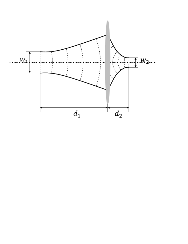
Figure 14: Gaussian beam transformation by a lens. A Gaussian beam with plane wavefront and waist $w_{1}$, located at a distance $d_{1}$ from the thin lens with focal length $f$ is transformed to a Gaussian beam of plane wavefront and waist $w_{2}$, located at a distance $d_{2}$, according to Eq. (38).

We now specialize our discussion considering a Gaussian beam with initially (at $z=0$) plane wavefront in two transverse dimensions. In order to simplify the notation, we will consider one component of the field in the space-frequency domain only.

$$\bar{E}(x,y,0)=A\exp\left[-\frac{x^{2}+y^{2}}{w_{0}^{2}}\right]~{},$$ (18)

where $w_{0}$ is the waist of the Gaussian beam. The spatial Fourier transform of $\bar{E}$ is given by

$$\hat{E}(k_{x},k_{y},0)=A\pi w_{0}^{2}\exp\left[-\frac{w_{0}^{2}}{4}\left(k_{x}^{2}+k_{y}^{2}\right)\right]~{}.$$ (19)

Using Eq. (12), after propagation over a distance $z$ one obtains

$$\hat{E}(k_{x},k_{y},z) =\hat{E}(k_{x},k_{y},0)H(k_{x},k_{y},z)$$ (22)

$$=A\pi w_{0}^{2}\exp[ik_{0}z]\exp\left[-\frac{iz}{2k_{0}}\left(k_{x}^{2}+k_{y}^{2}\right)\right]\exp\left[-\frac{w_{0}^{2}}{4}\left(k_{x}^{2}+k_{y}^{2}\right)\right]$$

$$=A\pi w_{0}^{2}\exp[ik_{0}z]\exp\left[-\frac{iq}{2k_{0}}(k_{x}^{2}+k_{y}^{2})\right]~{},$$

where $q$ is the so-called $q$-parameter of the Gaussian beam

$$q=z-iz_{R}~{},$$ (23)

where $z_{R}$ defines the Rayleigh range of the Gaussian beam

$$z_{R}=k_{0}w_{0}^{2}/2~{}.$$ (24)

The spatial profile of the beam after propagation through a distance $z$ can be found by taking the inverse Fourier transform of Eq. (22):

$$\bar{E}(x,y,z)=-\frac{iAk_{0}w_{0}^{2}}{2q}\exp[ik_{0}z]\exp\left[i\frac{k_{0}}{2q}(x^{2}+y^{2})\right]~{},$$ (25)

which can also be written as

$$\bar{E}(x,y,z) =A\frac{w_{0}}{w(z)}\exp[i\phi(z)+ik_{0}z]$$ (27)

$$\times\exp\left[-\frac{(x^{2}+y^{2})}{w^{2}(z)}\right]\exp\left[i\frac{k_{0}}{2R(z)}(x^{2}+y^{2})\right]~{},$$

where

$$w^{2}(z)=w_{0}^{2}\left[1+\left(\frac{z}{z_{R}}\right)^{2}\right]~{},$$ (28)

$$R(z)=\frac{1}{z}\left(z^{2}+z_{R}^{2}\right)~{},$$ (29)

and

$$\phi(z)=-\arctan\left[\frac{z}{z_{R}}\right]~{},$$ (30)

with $z_{R}$ defined in Eq. (24). Note that the width $w(z)$ of the Gaussian beam is a monotonically increasing function of the propagation distance $z$, and reaches $\sqrt{2}$ times its original width, $w_{0}$, at $z=z_{R}$. The radius of curvature $R(z)$ of the wavefront is initially infinite, corresponding to an initially plane wavefront, but it reaches a minimum value of $2z_{R}$ at $z=z_{R}$, before starting to increase again. The slowly varying phase $\phi(z)$, monotonically varies from $0$ at $z=0$ to $-\pi/2$ as $z\longrightarrow\infty$, assuming the value $\pi/4$ at $z=z_{R}$.

Note that the $q$-parameter contains all information about the Gaussian, namely its curvature $R(z)$ and its waist $w(z)$. The knowledge of the transformation of $q$ as a function of $z$ fully characterizes the behavior of the Gaussian beam.

An optical system would usually comprise lenses or mirrors spaced apart from each other. While Gaussian beam propagation in between optical elements can be tracked using the translation law above, Eq. (25), we still need to discuss the law for the transformation of $q$ by a lens. The transparency function for a thin converging lens is of the form

$$T_{f}(x,y)=\exp\left[-\frac{ik_{0}}{2f}(x^{2}+y^{2})\right]~{}.$$ (31)

The optical field immediately behind a thin lens at position $z$ is related to that immediately before a lens by

$$\bar{E}(x,y,z) =T_{f}(x,y)\bar{E}_{\mathrm{before}}(x,y,z)$$ (34)

$$=-\frac{iAk_{0}w_{0}^{2}}{2q}\exp[ik_{0}z]\exp\left[i\frac{k_{0}}{2q}(x^{2}+y^{2})\right]\exp\left[-\frac{ik_{0}}{2f}(x^{2}+y^{2})\right]$$

$$=-\frac{iAk_{0}w_{0}^{2}}{2q}\exp[ik_{0}z]\exp\left[i\frac{k_{0}}{2q_{l}}(x^{2}+y^{2})\right]$$

where $\bar{E}_{\mathrm{before}}(x,y,z)$ is given by Eq. (22) and $q_{l}$, the transformed of $q$, is defined by

$$\frac{1}{q_{l}}=\frac{1}{q}-\frac{1}{f}~{}.$$ (35)

As example of application we analyze the focusing of a Gaussian beam by a converging lens. We assume that a Gaussian beam with plane wavefront and waist $w_{1}$, is located at distance $d_{1}$ from a thin lens with focal length $f$. After propagation through a distance $d_{2}$ behind the lens, it is transformed to a beam with plane wavefront and waist $w_{2}$, Fig. 15. Using Eq. (23) and Eq. (35) we can find the transformed $q$-parameter at distance $d_{2}$. From Eq. (23), immediately in front of the lens we have

$$q(d_{1})=q(0)+d_{1}~{},$$ (36)

Immediately behind the lens, the $q$-parameter is transformed to $q_{l}$ according to Eq. (23):

$$\frac{1}{q_{l}}=\frac{1}{q(0)+d_{1}}-\frac{1}{f}~{}.$$ (37)

Finally, using again Eq. (23), we find the $q$-parameter after propagation through a distance $d_{2}$ behind the lens:

$$q(d_{2}+d_{1})=q_{l}+d_{2}~{}.$$ (38)

The Gaussian beam is said to be focused at the point $z=d_{2}+d_{1}$ where $q(d_{2}+d_{1})$ becomes purely imaginary again, meaning that the Gaussian beam has a planar wavefront. Thus, calculating explicitly $q(d_{2}+d_{1})$, setting $q(d_{2}+d_{1})=ik_{0}w_{2}^{2}/2$, and equating imaginary parts we obtain

$$w_{2}^{2}=\frac{w_{1}^{2}f^{2}}{[(d_{1}-f)^{2}+(k_{0}w_{1}^{2}/2)^{2}]}~{}.$$ (39)

Equating the real part of $q(d_{2}+d_{1})$ to zero one obtains instead

$$d_{2}=f+f^{2}\frac{(d_{1}-f)}{[(d_{1}-f)^{2}+(k_{0}w_{1}^{2}/2)^{2}]}~{}.$$ (40)

Note that the Gaussian beam does not exactly focus at the geometrical back focus of the lens. Instead, the focus is shifted closer to the lens. In other words the ”lensmaker” equation valid in geometrical optics

$$\frac{1}{d_{1}}+\frac{1}{d_{2}}=\frac{1}{f}$$ (41)

is modified to

$$\frac{1}{d_{1}+z_{R}^{2}/(d_{1}-f)}+\frac{1}{d_{2}}=\frac{1}{f}~{},$$ (42)

which is just another way of writing Eq. (40) and is well known from a long time (see e.g. SSLF ).

3.2 Beam propagation in inhomogeneous media

In section 3.1, we considered the problem of wave propagation in a homogeneous medium, namely vacuum, characterized by constant permittivity, $\epsilon=1$. We specialized our investigations to the case of a Gaussian beam and, additionally, we analyzed propagation of a Gaussian beam through a thin lens using the wave optics formalism. The description of wave propagation through a thin lenses does not require the use of wave propagation theory in inhomogeneous media. In fact, as we have seen, thin lenses contribute to the wave propagation via a phase multiplication. In other words, if we consider a wave field in front of and immediately behind a lens, we find that the phase of the wave has changed, while its amplitude has remained practically the same. A mirror may be equivalently modeled by a similar phase transformation.

Of course, strictly speaking, the polarization of the light has an influence on its reflection properties from the lenses. However, if we are willing to disregard such reflection phenomena, we are justified to use the scalar wave equation to describe the wave optics of lenses, and to model a thin lens as described before. In this section we will study, at variance, wave propagation in a medium that is inhomogeneous. Therefore, we will be in position to numerically analyze such effects as reflection of X-rays from gratings or mirrors.

3.2.1 Wave equation

The fundamental theory of electromagnetic fields is based on Maxwell equations. In differential form and in the space-time domain, these can be written as

$$\vec{\nabla}\cdot\vec{D}=4\pi\rho~{},$$ (43)

$$\vec{\nabla}\cdot\vec{B}=0~{},$$ (44)

$$\vec{\nabla}\times\vec{E}=-\frac{1}{c}\frac{\partial\vec{B}}{\partial t}~{},$$ (45)

$$\vec{\nabla}\times\vec{H}=\frac{4\pi}{c}\vec{j}+\frac{1}{c}\frac{\partial\vec{D}}{\partial t}~{}.$$ (46)

Here $\vec{j}$ is the current density and $\rho$ denotes the electric charge density. $\vec{E}$ and $\vec{B}$ are the macroscopic electric and magnetic field in the time domain, while $\vec{D}$ and $\vec{H}$ are the corresponding derived fields, related to $\vec{E}$ and $\vec{B}$ by

$$\vec{D}=\epsilon\vec{E}~{},$$ (47)

$$\vec{B}=\mu\vec{H},$$ (48)

$$\vec{j}=\sigma\vec{E}~{},$$ (49)

where $\epsilon$ denotes the permittivity, $\mu$ the permeability, and $\sigma$ the conductivity of medium. In this article we do not consider any magnetic or conductive media. Hence $\mu=1$ and $\sigma=0$. Moreover, $\rho=0$. The permittivity $\epsilon$ is, instead, a function of the position, i.e., $\epsilon=\epsilon(x,y,z)$, which allows us to consider inhomogeneous media such as a mirror with rough surface. Maxwell equations can be manipulated mathematically in many ways in order to yield derived equations more suitable for certain applications. For example, from Maxwell equations we can obtain an equation which depends only on the electric field vector $\vec{E}$:

$$\vec{\nabla}\times(\vec{\nabla}\times\vec{E})=-\frac{1}{c}\frac{\partial(\vec{\nabla}\times\vec{B})}{\partial t}=-\frac{\epsilon}{c^{2}}\frac{\partial^{2}\vec{E}}{\partial t^{2}}~{}.$$ (50)

It is worth noting that this equation holds even if $\epsilon$ varies in space. However, the $\vec{\nabla}\times(\vec{\nabla}\times(\cdot))$ operator is not very easy to use, so that it is advantageous to use the vector identity

$$\vec{\nabla}\times(\vec{\nabla}\times\vec{E})=\vec{\nabla}(\vec{\nabla}\cdot\vec{E})-\nabla^{2}\vec{E}~{},$$ (51)

which holds if we use a cartesian coordinate system. Exploiting $\vec{\nabla}\cdot\vec{D}=0$ and $\vec{D}=\epsilon\vec{E}$ we rewrite Eq. (50) as

$$\nabla^{2}\vec{E}+\vec{\nabla}\left[\vec{E}\cdot\frac{\vec{\nabla}\epsilon}{\epsilon}\right]=\frac{\epsilon}{c^{2}}\frac{\partial^{2}\vec{E}}{\partial t^{2}}~{}.$$ (52)

The second term on the left-hand side of Eq. (52) is in general non-zero when there is a gradient in the permittivity of the medium. However, if the spatial variation of $\epsilon$ is small, one can neglect the term in $\vec{\nabla}\epsilon/\epsilon$. If we are content with this approximation, we can study the propagation of light in inhomogeneous media using the wave equation

$$\nabla^{2}\vec{E}=\frac{\epsilon}{c^{2}}\frac{\partial^{2}\vec{E}}{\partial t^{2}}~{},$$ (53)

where, once more, $\epsilon=\epsilon(x,y,z)$. By taking the temporal Fourier transform of Eq. (53) we obtain, similarly as for Eq. (4)

$$\nabla^{2}\vec{\bar{E}}+k_{0}^{2}\epsilon\vec{\bar{E}}=0~{},$$ (54)

where, as before, $\vec{\bar{E}}=\vec{\bar{E}}(\omega,x,y,z)$ is the temporal Fourier transform of electric field, and $k_{0}=\omega/c$.

It is necessary to investigate under what conditions the wave equation, Eq. (53) is a good approximation of Eq. (52), since the latter equation is far more difficult to handle and not very useful for actual calculations. The condition for neglecting the term in $\vec{\nabla}\epsilon/\epsilon$ is usually formulated as the requirement that the relative change of $\epsilon$ over the distance of one wavelength be less than unity MARC , that is

$$R=|\epsilon_{2}-\epsilon_{1}|/|\epsilon_{1}|\ll 1~{},$$ (55)

where $\epsilon_{2}-\epsilon_{1}$ is the difference in the dielectric constants at two positions spaced by a wavelength. By examining the arguments which lead to condition (55), it can be usually found that the gradient term is compared with the main term $\epsilon\partial^{2}E/\partial t^{2}$ in Eq. (52).

However, a more careful look at Eq. (52) reveals that condition (55) is not adequate. In order to see this, let us present the main Eq. (52) in another, equivalent form. Consider the dielectric dipole moment density $\vec{P}$ related to the electric field $\vec{E}$ according to $\vec{P}=\chi\vec{E}$, where $\chi$ is the electric susceptibility. The field $\vec{D}$ is basically the sum of $\vec{E}$ and $\vec{P}$ according to

$$\vec{D}=\vec{E}+4\pi\vec{P}=(1+4\pi\chi)\vec{E}=\epsilon\vec{E}~{}.$$ (56)

Using Maxwell equations

$$\vec{\nabla}\cdot\vec{D}=0~{},\vec{\nabla}\times\vec{H}=\frac{1}{c}\frac{\partial\vec{E}}{\partial t}+\frac{4\pi}{c}\frac{\partial\vec{P}}{\partial t}~{},$$ (57)

we can recast Eq. (52) in the form

$$c^{2}\nabla^{2}\vec{E}-\frac{\partial^{2}\vec{E}}{\partial t^{2}}=4\pi\frac{\partial^{2}\vec{P}}{\partial t^{2}}-4\pi c^{2}\vec{\nabla}\left(\vec{\nabla}\cdot\vec{P}\right)~{}.$$ (58)

Eq. (58) separates terms which are present in free-space (on the left hand side) from terms related with the propagation through the dielectric medium (on the right hand side). When the gradient term in Eq. (58) can be neglected, one gets back Eq. (54). However, at variance with the treatment in MARC , in order for this approximation to be applicable the gradient term must not introduce important changes to the part of the equation relative to propagation through the dielectric. In other words, the gradient term should be small compared with $-4\pi\omega^{2}\vec{\bar{P}}$, and not with the entire term $-\omega^{2}\vec{\bar{E}}-4\pi\omega^{2}\vec{\bar{P}}$. This hints to the fact that a correction of condition (55) to

$$R=|\epsilon_{2}-\epsilon_{1}|/|\epsilon_{1}-1|\ll 1~{}.$$ (59)

Note that for optical wavelengths and in general, in regimes where $\epsilon$ is sensibly larger than unity, condition (55) and condition (59) will not lead to much different regions of applicability. An important difference arises when one considers the x-ray range, where $\epsilon$ is very near unity. In that case, according to condition (59), the wave equation is not applicable in such situations. However, in that case we can limit ourselves to small angles of incidence. As we will see, condition (59) will be modified under the additional small angle approximation.

Instead of using directly the field equation in the form of Eq. (58), we can use the Green theorem to express the Fourier-transformed of Eq. (58) in integral form. We first apply a temporal Fourier transformation to Eq. (58) to obtain the inhomogeneous Helmholtz equation

$$c^{2}\nabla^{2}\vec{\bar{E}}+\omega^{2}\vec{\bar{E}}=-4\pi\omega^{2}\vec{\bar{P}}-4\pi c^{2}\vec{\nabla}\left(\vec{\nabla}\cdot\vec{\bar{P}}\right)~{}.$$ (60)

Note that here $\vec{\bar{P}}$ is the temporal Fourier transform of $\vec{P}$. We now introduce a Green function for the Helmholtz wave equation, $G(\vec{r},\vec{r^{\prime}})$, defined as

$$\left(\nabla^{2}+k_{0}^{2}\right)G(\vec{r},\vec{r^{\prime}})=-\delta\left(\vec{r}-\vec{r^{\prime}}\right)~{}.$$ (61)

For unbounded space, a Green function describing outgoing waves is given by

$$G(\vec{r},\vec{r^{\prime}})=\frac{1}{4\pi}\frac{\exp\left[ik_{0}|\vec{r}-\vec{r^{\prime}}|\right]}{|\vec{r}-\vec{r^{\prime}}|}~{}.$$ (62)

With the help of Eq. (62) we can write a formal solution for the field equation Eq. (60) as:

$$\vec{\bar{E}}_{d}=\int d\vec{r^{\prime}}~{}G(\vec{r},\vec{r^{\prime}})\left[\omega^{2}\vec{\bar{P}}(\vec{r^{\prime}})+c^{2}\vec{\nabla}\left(\vec{\nabla}\cdot\vec{\bar{P}}(\vec{r^{\prime}})\right)\right]~{},$$ (63)

where we solve for the diffracted field only. Eq. (63) is the integral equivalent of the differential equation Eq. (60). This integral form is convenient to overcome the difficulty of comparing the two terms on the right-hand side of Eq. (52). Integrating by parts the term in grad $\vec{\nabla}\left(\vec{\nabla}\cdot\vec{\bar{P}}(\vec{r^{\prime}})\right)$ twice we obtain

$$\vec{\bar{E}}_{d}=\int d\vec{r^{\prime}}~{}G(\vec{r},\vec{r^{\prime}})\left[\omega^{2}\vec{\bar{P}}(\vec{r^{\prime}})-c^{2}k_{0}^{2}\vec{n}(\vec{n}\cdot\vec{P}(\vec{r^{\prime}}))\right]~{},$$ (64)

where $\vec{n}=(\vec{r}-\vec{r^{\prime}})/|\vec{r}-\vec{r^{\prime}}|$ is the unit vector from the position of the ”source” to the observer. We assume that the condition $k_{0}\gg 1/|\vec{r}-\vec{r^{\prime}}|$ holds for all values of $\vec{r}$ occurring in the integral in Eq. (64). We thus account for the radiation field only. It is then possible to neglect the derivative of $1/|\vec{r}-\vec{r^{\prime}}|$ compared to the derivative of $\exp[ik_{0}|\vec{r}-\vec{r^{\prime}}|]$ when we integrate by parts. Moreover, the edge term in the integration by parts vanishes since $\vec{P}=0$ at infinity. We note that the combination of the first and second term in the integrand obviously exhibits the property that the diffracted field $\vec{E}_{d}$ is directed transversely with respect to vector $\vec{n}$, as it must be for the radiation field. Furthermore, one can see that only the second term is responsible for the polarization dependance.

Returning to X-ray optics, we can easily obtain that the second term in the integrand of Eq. (64) includes, in this case, an additional small factor proportional to the the diffraction angle $\theta_{d}\sim(\vec{n}\cdot\vec{P})/|\vec{P}|\ll 1$, which can be neglected under the grazing incidence approximation. Finally, we conclude that for describing the reflection of a coherent X-ray beam from the interface between two dielectrics, one can use the wave equation Eq. (54) under the grazing incidence condition with accuracy

$$\theta_{i}^{2}\ll 1~{},$$ (65)

$$\theta_{d}^{2}\ll 1~{}.$$ (66)

It is very important to realize that, in order for Eq. (54) to apply, it is not sufficient that the paraxial approximation for X-ray propagation in vacuum or in a dielectric be satisfied. Additionally, incident and diffracted angles relative to the interface between dielectric and vacuum must be small compared to unity, according to condition (66).

3.2.2 The split-step beam propagation method

Let us return to the model for inhomogeneous media given by the wave equation, Eq. (54). We can always write

$$\vec{\bar{E}}(x,y,z)=\vec{A}(x,y,z)\exp[ik_{0}z]~{}.$$ (67)

By substituting this expression into Eq. (54) we derive the following equation for the complex field envelope:

$$\nabla_{\bot}^{2}\vec{A}+\frac{\partial^{2}\vec{A}}{\partial z^{2}}+2ik_{0}\frac{\partial\vec{A}}{\partial{z}}+k_{0}^{2}\delta\epsilon\vec{A}=0~{},$$ (68)

where $\nabla_{\bot}^{2}$ denotes the transverse Laplacian, and $\delta\epsilon\equiv\epsilon-1$. If the electric field is predominantly propagating along z-direction with an envelope $\vec{A}$ which varies slowly with respect to the wavelength, Eq. (67) separates slow from fast varying factors. We actually assume that $\vec{A}$ is a slowly varying function of z in the sense that

$$\left|\frac{\partial\vec{A}}{\partial z}\right|\ll k_{0}\vec{A}~{}.$$ (69)

This assumption physically means that, within a propagation distance along $z$ of the order of the wavelength, the change in $\vec{A}$ is much smaller than $\vec{A}$ itself. With this assumption, Eq. (68) becomes the paraxial Helmholtz equation for $\vec{A}$ in inhomogeneous media, which reads

$$\nabla_{\bot}^{2}\vec{A}+2ik_{0}\frac{\partial\vec{A}}{\partial{z}}+k_{0}^{2}\delta\epsilon\vec{A}=0~{},$$ (70)

A large number of numerical methods can be used for analyzing beam propagation in inhomogeneous media. The split-step beam propagation method is an example of such methods. To understand the idea of this method, we re-write Eq. (70) in the operator form AGAR , TING

$$\frac{\partial\vec{A}}{\partial z}=(\mathcal{D}+\mathcal{S})\vec{A}~{},$$ (71)

where $\mathcal{D}=-(2ik_{0})^{-1}\nabla_{\bot}^{2}$ is the linear differential operator accounting for diffraction, also called the diffraction operator, and $\mathcal{S}=(ik_{0}/2)\delta\epsilon$ is the space-dependent, or inhomogeneous operator. Both operators act on $\vec{A}$ simultaneously, and a solution of Eq. (71) in operator form is given by

$$\vec{A}(x,y,z+\delta z)=\exp\left[\left(\mathcal{D}+\mathcal{S}\right)\delta z\right]\vec{A}(x,y,z)~{}.$$ (72)

Note that, in general, $\mathcal{D}$ and $\mathcal{S}$ do not commute. In order to see this, it is sufficient to consider the dependence of $\mathcal{S}$ on $z$. As a result, $\exp\left[\left(\mathcal{D}+\mathcal{S}\right)\delta z\right]\neq\exp[\mathcal{D}\delta z]\exp[\mathcal{S}\delta z)]$. More precisely, for two non-commuting operators $\mathcal{D}$ and $\mathcal{S}$, we have

$$\exp[\mathcal{D}\delta z]\exp[\mathcal{S}\delta z)]=\exp[(\mathcal{D}+\mathcal{S})\delta z]+[\mathcal{D},\mathcal{S}]\frac{\delta z^{2}}{2}+...~{},$$ (73)

where $[\mathcal{D},\mathcal{S}]=\mathcal{D}\mathcal{S}-\mathcal{S}\mathcal{D}$ is the commutator of $\mathcal{D}$ and $\mathcal{S}$. However, for an accuracy up to the first order in $\delta z$, we can approximately write:

$$\exp[(\mathcal{D}+\mathcal{S})\delta z]\simeq\exp[\mathcal{D}\delta z]\exp[\mathcal{S}\delta z]~{}.$$ (74)

This means that, when the propagation step $\delta z$ is sufficiently small, the diffraction and the inhomogeneous operators can be treated independently of each other in Eq. (72), and we obtain

$$\vec{A}(x,y,z+\delta z)=\exp[\mathcal{S}\delta z]\exp[\mathcal{D}\delta z]\vec{A}(x,y,z)~{}.$$ (75)

The role of the operator acting first, $\exp[\mathcal{D}\delta z]$, is better understood in the spectral domain. This is the propagation operator that takes into account the effect of diffraction between the planes at position $z$ and $z+\delta z$. Propagation is readily handled in the spatial-frequency domain using transfer function for propagation given by

$$H_{A}(k_{x},k_{y},\delta z)=\frac{\hat{A}(k_{x},k_{y},\delta z)}{\hat{A}(k_{x},k_{y},0)}=\exp[-i(k_{x}^{2}+k_{y}^{2})\delta z/(2k_{0})]~{}.$$ (76)

This is nothing but Eq. (12), specialized for the slowly varying envelope of the field.

Hence, the action of the exponential operator $\exp[\mathcal{D}\delta z]$ is carried out in the Fourier domain using the prescription

$$\exp[\mathcal{D}\delta z]\vec{A}(x,y,z)=FT^{-1}\left\{\exp[-i(k_{x}^{2}+k_{y}^{2})\delta z/(2k_{0})]\hat{A}(k_{x},k_{y},\delta z)\right\}~{},$$ (77)

where ”$FT^{-1}$” refers to the inverse spatial Fourier transform defined as in Eq. (8). The second operator, $\exp[\mathcal{S}\delta z]$, describes the effect of propagation in the absence of diffraction and in the presence of medium inhomogeneities, and is well-described in the spatial domain.

Summing up, a prescription for propagating $A(x,y,z)$ along a single step in $\delta z$ can be written as

$$A(x,y,z+\delta z)= \exp[ik_{0}\delta\epsilon~{}\delta z/2]$$ (79)

$$\times FT^{-1}\left\{\exp[-i(k_{x}^{2}+k_{y}^{2})\delta z/(2k_{0})]\hat{A}(k_{x},k_{y},\delta z)\right\}~{}.$$

The algorithm repeats the above process until the field has traveled the desired distance. The usefulness of the Fourier transform lies in the fact that one can reduce a partial differential operator to a multiplication of the spectral amplitude $\hat{A}(k_{x},k_{y},z)$ with a phase transformation function. Since $\mathcal{D}$ is just a number in the spatial Fourier domain, the evaluation of Eq. (75) is straightforward.

3.3 Grating Theory

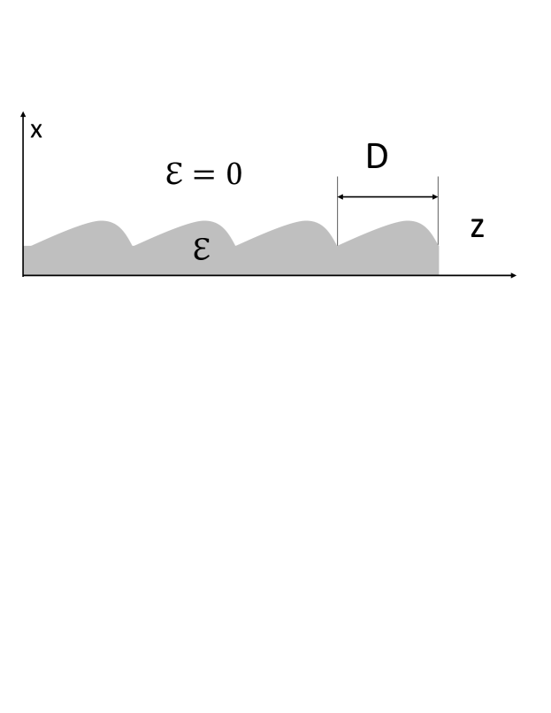
Figure 15: Grating geometry and notation.

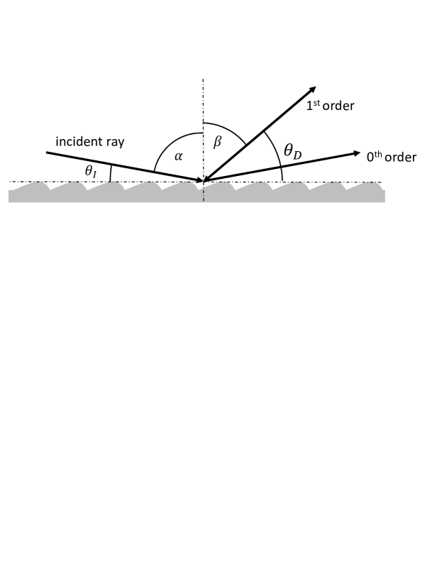
Figure 16: Scattering geometry for a diffraction grating.

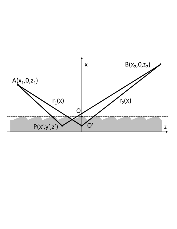
Figure 17: Schematic diagram of diffraction from a plane grating. The gray area represents the grating volume. A point source is located at A. Point P is an arbitrary point inside the grating volume. Grating can be divided into layers. Each layer is either homogeneous or modulated with refractive index that changes periodically as a function of $z$ at any given height $x$.

The derivation of the grating condition describing the geometry of light diffraction by gratings presented in textbooks usually relies on Huygens principle. At variance, our treatment of gratings theory is based on first principles, namely Maxwell equations, still retaining basic simplicity.

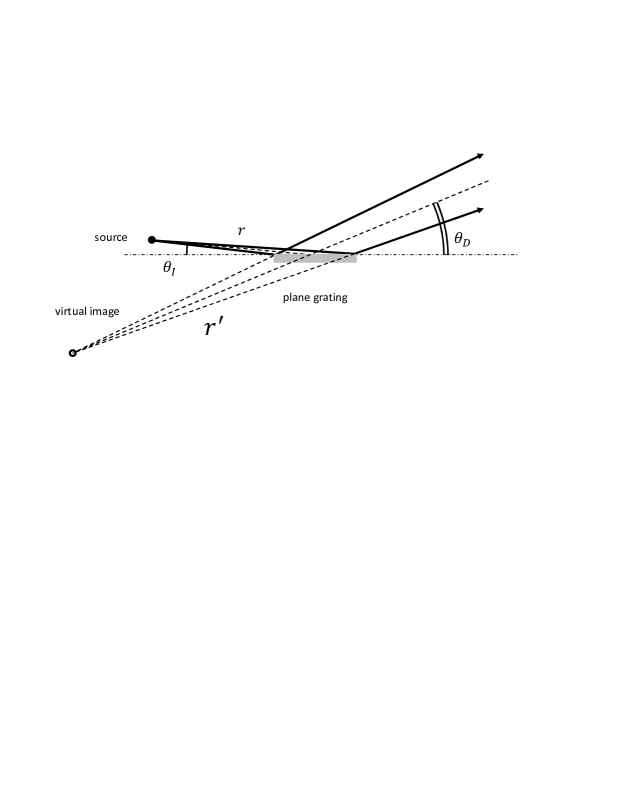
Figure 18: Plane grating in the case of a monochromatic point source. The virtual image of the real source is located at a distance $r^{\prime}=r\cdot\left(\sin(\theta_{D})/\sin(\theta_{I})\right)^{2}$ behind the grating.

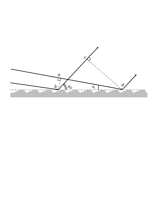
Figure 19: Geometry of the reflection. The properties of the grating are naturally described in terms of the asymmetry parameter $b=\sin(\theta_{D})/\sin(\theta_{I})$

Figure 20: Schematic diagram of a toroidal grating. A point source is located at A. Point P is an arbitrary point of the grating.

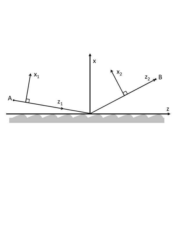
Figure 21: Coordinate notation. The coordinate systems $(x,y,z)$, $(x_{1},y_{1},z_{1})$ and $(x_{2},y_{2},z_{2})$ correspond to grating, incoming beam and diffracted beam; the axes $z$, $z_{1}$ and $z_{2}$ are along grating surface, incident and exit principal rays respectively.

Figure 22: Schematic diagram of a VLS grating element used in theoretical analysis. The VLS grating is represented by a contribution of a planar grating with fixed line spacing and a thin lens.

3.3.1 Plane grating

Ruled gratings are essentially two-dimensional structures. As such, their surface $S$ can be described by a function, e.g. $x=f(y,z)$, which expresses one of the three coordinates (in this case, $x$) as a function of the other two, Fig. 15. Let the beam be incident from vacuum ($x>0$) on the periodic cylindrical interface illustrated in Fig. 16. In this case, since S is cylindrical, $f$ can be considered as the only function of $z$ independently on the value of $y$, and one has that $x=f(z)$ is a periodic function of period $D$ (with spatial wave number $K=2\pi/D$). Susceptibility is a periodic function of $z$ and can be described by the Fourier series

$$\delta\epsilon=4\pi\chi=\sum_{m=-\infty}^{\infty}u_{m}(x)\exp[imKz]~{}.$$ (80)

We want to obtain a diffracted wave, which we express in its most general form as Eq. (64), from the knowledge of the field incident on the grating. Using the relation between $\vec{\bar{P}}$ and $\vec{\bar{E}}$, and the explicit expression for $G$ in Eq. (62) we can write the following integral equation for the electric field:

$$\vec{\bar{E}}_{d}(\vec{r})= k_{0}^{2}\int d\vec{r^{\prime}}\frac{\exp[ik_{0}|\vec{r}-\vec{r^{\prime}}|]}{|\vec{r}-\vec{r^{\prime}}|}\chi(x^{\prime},z^{\prime})$$ (82)

$$\times\left\{\left[\vec{\bar{E}}_{d}(\vec{r^{\prime}})+\vec{\bar{E}}_{i}(\vec{r^{\prime}})\right]-c^{2}\vec{n}\left[\vec{n}\cdot\left(\vec{\bar{E}}_{d}(\vec{r^{\prime}})+\vec{\bar{E}}_{i}(\vec{r^{\prime}})\right)\right]\right\}~{}.$$

It is customary to solve the scattering problem by a perturbation theory, assuming that at all points in the dielectric medium the diffracted field $\vec{E}_{d}$ is much smaller than the incident field $\vec{E}_{i}$. This allows one to neglect the diffracted electric field on the right hand side of Eq. (82) with the incident field $\vec{E}_{i}$, yielding

$$\vec{E}_{d}(\vec{r})=k_{0}^{2}\int d\vec{r^{\prime}}\frac{\exp[ik_{0}|\vec{r}-\vec{r^{\prime}}|]}{|\vec{r}-\vec{r^{\prime}}|}\chi(x^{\prime},z^{\prime})[\vec{E}_{i}(\vec{r^{\prime}})-c^{2}\vec{n}(\vec{n}\cdot\vec{E}_{i}(\vec{r^{\prime}}))]~{},$$ (83)

where for simplicity we neglected the bar in the notation for the field in the space-frequency domain.

In order to compute $\vec{E}_{d}$ in Eq. (83) we need to specify the incident field distribution $\vec{E}_{i}(\vec{r^{\prime}})$ within the dielectric medium. In fact, according to Eq. (83) the integration ranges over all coordinates $d\vec{r^{\prime}}$, but $\chi$ is different from zero inside the dielectric. Consider Fig. 17, where we sketch the geometry for our problem. Monochromatic light from a point source $A(x_{1},y_{1},z_{1})$ is incident on a point $P(x^{\prime},y^{\prime},z^{\prime})$ located into the grating, i.e. into our dielectric medium. Point $A$ is assumed, for simplicity, to lie in the $xz$ plane, i.e. $A=A(x_{1},0,z_{1})$. The plane $xz$ is called the tangential plane (or the principal plane, or the dispersive plane). The plane $yz$ is called the sagittal plane. As a first step we need to express the incident field $\vec{E}_{i}$, appearing in Eq. (83), at the generic point $P$ inside the dielectric. In order to do so, since we deal with a point source, we can take advantage of the spatial impulse response of free-space. As we have seen, this is nothing but the expression for a spherical wave originating from $A$

$$\vec{E}_{i}(x^{\prime},y^{\prime},z^{\prime})=E_{0}\frac{\exp[ik_{0}|\vec{r^{\prime}}-\vec{r}_{1}|]}{|\vec{r^{\prime}}-\vec{r}_{1}|}~{}.$$ (84)

After this, we consider that the beam is diffracted to the point $B=B(x_{2},0,z_{2})$. Mathematically, diffraction is taken care of by the Green’s function in Eq. (83), which represents a secondary source from point $P$. Finally, an explicit expression for $\chi$ is given in Eq. (80).

Even without explicit calculation of the integral in Eq. (83), a lot can be said analyzing the phase in the integrand. In fact, since integration in Eq. (83) involves an oscillatory integrand, the integrand does not contribute appreciably unless the arguments in the exponential functions vanishes. We therefore calculate the total phase in the integrand of Eq. (83), and analyze it.

Calculations can be simplified by applying the paraxial approximation. In fact, one can rely on it for writing expansions for $\overline{AP}=|\vec{r^{\prime}}-\vec{r}_{1}|$ and $\overline{PB}=|\vec{r}_{2}-\vec{r^{\prime}}|$ entering into the expression for the phase. This can be done in terms of the distances $r_{1}(x)=\overline{AO^{\prime}}$ and $r_{2}(x)=\overline{O^{\prime}B}$, where $O^{\prime}=(x^{\prime},0,0)$, $x^{\prime}$ being the x-coordinate of point $P$. However, further simplifications apply by noting that, in paraxial approximation, light actually traverses a very small portion of material with susceptibility $\chi$. The range of coordinates $x^{\prime}$, $y^{\prime}$, $z^{\prime}$ inside the grating is much smaller than the distances $r_{1}$ and $r_{2}$. In other words, the grating size and its thickness are much smaller than $r_{1}$ and $r_{2}$. Additionally, we assume that the grating thickness is much smaller than the relevant transverse size. Thus, we can neglect the dependence of distances $r_{1}$ and $r_{2}$ on $x^{\prime}$ in the expansion for the incident wave and in the Green function exponent, and use the approximations $r_{1}\simeq\overline{AO}$ and $r_{2}\simeq\overline{OB}$, where $O=(0,0,0)$ is a pole on the surface of grating, Fig. 17. Thus, the path $AOB$ defines the optical axis of the beam, and the angle of incidence and of diffraction, $\alpha$ and $\beta$ in Fig. 16, are simply following that optical axis. If points $A$ and $B$ lie on different sides of the $xz$ plane, angles $\alpha$ and $\beta$ have opposite sign.

Starting from the expressions

$$\overline{AP}^{2}=[r_{1}\sin\alpha+z^{\prime}]^{2}+y^{\prime 2}+[r_{1}\cos\alpha]^{2}~{},$$ (85)

$$\overline{PB}^{2}=[r_{2}\sin\beta+z^{\prime}]^{2}+y^{\prime 2}+[r_{2}\cos\beta]^{2}~{}.$$ (86)

and using a binominal expansion we can write the incident wave as

$$\vec{E}_{i}(x^{\prime},y^{\prime},z^{\prime})=$$ (87)

$$E_{0}\exp\left[ik_{0}\left(r_{1}+z^{\prime}\sin\alpha+\frac{z^{\prime 2}\cos^{2}\alpha}{2(r_{1}+z^{\prime}\sin\alpha)}+\frac{y^{\prime 2}}{2(r_{1}+z^{\prime}\sin\alpha)}\right)\right]=$$ (88)

$$E_{0}\exp\left[ik_{0}\left(r_{1}+z^{\prime}\sin\alpha+\frac{z^{\prime 2}\cos^{2}\alpha}{2r_{1}}+\frac{y^{\prime 2}}{2r_{1}}-\frac{z^{\prime 3}\sin\alpha\cos^{2}\alpha}{2r_{1}^{2}}-\frac{z^{\prime}y^{\prime 2}\sin\alpha}{2r_{1}^{2}}\right)\right],$$ (89)

(90)

The exponent of the Green function under the integral Eq. (83) as a function of the coordinates $x^{\prime}$, $y^{\prime}$ and $z^{\prime}$ of the point $P$ on the grating. From Fig. 17, one obtains

$$\exp[ik_{0}|\vec{r}-\vec{r^{\prime}}|]=$$ (91)

$$\exp\left[ik_{0}\left(r_{2}+z^{\prime}\sin\beta+\frac{z^{\prime 2}\cos^{2}\beta}{2(r_{2}+z^{\prime}\sin\beta)}+\frac{y^{\prime 2}}{2(r_{2}+z^{\prime}\sin\beta)}\right)\right]=$$ (92)

$$\exp\left[ik_{0}\left(r_{2}+z^{\prime}\sin\beta+\frac{z^{\prime 2}\cos^{2}\beta}{2r_{2}}+\frac{y^{\prime 2}}{2r_{2}}-\frac{z^{\prime 3}\sin\beta\cos^{2}\beta}{2r_{2}^{2}}-\frac{z^{\prime}y^{\prime 2}\sin\beta}{2r_{2}^{2}}\right)\right]~{},$$ (93)

(94)

We will now show that the periodic structure of the gratings restricts the continuous angular distribution of the diffracted waves to a discrete set of waves only, which satisfy the well-known grating condition. In order to do so, we insert Eq. (80), Eq. (90), and Eq. (94) into Eq. (83). As noticed above, the integrand does not contribute appreciably unless the arguments in the exponential functions vanishes. From Eq. (80), Eq. (90), and Eq. (94) it follows that the total phase in Eq. (83) can be expressed as a power series

$$\phi=k_{0}[r_{1}+r_{2}+C_{10}z^{\prime}+C_{20}z^{\prime 2}+C_{02}y^{\prime 2}+C_{30}z^{\prime 3}+C_{12}z^{\prime}y^{\prime 2}+...]~{}.$$ (95)

Typically, third order aberration theory is applied to the analysis of grating monochromators. In that case, the power series needs to include third order terms. The explicit expressions for the coefficients $C_{ij}$ are

$$C_{10}=\frac{nK}{k_{0}}+\sin\alpha+\sin\beta~{},$$ (96)

$$C_{20}=\frac{1}{2}\left[\frac{1}{r_{1}}\cos^{2}\alpha+\frac{1}{r_{2}}\cos^{2}\beta\right]~{},$$ (97)

$$C_{02}=\frac{1}{2}\left[\frac{1}{r_{1}}+\frac{1}{r_{2}}\right]~{},$$ (98)

$$C_{30}=-\frac{1}{2r_{1}^{2}}\sin\alpha\cos^{2}\alpha-\frac{1}{2r_{2}^{2}}\sin\beta\cos^{2}\beta~{},$$ (99)

$$C_{12}=-\frac{1}{2r_{1}^{2}}\sin\alpha-\frac{1}{2r_{2}^{2}}\sin\beta~{}.$$ (100)

$C_{20}$ and $C_{02}$ are the coefficients describing defocusing. $C_{30}$ describes the coma, and $C_{12}$ the astigmatic coma aberration. In practice, the most important ones are defocusing and coma. Ideal optics would require the phase $\phi$ to be independent of $z$.

Note that the presence of the term $nK/k_{0}$ in the $C_{10}$ coefficient directly follows from the insertion of Eq. (80) into Eq. (83). As said above, it is the periodic structure of the gratings which restricts the continuous angular distribution of the diffracted waves to a discrete set of waves. In order to find the direction of incident and diffracted beam, we impose the condition $C_{10}=0$, yielding:

$$nK+k_{0}(\sin\alpha+\sin\beta)=0~{}.$$ (101)

Eq. (101) is also valid for a plane mirror, if the grating period is taken equal to infinity. This fact can be seen inspecting Eq. (101), which yields $\alpha=-\beta$ for $D\longrightarrow\infty$, which is nothing but the law of mirror reflection.

Eq. (101) is known as the grating condition. This condition shows how the direction of incident and diffracted wave are related. Both signs of the diffraction order $n$ appearing into the equation are allowed. Assuming for simplicity diffraction into first order, i.e. $n=+1$, one has

$$\lambda=D(\cos\theta_{i}-\cos\theta_{d})~{},$$ (102)

where $\theta_{i}$ and $\theta_{d}$ are the angles between the grating surface and, respectively, the incident and the diffracted directions. By differentiating this equation in the case of a monochromatic beam one obtains

$$b=\frac{d\theta_{d}}{d\theta_{i}}=\frac{\sin\theta_{i}}{\sin\theta_{d}}$$ (103)

Note that $b=W_{i}/W_{d}$ is the ratio between the width of the incident and of the diffracted beam. Fig. 19 shows the geometry of this transformation. As has been pointed out elsewhere this is just the consequence of Liouville’s theorem.

The effect of the plane grating on the monochromatic beam is twofold: first, the source size is scaled by the asymmetry factor $b$ defined in Eq. (103) and, second, the distance between grating and virtual source behind the grating is scaled by the square of the asymmetry factor $b$, Fig. 18. In order to illustrate this fact, we consider a 1D Gaussian beam with an initially plane wavefront, described by the field amplitude (along a given polarization component) $\psi(x,0)=\ exp[-x^{2}/w_{0}^{2}]$. Assuming that the plane grating is positioned at $z$, the spatial spectrum of the Gaussian beam immediately in front of the grating, i.e. after propagation in free-space by a distance $z$ from the waist point, is given by

$$\psi(k_{x},z)=\sqrt{\pi}w_{0}\exp[ik_{0}z]\exp\left[-\frac{k_{x}^{2}w_{0}^{2}}{4}\right]\exp\left[-\frac{ik_{x}^{2}z}{2k_{0}}\right]~{}.$$ (104)

However, according to Eq. ((103)), the transformation of the angular spectrum performed by grating can be described with the help of $k^{\prime}_{x}=bk_{x}$, so that immediately after grating one obtains

$$\psi(k_{x},z)=\sqrt{\pi}w_{0}\exp[ik_{0}z]\exp\left[-\frac{k_{x}^{{}^{\prime}2}w_{0}^{2}}{4b^{2}}\right]\exp\left[-\frac{ik_{x}^{{}^{\prime}2}z}{2k_{0}b^{2}}\right]~{}.$$ (105)

We can interpret Eq. (105) in the following way: the Gaussian beam diffracted by the grating is characterized by a new virtual beam waist $w^{\prime}_{0}=w_{0}/b$ and by a new virtual propagation distance $z^{\prime}=z/b^{2}$. Introducing the dimensionless distance through the relation $z/L_{R}$, where $L_{R}$ is called the Rayleigh length, we can conclude that this dimensionless distance is invariant under the transformation induced by the plane grating.

The treatment of the diffraction grating given above yielded most of the important results needed for further analysis. In particular, it allowed us to derive the grating condition and it also allowed us to study the theory of grating aberrations. Our theoretical approach reaches into the foundation of electrodynamics, as is based on the use of Maxwell equations. Note that the treatment considered so far was carried out under the assumption of the validity of the first order perturbation theory, i.e. we assumed that for all the points in the dielectric medium, the diffracted field is negligible with respect to the incident field. The properties of the field actually exploited amount to the fact that in the $yz$ plane, the diffracted field has the same phase as the incident field plus an extra-phase contribution $nKz^{\prime}$. If we go up to second and higher orders in the perturbation theory we can see that this property remains valid, and results derived above still hold independently of the application of a perturbation theory. Note that inside the grating the beam is attenuated with a characteristic length that is much shorter compared to the range of the grating surface coordinates, and can always be neglected in the phase expansion. We can immediately extend the range of validity of our analysis to arbitrary values of the dielectric constant. The general proofs of the grating condition and of the results of the theory of grating aberration are derived from first principles as follows STRO .

First let us note that two-dimensional problems are essentially scalar in nature, and can be expressed in terms of only one single independent electromagnetic field variable, either $E_{y}$ or $H_{y}$. Here we will working considering the TE polarization, i.e. we will be focusing on $E_{y}$. The action of the grating on the electromagnetic field can be modeled, mathematically, as an operator $\mathcal{G}$ that transforms an incident field into a diffracted field, i.e. $E_{d}(z,y)=\mathcal{G}[E_{i}(z,y)]$. Since the grating is periodic and extends to infinity, the action of the operator $\mathcal{G}$ is invariant under translation by a grating period: $E_{d}(z+D,y)=\mathcal{G}[E_{i}(z+D,y)]$. Since the incoming beam is incident at an angle $\theta_{i}$, this translation adds an extra path distance $D\cos\theta_{i}$ to the incident wave $E_{i}$, for a phase change

$$E_{i}(z+D,y)=\exp(ik_{0}D\cos\theta_{i})E_{i}(z,y)~{}.$$ (106)

Also, since the set of Maxwell partial differential equations is linear, any solution multiplied by a constant is still a solution and one obtains

$$\mathcal{G}[E_{i}(z+D,y)]=\mathcal{G}[\exp(i\delta\phi)E_{i}(z,y)]=\exp(i\delta\phi)E_{i}(z,y)~{},$$ (107)

where $\delta\phi=k_{0}D\cos\theta_{i}$. Now, since

$$\mathcal{G}[E_{i}(z+D,y)]=E_{d}(z+D,y)$$ (108)

we must have

$$\exp(i\delta\phi)E_{d}(z,y)=E_{d}(z+D,y)~{}.$$ (109)

In other words, the diffracted field is a pseudo-periodic function. Now, since the product $E_{d}\exp[-ik_{0}z\cos\theta_{i}]$ is a periodic function, it can be represented as a Fourier series expansion on the grating period $D$, and we can write the diffracted field as

$$E_{d}(z,y)=\sum_{m=-\infty}^{+\infty}E_{m}(y)\exp[imKz+ik_{0}z\cos\theta_{i}]~{}.$$ (110)

This result is fully general, and all that is required to prove it is that the grating is periodic. Eq. (110) is sufficient for describing the geometry of the beam diffraction by the grating. We can use Eq. (110) to derive once more the grating condition.

In order to illustrate this fact, we see that the phase of the integrand in the integral Eq. (82) consists of three terms: the first term is the phase in the Green function, the second is the phase in Eq. (80), and the third is the phase in $\vec{E}_{d}$. The first and the second terms are known, and have already been analyzed. Eq. (110) shows the structure of the phase for $\vec{E}_{d}$ in the case for a plane wave impinging on the grating with incident angle $\theta_{i}$. In principle, the incident field $\vec{E}_{i}$ comes from a point source located in $A$, and consists of a diverging spherical wave. Such spherical wave can always been decomposed in plane waves and, due to the validity of the paraxial approximation, only those plane wave components with angle near to $\theta_{i}$ should be considered. Therefore, neglecting small corrections in $\Delta\theta_{i}$, one can take the phase in Eq. (110) as a good approximation for the phase of the diffracted field. Then, considering the expansion in Eq. (94) to the first order in $z^{\prime}$ one obtains, without using a perturbative approach, that the term in $z^{\prime}$ in the integrand in Eq. (82) is given by $(m+n)K+k_{0}(\cos\theta_{i}-\cos\theta_{d})$. Imposing that this term be zero, and remembering that $\alpha=\pi/2-\theta_{i}$, one gets back Eq. (101).

This result, albeit very general, still says nothing about the grating efficiency. We still do not know anything about the amplitudes of the diffracted waves. In order to determine these coefficients we need to model the grooves of the grating. At this point, we need to apply classical numerical integration techniques PETI , BOOT .

3.3.2 VLS plane grating

A diffractive plane grating can focus a diffracted beam when the groove spacing properly varies with the groove position; such a grating is called a variable-line-spacing (VLS) grating. A VLS plane grating can be incorporated into the monochromator to act as both dispersive and spectrally focusing component. The working principle of such kind of grating can be understood by expressing the groove spacing $D(z)$ as a function of the coordinate $z$ along the perpendicular to the grooves. So it can be expanded as a polynomial series:

$$D(z)=D_{0}+D_{1}z+D_{2}z^{2}+...~{},$$ (111)

where the term $D_{0}$ is the spacing at the pole of the grating (located, by definition, at $z=0$), while $D_{1}$ and $D_{2}$ are the parameters for the variation of the ruling with $z$. Now susceptibility is not a periodic function of $z$ anymore, and can be described by the Fourier integral:

$$\delta\epsilon=4\pi\chi=\int_{-\infty}^{\infty}B(K,x)\exp[iKz]dK~{}.$$ (112)

Let us assume, for simplicity, that the distance between grooves varies according to the linear law: $D(z)=D_{0}+D_{1}z$. Now we also assume that $D_{1}\ll 1$ and we apply the so-called adiabatic approximation imposing that the width of the peaks in the spectrum $B(K,x)$ is much narrower than the harmonic separation $K_{0}=2\pi/D_{0}$ between the peaks. In this case, Eq. (112) can be represented in the form

$$\delta\epsilon=\sum_{-\infty}^{+\infty}B_{n}(x,z)\exp[inK_{0}z]~{},$$ (113)

where the complex amplitudes $B_{n}(x,z)$ are all slowly varying function of the $z$ coordinate on the scale of the period $D_{0}$. This means that the terms in sum over $n$ in Eq. (113) can be analyzed separately for each value of $n$. For the case of a linearly chirped grating considered here, the slowly varying amplitude of the $n$th harmonic is given by

$$B_{n}=A_{n}(x)\exp\left[i\frac{z^{2}}{2}\frac{dK}{dz}\right]~{},$$ (114)

where $dK/dz=2\pi d(1/D)/dz=-(2\pi/D_{0}^{2})D_{1}$ is the chirp parameter.

We now substitute Eq. (113) into Eq.(83) and, as before, we express the phase in the integrand as a power series. Only the $C_{20}$ term differs, with respect to the expression in Eq. (100). In fact, for a linearly chirped grating we obtain ITOU

$$C_{20}=-\frac{\lambda}{2D_{0}^{2}}D_{1}+\frac{1}{2r_{1}}\cos^{2}\alpha+\frac{1}{2r_{2}}\cos^{2}\beta~{}.$$ (115)

The condition $C_{20}=0$ has to be verified in order to guarantee imaging in the tangential plane.

Here we used Maxwell equations for studying the imaging properties of VLS grating. However, certain aspects of this theory can be derived in a simple way using ray optics. For convenient use in the following discussions, it is necessary to make clear the reference coordinate systems and rays describing the optical system. Fig. 21 shows the VLS plane grating optical system with an object point $A$. The coordinate systems $(x,y,z)$ , $(x_{1},y_{1},z_{1})$ and $(x_{2},y_{2},z_{2})$ correspond, respectively, to the grating, to the incident beam, and to the diffracted beam; the axes $z$, $z_{1}$ and $z_{2}$ are along the grating surface, the incident and the exit principal rays, respectively. As shown in Fig. 16, the input beam is incident on grating at angle $\theta_{i}$. The diffracted angle $\theta_{d}$ is a function of the groove distances according to the grating equation

$$\lambda=D(\cos\theta_{i}-\cos\theta_{d})~{}.$$ (116)

By differentiating over $z$ for the case of a monochromatic beam we obtain

$$\frac{dD}{dz}(\cos\theta_{i}-\cos\theta_{d})=-\frac{d\theta_{d}}{dz}D\sin\theta_{d}~{},$$ (117)

yielding

$$[\lambda/D_{0}^{2}(\sin^{2}\theta_{d})]D_{1}=-\frac{d\theta_{d}}{dx_{2}}~{},$$ (118)

where we used the relation $z\sin\theta_{d}=x_{2}$.

Let us now define a thin lens as a device that deflects every light beam incident parallel to the optical axis in such a way that it crosses the optical axis at a fixed distance $f$ after passing through the lens. In paraxial approximation, the thin lens equation assumes the familiar form $d\theta_{d}=-dx_{2}/f$ . The physical meaning of Eq. (118) is that the VLS plane grating can be represented by a combination of a planar grating with fixed line spacing and a lens after the grating, with a focal length $f$ equal to the focal length of the VLS grating

$$f=[\lambda D_{1}/D_{0}^{2}(\sin^{2}\theta_{d})]^{-1}~{},$$ (119)

as shown in Fig. 21. It may seem surprising that the focal length depends on $\theta_{d}$ only. However, it is reasonable to expect an influence of the assumption that the lens placed after the grating. One intuitively expects that full transfer matrix for the VLS grating should not depend on the choice of the lens position. It will be shown below that indeed, the transfer matrix satisfies this invariance.

An ABCD matrix is intended to represent any arbitrary paraxial element, or optical system located between an input plane and an output plane. In the present case, the optical element is the VLS plane grating with the input plane corresponding to the plane perpendicular to the incident beam and with the output plane the plane perpendicular to the diffracted beam. The most usual application for ray matrices is to forming the image of the object The most usual application for ray matrices is the determination of the image of the object located at the input plane. In this case, some important properties of optical system are obtained when any of the ABCD parameters vanish MORE .

The total optical system from the object plane (to which point A belongs) to the image plane (to which point B belongs), see Fig. 21, is represented by the matrix:

$$\left(\begin{array}[]{l}A_{\mathrm{tot}}~{}~{}~{}~{}B_{\mathrm{tot}}\\ C_{\mathrm{tot}}~{}~{}~{}~{}D_{\mathrm{tot}}\end{array}\right)=\left(\begin{array}[]{l}1~{}~{}~{}~{}r_{2}\\ 0~{}~{}~{}~{}1\end{array}\right)\left(\begin{array}[]{l}1~{}~{}~{}~{}~{}~{}~{}~{}~{}~{}~{}0\\ -1/f~{}~{}~{}~{}1\end{array}\right)\left(\begin{array}[]{l}b~{}~{}~{}~{}~{}~{}0\\ 0~{}~{}~{}~{}1/b\end{array}\right)\left(\begin{array}[]{l}1~{}~{}~{}~{}r_{1}\\ 0~{}~{}~{}~{}1\end{array}\right)~{},$$ (130)

where $b$ is the asymmetric parameter $\sin\theta_{i}/\sin\theta_{d}$, see SIEG . The explicit expression for the total matrix elements are

$$A_{\mathrm{tot}}=b-br_{2}/f~{},$$ (131)

$$B_{\mathrm{tot}}=br_{1}-br_{1}r_{2}/f+r_{2}/b~{},$$ (132)

$$C_{\mathrm{tot}}=-b/f~{},$$ (133)

$$D_{\mathrm{tot}}=-br_{1}/f+1/b~{}.$$ (134)

The condition $B_{\mathrm{tot}}$ = 0 has to be verified in order to guarantee imaging of the object at the output plane. In fact, when $B_{\mathrm{tot}}=0$, any point source at the input plane focuses at the corresponding point in the output plane, regardless of the input angle. Therefore, the output plane is the image plane. Dividing the equation $B_{\mathrm{tot}}=0$ by $r_{1}r_{2}$ on the left hand side we find the imaging equation APRI

$$\frac{b}{r_{1}}+\frac{1}{br_{2}}=\frac{D_{1}\lambda}{D_{0}^{2}\sin\theta_{i}\sin\theta_{d}}~{},$$ (135)

which is identical to the imaging condition $C_{20}=0$ which we derived above from first principles, because $\sin\theta_{i}=\cos\alpha$ and $\sin\theta_{d}=\cos\beta$. It thus follows that the ABCD matrix for the VLS plane grating in the tangential plane has the general form

$$\left(\begin{array}[]{l}A_{\mathrm{tot}}~{}~{}~{}~{}B_{\mathrm{tot}}\\ C_{\mathrm{tot}}~{}~{}~{}~{}D_{\mathrm{tot}}\end{array}\right)=\left(\begin{array}[]{l}A_{\mathrm{tot}}~{}~{}~{}~{}~{}~{}~{}~{}0\\ -1/f_{\mathrm{tot}}~{}~{}~{}~{}D_{\mathrm{tot}}\end{array}\right)$$ (140)

with the effective focal length given by APRI

$$\frac{1}{f_{\mathrm{tot}}}=\frac{\lambda D_{1}}{D_{0}^{2}\sin\theta_{i}\sin\theta_{d}}~{},$$ (141)

which is symmetric in $\theta_{i}$ and $\theta_{d}$ as it must be. The ABCD matrix elements can be used to characterize width and wavefront curvature of the Gaussian beam after its propagation through the VLS grating.

3.3.3 Toroidal grating

A logical extension of the plane VLS grating concept described above follows from the idea to rule the VLS grooves on a toroidal surface, producing a toroidal VLS grating THOM . Additional design parameters, namely tangential and sagittal radius, are then available to control imaging aberrations and to optimize the grating monochromator performance HABE . We consider a curved VLS grating and we assume that the surface of the grating is toroidal with tangential and sagittal radius of curvature $R$ and $\rho$ respectively, see Fig. 20. Let us assume that the distance between the grooves varies according to quadratic law:

$$D(z)=D_{0}+D_{1}z+D_{2}z^{2}~{}.$$ (142)

As before, the susceptibility is not a periodic function with respect to $z$, and in adiabatic approximation can be represented in the form

$$\delta\epsilon=\sum_{-\infty}^{+\infty}B_{n}(x,z)\exp[inK_{0}z]~{},$$ (143)

which is identical to Eq. (113), where complex amplitudes $B_{n}$ are slowly varying functions of the $z$ coordinate on the scale of the period $D_{0}$. In the case of quadratically chirped grating, the $n$th amplitude is given by

$$B_{n}=A_{n}(x)\exp[iK^{\prime}z^{2}/2+iK^{\prime\prime}z^{3}/6]~{},$$ (144)

where

$$K^{\prime}=2\pi(1/D)^{\prime}=-2\pi D_{1}/D_{0}^{2}=2\pi n_{1}~{},$$ (145)

$$K^{\prime\prime}=2\pi(1/D)^{\prime\prime}=-4\pi[D_{2}/D_{0}^{2}-D_{1}^{2}/D_{0}^{3}]=4\pi n_{2}~{},$$ (146)

are the linear and quadratic chirp parameters.

From the geometry (see Fig. 20), and similarly as done before we can write

$$\overline{AP}^{2}=[r_{1}\sin\alpha+z]^{2}+y^{2}+[r_{1}\cos\alpha-x]^{2}~{},$$ (147)

$$\overline{PB}^{2}=[r_{2}\sin\beta+z]^{2}+y^{2}+[r_{2}\cos\beta-x]^{2}~{},$$ (148)

where the coordinate $x$ on the toroidal surface is related to $z$ and $y$ by the equation of the torus

$$x=R-R\left[1-\frac{z^{2}+y^{2}}{R^{2}}+2\frac{\rho}{R}\left(\frac{\rho}{R}-1\right)\left(1-\left(1-\frac{y^{2}}{\rho^{2}}\right)^{1/2}\right)\right]^{1/2}~{}.$$ (149)

The integrand in Eq. (83) is oscillatory, and does not contribute appreciably to the total integral unless the arguments of the exponential function vanishes. Using Eq. (83), Eq. (90) and Eq. (94), together with Eq. (143), Eq. (144), Eq. (148), and Eq. (149), it is then possible to expand the phase as a power series such as

$$\phi=k_{0}(r_{1}+r_{2}+C_{10}z+C_{20}z^{2}+C_{02}y^{2}+C_{30}z^{3}+C_{12}zy^{2}+...)~{}.$$ (150)

The explicit expressions for coefficients $C_{ij}$ are HARA

$$C_{10}=\frac{n\lambda}{D_{0}}+(\sin\alpha+\sin\beta)~{},$$ (151)

$$C_{20}=\frac{n\lambda n_{1}}{2}+\frac{1}{2}\left[\frac{\cos^{2}\alpha}{r_{1}}+\frac{\cos^{2}\beta}{r_{2}}-\frac{\cos\alpha}{R}-\frac{\cos\beta}{R}\right]~{},$$ (152)

$$C_{30}=\frac{n\lambda n_{2}}{3}-\frac{1}{2}\left[\left(\frac{\cos^{2}\alpha}{r_{1}}-\frac{\cos\alpha}{R}\right)\frac{\sin\alpha}{r_{1}}+\left(\frac{\cos^{2}\beta}{r_{2}}-\frac{\cos\beta}{R}\right)\frac{\sin\beta}{r_{2}}\right]~{},$$ (153)

$$C_{02}=\frac{1}{2}\left[\frac{1}{r_{1}}-\frac{\cos\alpha}{\rho}\right]+\frac{1}{2}\left[\frac{1}{r_{2}}-\frac{\cos\beta}{\rho}\right]~{},$$ (154)

$$C_{12}=-\frac{1}{2}\left[\left(\frac{1}{r_{1}}-\frac{\cos\alpha}{\rho}\right)\frac{\sin\alpha}{r_{1}}+\left(\frac{1}{r_{2}}-\frac{\cos\beta}{\rho}\right)\frac{\sin\beta}{r_{2}}\right]~{},$$ (155)

where the condition $C_{10}=0$ yields back the grating condition, $C_{20}=0$ yields the position of the tangential focus position, $C_{02}=0$ that of the sagittal focus, and the relation $C_{30}=0$ minimizes the coma aberration.

In section 4.3.4 we will demonstrate that toroidal grating aberrations can be modeled very straightforwardly using a geometrical approach. This derivation is very different from the analytical method used in literature. We heavily relied on geometrical considerations, and we hope that calculations performed in section 4.3.4 are sufficiently straightforward to give an intuitive understanding of Eq. (155).

4 Modeling of self-seeding setup with grating monochromator

4.1 Source properties

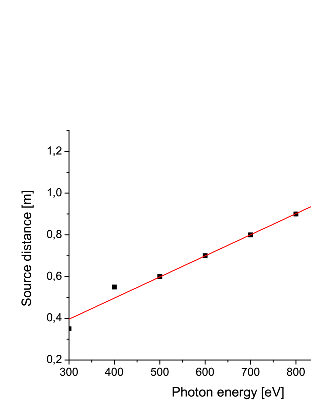
Figure 23: Distance of the source from the SASE undulator exit as a function of photon energy. Results are found by means of FEL simulations.

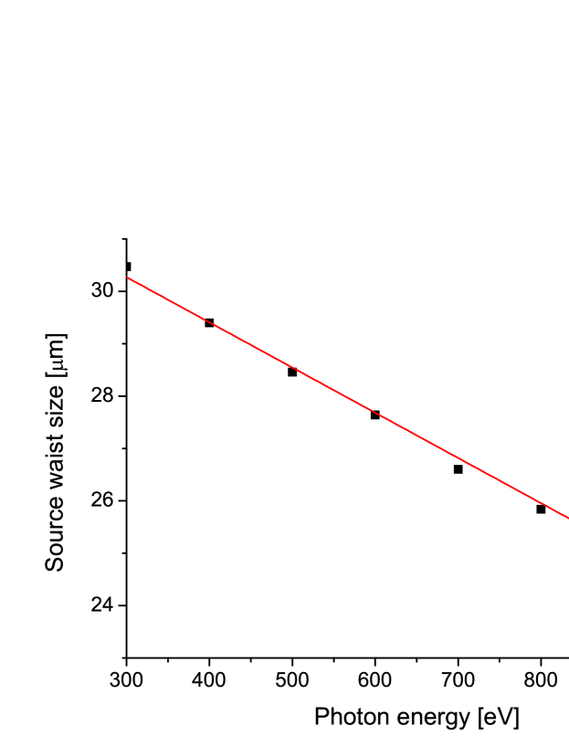
Figure 24: Size of the source waist as a function of the photon energy. Results found by means of FEL simulations.

In order to perform calculations of the grating beamline performance, one needs the effective source size and position through the operating photon energy range. The properties of the effective source are found from steady-state simulations with the help of the code Genesis 1.3 GENE . The simulations include electron beam parameters (emittance, energy spread, peak current) found by start-to-end simulations for the $0.1$ nC electron bunch mode of operation. Beam parameters for the steady-state simulations have to be chosen to match the parameters of the bunch slice with maximum peak current. The properties of the effective source can be found from the simulated field at the SASE undulator exit. This is accomplished by propagating the simulated field backwards from the undulator exit in order to find the position of the waist. The field must to be propagated in free-space. An in-house free-space wavefront propagation code was used to this purpose. The code is written in MATLAB and based on fast Fourier transform implementation of the Fourier optics method discussed in section 3.1. Fig. 23 shows the distance from the source to the SASE undulator exit as a function of the photon energy. It is seen that the source point moves upstream with increasing photon energy by as much as one meter. The Gaussian fit gives the source waist size $w_{0}$, as shown in Fig. 24.

4.2 Focusing at the second undulator entrance

Figure 25: Dependence of the input coupling factor A on the position of the Gaussian beam waist. Here $\hbar\omega=500$ eV.

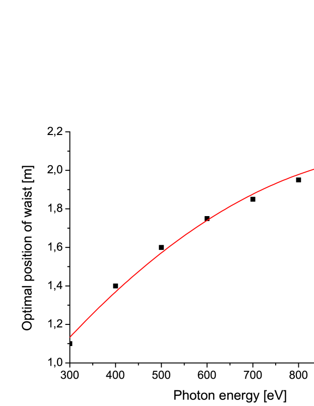
Figure 26: Optimal position of the Gaussian beam waist (characterized by plane wavefront) into the second undulator as a function of the photon energy. The waist size of the seed beam is equal to the source waist size in the first undulator. A usual figure of merit is the optimal position of the waist for the maximal input coupling factor. Results are obtained using wave optics and FEL simulations.

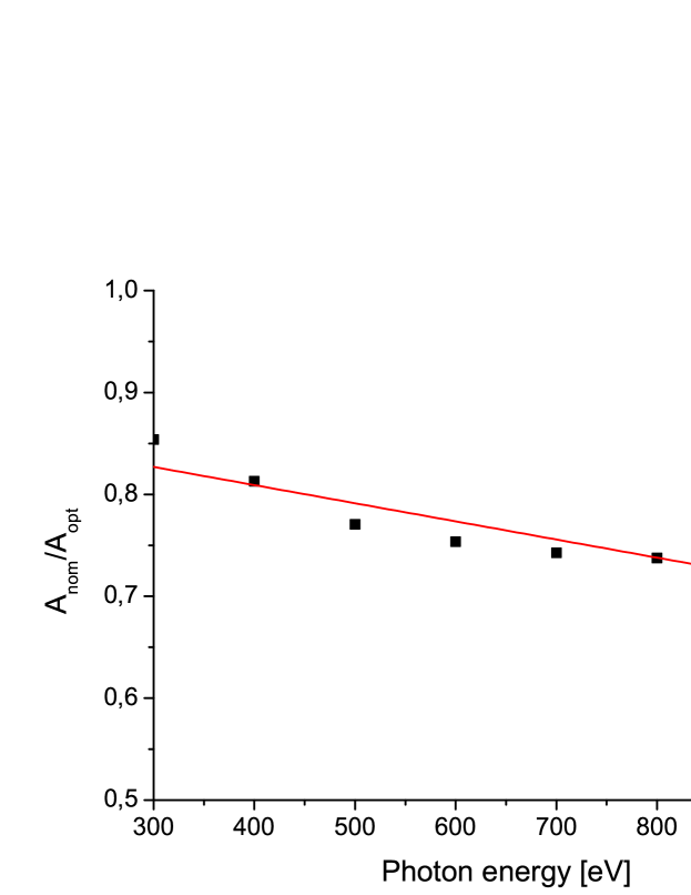
Figure 27: Ratio of input coupling factor for nominal and optimal seeding as a function of the photon energy.

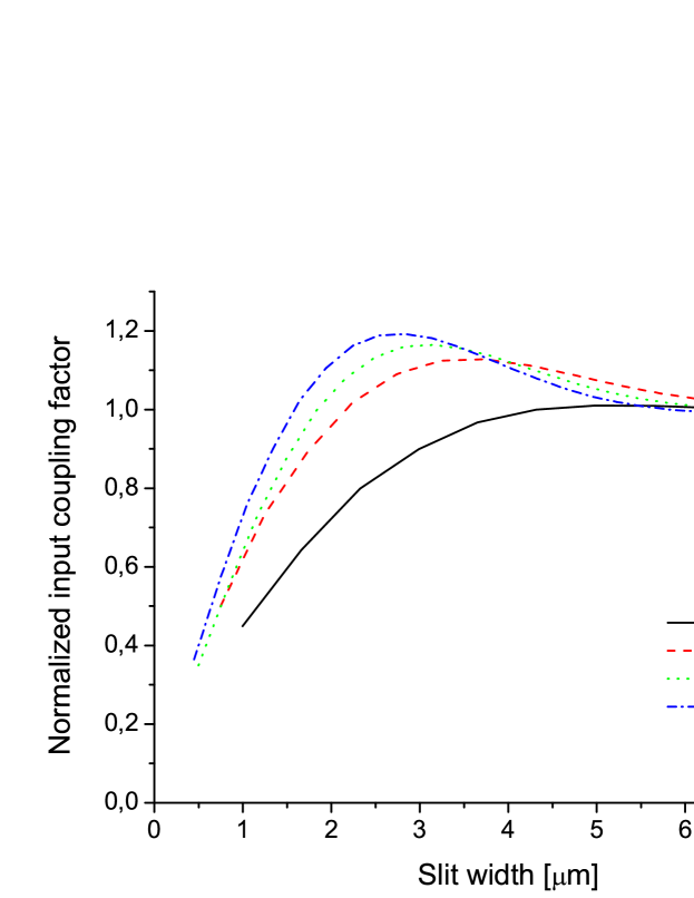
Figure 28: Transverse mismatch between monochromatic seed and electron beam as a function of exit slit width for different photon energies. A useful figure of merit measuring the mismatch is the input coupling factor normalized to the asymptotic case without exit slit. Results obtained using wave optics and FEL simulations.

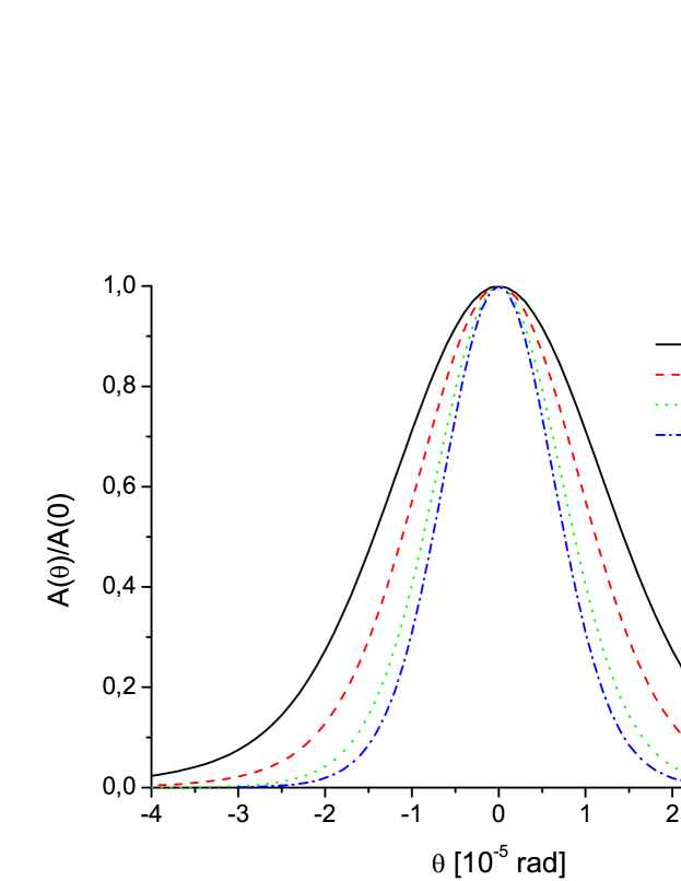
Figure 29: Results of FEL amplifier simulations showing the influence of the wavefront tilt in the seed beam. The normalized input coupling factor is plot as a function of the tilt angle for two photon energies.

Let us study the problem of optimal focusing of the seed radiation on the electron beam at the undulator entrance. We consider the case when the seed radiation has the form of a Gaussian beam, and when the FEL operates at exact resonance. The optimal focusing conditions can be found running steady-state simulations in Genesis 1.3 GENE .

The waist of the Gaussian beam is located at position $z_{0}$, where we have a plane phase front and a Gaussian distribution of amplitude. When the undulator is sufficiently long, the output power grows exponentially with undulator length, and the power gain, $G=W_{\mathrm{out}}/W_{\mathrm{seed}}$, can be written as

$$G=A\exp[z/L_{g}]~{},$$ (156)

where $z$ is the undulator length and $L_{g}$ is called the power gain length. In the linear regime the power gain does not depend on the input power $W_{\mathrm{seed}}$, so that the input coupling factor $A$ is a function of two parameters only: the coordinate of the waist location, $z_{0}$, and the waist size, $w_{0}$. There are always optimal values of Gaussian beam parameters, $w_{0}$ and $z_{0}$, when the input coupling factor $A$ achieves its maximum. In order to simplify the optimization problem, we will not study any change in $w_{0}$, but rather set it equal to the waist size of the effective source in the SASE undulator. Fig. 25 shows the dependence of the input coupling factor $A$ on the focus coordinate $z_{0}$ at the photon energy of $500$ eV. The optimal coordinate of the waist point is a function of the photon energy. The plot of this function is presented in Fig. 26. It is clearly seen that the optimal position of the waist located $1-2$ m inside the seeding undulator. The plots allow one to maximize the seeding efficiency at fixed power of the seed beam.

From the above analysis follows that that a one-to-one imaging of the radiation beam at the exit of the first undulator onto the entrance plane of the second undulator (which is obviously optimal in the case of negligible chicane influence) becomes non-optimal in the case of our interest. This is a consequence of the fact that the microbunching in the electron beam is washed out by the chicane and, therefore, at the entrance of the second undulator the seed radiation beam interacts with a ”fresh” electron beam. Numerical simulations show that the reduction factor for the one-to-one imaging case compared with the optimal case is about $30\%$.

The main efforts in developing our design for a self-seeding monochromator are focused on resolution and compactness. Therefore, there is somewhat a residual mismatching between seed and electron beam on the nominal mode of operation. From Fig. 27 one can see that seed beam on the nominal mode of operation is generated with a mismatching of only $10-20\%$ .

Wave optics, together with FEL simulations are naturally applicable also to the study the influence of finite slit size on the amplification process into the second undulator. In particular, we studied the influence of the exit slit size on the seeding efficiency. Such effect is shown in Fig. 7. One can see that decreasing the slit size drastically decreases the efficiency. The reason for this is a reduction of the seed power and the introduction of an additional mismatch between the seed beam and the electron beam. It is instructive to study these two effects separately. Fig. 28 shows the ratio of the input coupling factors for seeding with and without slit, as a function of the slit size. When the slit size is smaller than $2\mu$m, diffraction on the slit drastically decreases input coupling factor. On the other hand, for a slit size of about $2\mu$m, perturbation of the Gaussian beam shape leads to about $10-15\%$ increase in the input coupling factor.

In order to calculate the tolerance on the wavefront tilt of the seed beam, it is necessary to have knowledge of the angular acceptance of the FEL amplifier. Results of simulations performed with the code Genesis GENE are shown in Fig. 29. The minimum of the FWHM power amplification bandwidth ($0.2$ mrad) is achieved at the photon energy of $1$ keV.

4.3 Resolution

Figure 30: The number of illuminated grooves (number of grooves per waist of radiation beam illuminated) $N$ as a function of photon energy.

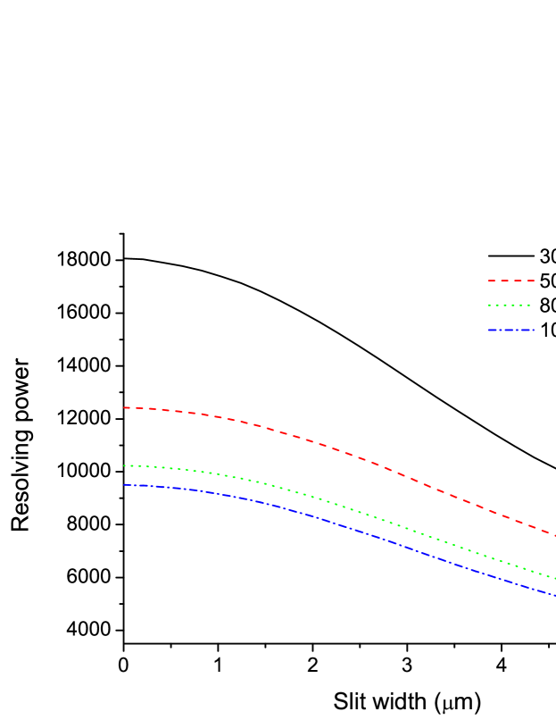
Figure 31: Resolving power of the grating monochromator as a function of the exit slit size for different photon energies.

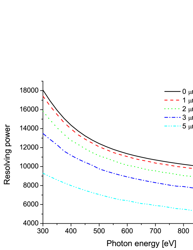
Figure 32: Resolving power of the grating monochromator as a function of the photon energy for different slit sizes.

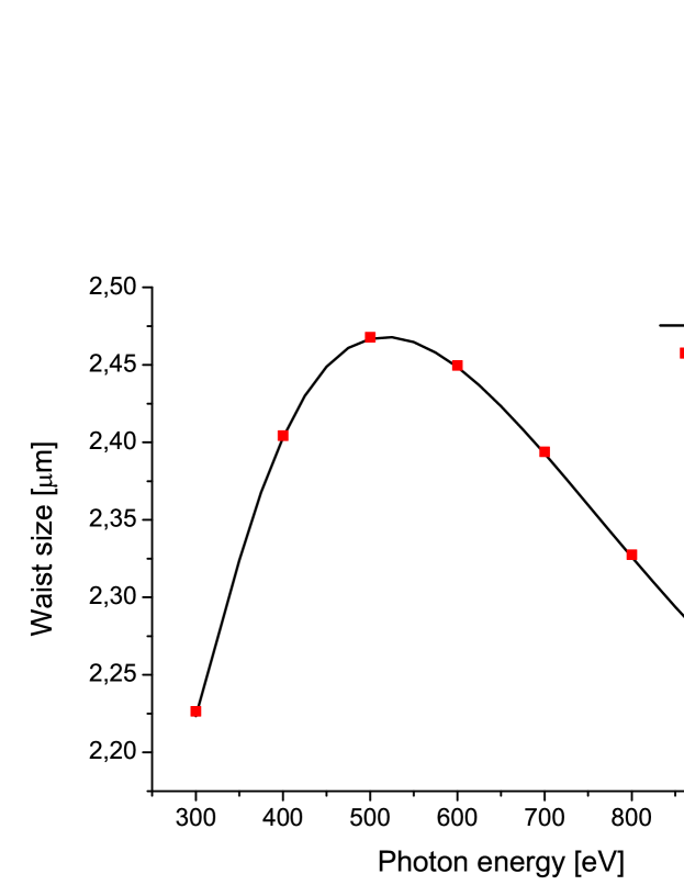
Figure 33: Image waist size on the exit-slit plane as a function of the photon energy. The curve are calculated with analytical formulas. Squares are the result of numerical calculations with the split-step beam propagation method.

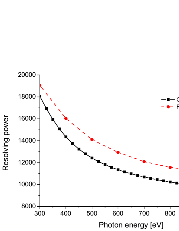
Figure 34: Maximal resolving power, i.e. resolving power at closed slits, as a function of photon energy. Results are obtained using wave optics calculations. Squares are calculated using coherent Gaussian beam, and circles are calculated using FEL beam.

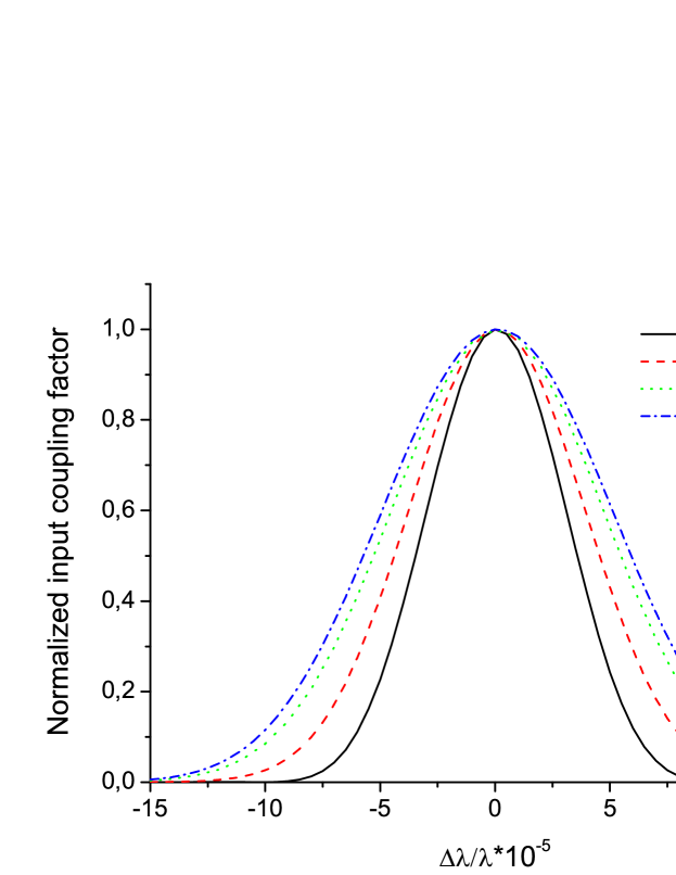
Figure 35: Profile of the output spectral line from the grating monochromator without exit slit at different photon energies. Results are obtained by wave optics and FEL simulations. The FWHM of the spectral line would indicates a resolving power of $7000$ in photon energy range $0.3$ keV - $1$ keV.

A preliminary resolution study was first performed using Gaussian optics calculations. Subsequently, in order to have a more realistic wave optics simulation, after using Gaussian beam treatment, the beam distribution was modeled using FEL simulations and accounting for third order optical aberrations.Optimized specifications have then been verified by ray-tracing simulations, accounting for all geometrical aberrations, as reported in the end of this section. The reason for first modeling the source as a Gaussian beam was to obtain a completely analytical, albeit approximated description of the self-seeding monochromator operation.

4.3.1 Analytical description

Let us first assume that the incident FEL beam is characterized by a Gaussian distribution. In this case, the ABCD matrix formalism is a powerful tool to describe the propagation of the beam through an arbitrary paraxial optical system. The optical system for the grating monochromator comprises grating, slit and mirrors spaced apart from each other. All these optical elements (grating, mirrors and free-space), with the exception of the slit, can be represented with the help of ABCD matrices, which can be used to characterize the width and the wavefront curvature of an optical Gaussian beam after its propagation through a grating monochromator without exit slit. Gaussian beam transformation due to mirrors, and translation in between mirrors can be tracked using the law for the transformation of $q$ in Eq. (38). It can be convenient to describe the diffraction of a Gaussian beam from a toroidal VLS grating using the ABCD matrix formalism too. The relevant geometry is shown in Fig. 20. The grating has a local groove spacing $D(z)=D_{0}+D_{1}z$ at a position z on the grating surface, a radius of curvature of the substrate $R$ in the tangential plane, and $\rho$ in the sagittal plane. In the tangential plane, a toroidal VLS grating can be represented by combination of a planar grating with fixed line spacing and lens after the grating, Fig. 22, with a focal length equal to the focal length of the toroidal VLS grating

$$f_{1}=\left[\frac{\lambda D_{1}}{D_{0}^{2}\sin^{2}\theta_{d}}+\frac{\sin\theta_{i}}{2R\sin^{2}\theta_{d}}+\frac{1}{2R\sin\theta_{d}}\right]^{-1}$$ (157)

In the sagittal plane the toroidal VLS grating can be represented by a single lens with a focal length

$$f_{2}=\left[\frac{\sin\theta_{i}}{2\rho}+\frac{\sin\theta_{d}}{2\rho}\right]^{-1}$$ (158)

In our analysis we calculate the propagation of the input signal to different planes of interest within the monochromator. We start by writing the input field in object plane, that is the source plane, as

$$\tilde{E}(x,y)=\exp\left[-\frac{x^{2}}{w_{0}^{2}}-\frac{y^{2}}{w_{0}^{2}}\right]~{}.$$ (159)

As shown in Fig. 16, the input beam is incident on the grating at the angle $\theta_{i}$. The diffracted beam emerges at an angle $\theta_{d}$, and is a function of the wavelength according to grating equation. Assuming diffraction into $n=+1$ order, one has

$$\lambda=D_{0}(\cos\theta_{i}-\cos\theta_{d})~{}.$$ (160)

By differentiating this equation one obtains

$$\frac{d\theta_{d}}{d\lambda}=\frac{1}{D_{0}\theta_{d}}~{},$$ (161)

where we assume grazing incidence geometry, $\theta_{i}\ll 1$ and $\theta_{d}\ll 1$. The physical meaning of this equation is that different spectral components of the outcoming beam travel in different directions. As said above, in the tangential plane the toroidal VLS grating is represented as combination of plane grating and convergent lens. We are interested in determining the intensity distribution in the image plane, i.e. at the slit position. The grating introduces angular dispersion, which the lens transforms into spatial dispersion in the slit plane. The spatial dispersion parameter, which describes the proportionality between spatial displacement and optical wavelength is given by

$$\eta=\lambda\frac{dx}{d\lambda}=\frac{d_{2}\lambda}{D_{0}\theta_{d}}~{},$$ (162)

where $d_{2}$ is the distance between grating and image plane. In our case study, the relative difference between focal length and image distance is about $1\%$. As a result one may approximately write $d_{2}=f_{1}$. The spectral resolution of the monochromator equipped with an exit slit depends on the spot size in the slit plane, is related with the individual wavelengths composing the beam, and with the rate of spatial dispersion with respect to the wavelength. For a Gaussian input beam, the intensity distribution in the waist plane, that is the slit plane, is given by $I=\exp(-2x^{2}/w_{s}^{2})$, where $w_{s}$ is the waist size on the slit. A properly defined merit function is indispensable for the design of a grating monochromator. A merit function based on the spread of the radiation spots is a suitable choice in our case of interest. Let us consider the limiting case of a slit with much narrower opening than the spot size of the beam for a fixed individual wavelength centered at $x=0$. In this case, the Gaussian instrumental function (i.e. the spectral line profile of the beam after monochromatization) is given by

$$I=\exp\left[-2\left(\frac{f_{1}\lambda}{w_{s}D_{0}\theta_{d}}\right)^{2}\left(\frac{\Delta\lambda}{\lambda}\right)^{2}\right]~{}.$$ (163)

The resolving power is often associated to the FWHM $\Delta\lambda$ of the instrumental function through the relation $R=\lambda/(\Delta\lambda)$. In our case of interest the resolving power is consequently given by

$$R=\frac{f_{1}\lambda}{1.18w_{s}D_{0}\theta_{d}}~{}.$$ (164)

The effect of a plane grating on the monochromatic beam is, as previously discussed, twofold: first, the source size is scaled by the asymmetry factor $b=\theta_{i}/\theta_{d}$ and, second, the distance between grating and virtual source before the grating is scaled by the square of the asymmetry factor. In our case, the waist of the virtual source $w^{\prime}_{0}$ and the distance $d^{\prime}_{1}$ are thus given by

$$w^{\prime}_{0}=w_{0}\theta_{d}/\theta_{i}~{},$$ (165)

$$d^{\prime}_{1}=d_{1}(\theta_{d}/\theta_{i})^{2}~{}.$$ (166)

After propagation through a distance $d_{2}$ behind the lens, the Gaussian beam is said to be focused at the point where it has a plane wavefront. Using Eq. (40), we obtain

$$w_{s}=\frac{w^{\prime}_{0}f_{1}}{[(d^{\prime}_{1}-f_{1})^{2}+z_{R}^{{}^{\prime}2}]^{1/2}}~{},$$ (167)

where $z^{\prime}_{R}=z_{R}(\theta_{d}/\theta_{i})^{2}$ is the Rayleigh range associated with the virtual source. In our case of interest, $f_{1}/d^{\prime}_{1}\sim 10^{-2}$, and the waist transforms as

$$w_{s}=w_{0}\frac{\theta_{i}}{\theta_{d}}\frac{f_{1}}{[d_{1}^{2}+z_{R}^{2}]^{1/2}}~{}.$$ (168)

Using this relation we can recast the expression for the resolving power in the form

$$R=\frac{\lambda z_{R}(1+d_{1}^{2}/z_{R}^{2})^{1/2}}{1.18w_{0}\theta_{i}D_{0}}=\frac{\pi w_{0}(1+d_{1}^{2}/z_{R}^{2})^{1/2}}{1.18\theta_{i}D_{0}}~{},$$ (169)

and with the help of Eq. (39), we finally obtain

$$R=\frac{\pi w_{g}}{1.18\theta_{i}D_{0}}~{},$$ (170)

where $w_{g}$ is the actual waist size of the Gaussian beam after propagation through a distance $d_{1}$, i.e in the plane immediately in front of the grating. In that plane beam has finite radius of curvature and its intensity is given by

$$I=I_{0}\exp\left[-2\frac{x^{2}}{w_{g}^{2}}\right].$$ (171)

We now introduce the new parameter $N=w_{g}/(D_{0}\theta_{i})$, which may be identified as the number of illuminated grooves within the projected beam-waist size $w_{g}/\theta_{i}$, and is related to the resolving power by

$$R=\frac{\pi N}{1.18}~{}.$$ (172)

The number of illuminated grooves is plotted against the photon energy in Fig. 30. Influencing factors include the variation of the source size, and the actual distance between source and grating.

We now turn to consider the case with an arbitrary slit width. Generally, the presence of the slit modifies the output spectrum, and the instrumental function is essentially a convolution of the diffraction-limited (Gaussian) instrumental function with the slit transmission function. As in the case for a diffraction-limited asymptotic, the resolving power is associated to the FWHM $\Delta\lambda$ of the instrumental function through the relation $R=\lambda/(\Delta\lambda)$. Fig. 31 and Fig. 32 illustrate the dependence of the resolving power on slit width and photon energy. Note that in our particular case study of self-seeding, the word ”resolving power” presented on Fig. 31 and Fig. 32 is to be understood in a narrow sense. Namely, as we will discuss below, the electron beam, which interacts with the seed beam into the second undulator, plays the role of the exit slit with some effective width, and this additional spectral filtering is always present. Here we are not to discuss about the overall modification of the output spectrum, but only about how the presence of the slit modifies the spectrum of the transmitted beam.

4.3.2 Simulations using beam propagation method

Above we analyzed the resolution of the grating monochromator using an analytical method. Here we show simulation results using the beam propagation method (BPM). We used a in-house developed MATLAB code that calculates the propagation of the monoenergetic beam through the monochromator. The accuracy of the beam propagation method could be tested with analytical results for the Gaussian beam approximation. We simulated the focusing of the Gaussian beam by a toroidal VLS grating on the exit slit. Fig. 33 shows the dependence of waist size as a function of photon energy. From Fig. 33 it can be seen that there is a good agreement between numerical and analytical results.

Most of the results presented in this article were obtained in the framework of a Gaussian beam model. This is a very fruitful approach, allowing one to study many features of the self-seeding monochromator by means of relatively simple tools. However, it is relevant to make some remarks on the applicability of the Gaussian beam model. In practical situations the FEL beam has no Gaussian distribution, and the question arises whether a Gaussian approximation yields a correct design for a self-seeding monochromator. We therefore performed the same analysis using BPM simulations. With the help of the plots presented in Fig. 34 one can give a quantitative answer to the question of the accuracy of the Gaussian beam model. Numerical simulations for the monochromator have been performed in the steady-state FEL beam approximation using geometry parameters (in particular, the position of the slit) obtained from the Gaussian beam approximation. One can see that the the characteristics of the monochromator designed using a Gaussian beam approach do not differ significantly from those based on a model exploiting steady-state FEL beam distribution.

4.3.3 Modeling the monochromator without slit

When describing the operation of the self-seeding setup, we always considered the exit slit as spectral filter. However, to some extent this is a simplification since in reality, for sufficiently large slit sizes, the filtering is automatically produced by the second FEL amplifier. In fact, the angular dispersion of the grating causes a separation of different optical frequencies at the entrance of the second undulator. The spectral resolution without slit depends on the radiation spot-size at the entrance of the second undulator related with individual frequencies, and on the rate of the spatial dispersion with respect to frequencies. The center frequency of the passband filter is determined by the transverse position of the electron beam. The resolving power is limited by the electron beam transverse size, and can be high in the whole photon energy range covered by the monochromator. This mode of operation has the an advantage. In fact, it is important to maximize the transmission through the monochromator in order to preserve both the beam power and the transverse beam shape. It can easily be demonstrated that such beam power loss and mismatching are minimized when the monochromator operates without a slit.

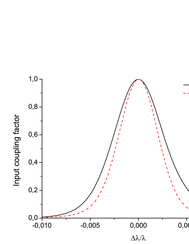
Figure 36: Input coupling factor as a function of wavelength detuning.

It is important to quantitatively analyze this filtering process. The influence of the spatial dispersion at the entrance of the second undulator on the operation of the self-seeding setup can be quantified by studying the input coupling factor between seed beam and FEL amplifier. In the linear regime, the input coupling factor $A$ can be found independently for each individual frequency, and allows for a convenient measure of the influence of the seed-beam displacement. In practice, it is sufficient to consider the limiting case of an instrumental function bandwidth ($\sim 0.02\%$) much narrower than the FEL amplification bandwidth ($\sim 0.5\%$). In this case the resolution is defined by the response of the FEL amplifier power on the seed displacement in the case of a monochromatic beam transmitted through the monochromator without slit. A spatial dispersion parameter, which describes the proportionality between spatial displacement and frequency at the entrance of the second undulator, can be found by monochromator simulations using our BPM code. The instrumental functions of the self-seeding setup without slit for different photon energies are presented in Fig. 35. In order to calculate the tolerance on the frequency detuning of the seed beam, it is necessary to have knowledge of the frequency response of the FEL amplifier. Results of simulations are shown in Fig. 36.

4.3.4 Method for computing third order aberrations for a toroidal grating

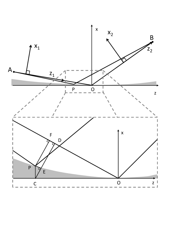
Figure 37: Optical scheme and coordinate systems for a toroidal grating system. The lower sketch is an enlarged fraction of the upper one.

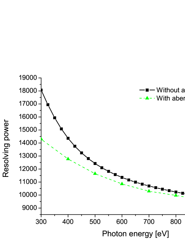
Figure 38: Resolving power of the grating monochromator at closed slit as a function of the photon energy. Results are obtained using wave optics calculations. Squares are calculated for an optical system without aberrations, and triangles are results for an aberrated optical system.

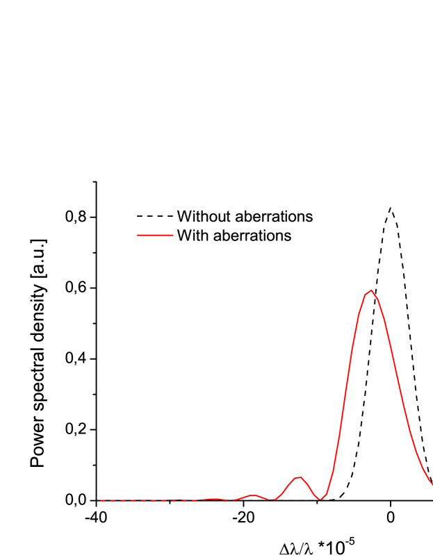
Figure 39: Effect of aberrations on the monochromator performance. Results are obtained using wave optics calculations. Simulations of the instrumental function at closed exit slit for aberrated and non-aberrated optical system are compared. Here $\hbar\omega=300$ eV.

In this paragraph we study the theory of third-order aberrations theory for a toroidal grating. It is first necessary to clearly define the reference coordinate systems used to describe the optical system. Fig. 37 shows the toroidal grating and the object point $A$. The three coordinate systems $(x,y,z)$, $(x_{1},y_{1},z_{1})$, and $(x_{2},y_{2},z_{2})$ are used to describe the position of the wave on the optical surface, the incoming wavefront and the diffracted wavefront, respectively. The ray AOB is referred to as the principal ray. In the following, the wavefront aberrations, the positions of the object and image plane are specified with respect to this ray. The wavefront aberration $W$ for a spherical wave passing through a point $P$ in the system is defined as the path difference between the principal and auxiliary ray: $W=\overline{APB}-\overline{AOB}$. Here we take advantage of the paraxial approximation obtained by ignoring all terms but the first quadratic terms in $x_{1}$ and $y_{1}$. Let us assume that point $A$ is in the tangential plane and $P(x_{1},0,z_{1})$ is any point on the grating surface satisfying the constraint $y_{1}=0$. The equation for the path $\overline{AP}$ is

$$\overline{AP}=z_{1}+\frac{x_{1}^{2}}{2z_{1}}=\overline{AF}+\frac{\overline{PF}^{2}}{2\overline{AF}}~{},$$ (173)

where $\overline{AF}=\overline{AO}-\overline{OD}-\overline{FD}$, $\overline{OD}=|z|\cos\alpha$, $\overline{FD}=x\cos\alpha$, $\overline{PF}=\overline{CD}-\overline{CE}=|z|\cos\alpha-x\sin\alpha$. Here $(x,y,z)$ are the coordinates of the point $P$ in the grating coordinate system and the coordinate system is chosen in such a way that $x>0$. Neglecting all terms of order higher than the second in $x$ and $y$, the form of a toroidal surface can be expressed by the equation

$$x=\frac{z^{2}}{2R}+\frac{y^{2}}{2\rho}~{},$$ (174)

where $R$ and $\rho$ are tangential and sagittal radius of curvature. Thus, the distance $PC$ is given by $x=z^{2}/(2R)$. Finally, we have

$$\overline{AP}-\overline{AO}=z\sin\alpha-\frac{z^{2}}{2R}\cos\alpha+\frac{\left[z\cos\alpha+z^{2}\sin\alpha/(2R)\right]^{2}}{2\left[r_{1}+z\sin\alpha-z^{2}\cos\alpha/(2R)\right]}~{},$$ (175)

where we used the notation $\overline{AO}=r_{1}$. Expanding this last difference as a power series in $z$ including the third order yields

$$\overline{AP}-r_{1}=$$ (176)

$$z\sin\alpha+\frac{z^{2}}{2r_{1}}\cos^{2}\alpha-\frac{z^{2}}{2R}\cos\alpha-\frac{z^{3}}{2r_{1}^{2}}\sin\alpha\cos^{2}\alpha+\frac{z^{3}}{2Rr_{1}}\cos\alpha\sin\alpha~{}.$$ (177)

(178)

Extension to the case of nonzero sagittal coordinate can be derived in the same way as above and results into an additional term $\Delta T$

$$\Delta T=\frac{y_{1}^{2}}{2z_{1}}=\frac{y^{2}}{2r_{1}}+\frac{y^{2}}{2\rho}\cos\alpha-\frac{y^{2}z}{2r_{1}^{2}}\sin\alpha~{}.$$ (179)

Note that the difference $\overline{BP}-\overline{BO}$ can be obtained following the same procedure described above, simply replacing the incidence angle $\alpha$ with the diffraction angle $\beta$. From Eq. (178), Eq. (179), Eq. (150), and Eq. (155) one obtains that the power series of $z$ and $y$ are identical.

In the previous sections, we studied the monochromator performance using a beam propagation method. We performed simulations in the framework of a simple model. Toroidal VLS grating was represented by a combination of a planar grating with a fixed line spacing and a lens after the grating. A BPM code was used to describe the propagation of a beam with an arbitrary initial field distribution through a paraxial system which was a combination of free-space, lens and plane grating with fixed line spacing. The problem to be solved now, is how to account for third order aberrations in the frame of the BPM code. In the case of a point source this problem has simple solution. Propagation from point source for a distance $r_{1}$ from the grating, reflection from the grating, and subsequent propagation to the image plane along a distance $r_{2}$ from the grating becomes similar to propagation through a plane grating with fixed line spacing, an ideal thin lens and an additional transparency at the lens position, which changes the phase of the reflected beam according to

$$\delta\phi=k_{0}C_{30}z^{3}+k_{0}C_{12}zy^{2}=k_{0}C_{30}\left(\frac{x_{2}}{\theta_{d}}\right)^{3}+k_{0}C_{12}\left(\frac{x_{2}}{\theta_{d}}\right)y_{2}^{2}~{},$$ (180)

where $x_{2}$ and $y_{2}$ are the coordinates of the wavefront immediately behind the grating. Generally, in order to obtain the output field distribution at a distance $z$ away from the input in the paraxial approximation, we need to convolve the input field distribution with the spatial impulse response

$$h(x-x^{\prime},y-y^{\prime},z)\sim\exp\left[-ik_{0}\frac{(x-x^{\prime})^{2}+(y-y^{\prime})^{2}}{2z}\right]~{},$$ (181)

and the above-described method to account for third order aberrations is not applicable. The case with finite source size is more complicated, and should be studied separately. However, in the far-zone approximation, which is our case of practical interest, the ratio between source size and beam size in the plane immediately in front of the grating is relatively small. Also, the image size is much smaller than the beam size in the plane immediately behind the grating. As a result, the algorithm described above is applicable. In this way, third order aberrations can be included into our study.

Fig. 38 shows a plot of the resolving power derived from BPM code accounting for aberrations. Clearly, the performance is limited by aberrations only at low photon energies close to $300$ eV. Fig. 39 illustrates the influence of aberrations on the lineshape at the photon energy of $300$ eV. The profile is highly asymmetric, owing to aberrations dominated by the primary coma.

4.4 Beamline efficiency

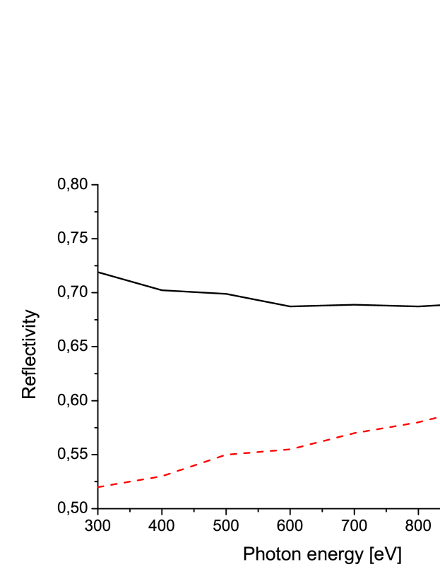
Figure 40: Reflectivity of the post-grating optical components of the beamline. The solid line shows the combined effect of the last two fixed-angle mirrors. The dashed line represents the reflectivity of the rotation mirror $M1$.

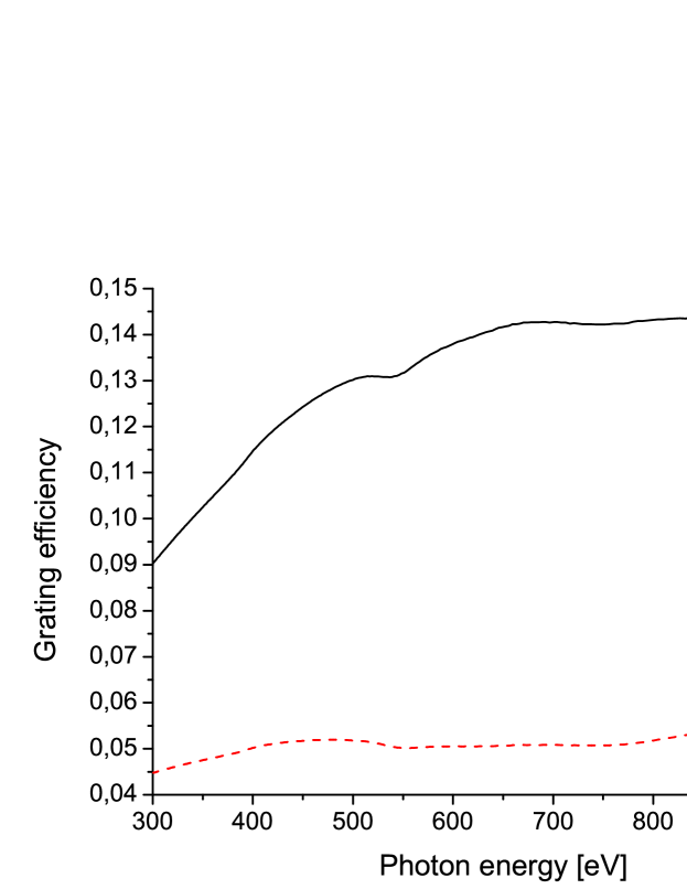
Figure 41: First order efficiency for two different groove profiles. In both cases, the groove density is $1100$ lines/mm, Pt coating is assumed. The incidence angle is $1^{\circ}$. Lamellar grating (rectangular): $11$ nm groove depth, 50% duty cycle. Blazed grating: $1,2^{\circ}$ blaze angle, $90^{\circ}$ anti-blaze angle.

Figure 42: Overall efficiency of the monochromator beamline without exit slit as a function of the photon energy. The grating and the three mirrors are platinum-coated.

It is important to calculate the expected total reflectivity of the monochromator beamline. The reflectivity of the mirrors was calculated using the code CXRO CXRO . Mirrors are assumed to be platinum-coated. The reflectivity of post grating optical components are shown in Fig. 40 as a function of the photon energy. The combining effect of two fixed angle mirrors cannot be neglected. In the soft X-ray range, platinum has reflectivity of about $92\%$ at $0.86$ degree grazing angle. The compound loss over two last reflections is thus appreciable. The most significant single factor in the post grating efficiency is, as expected, the low reflectivity of the rotating plane mirror $M1$. This is because the first post-grating mirror operates at a relatively large incident angle of about $2$ degrees. The grating efficiency was calculated using the code GSolver 5.2 GSOL . For comparison, Fig. 41 shows the first order efficiency for two typically-used grating profiles, blazed and laminar. Both gratings have a groove density of $1120$ lines/mm, are considered to operate at an incidence angle of $1^{\circ}$, and have had their geometry optimized for maximum efficiency in the first order. Gratings are also assumed to be platinum-coated. The blazed grating was optimized by adjusting the blaze angle and the laminar grating by adjusting the groove depth. A laminar profile is widely used due to its good suppression of the second and higher diffraction orders. A blazed profile is preferable from the point of view of absolute efficiency. Since the necessity of high seed power at the entrance of the second undulator and harmonic contributions are not an issue, the blazed profile has been chosen. The total reflectivity of the beamline with blazed grating is shown in Fig. 42. This reflectivity refers to the $\pi$-polarization component. The beamline reflectivity for the $\sigma$-polarization component is not significantly different.

4.5 Energy tuning and optical delay

Figure 43: Optical delay caused by the use of monochromator as a function of photon energy.

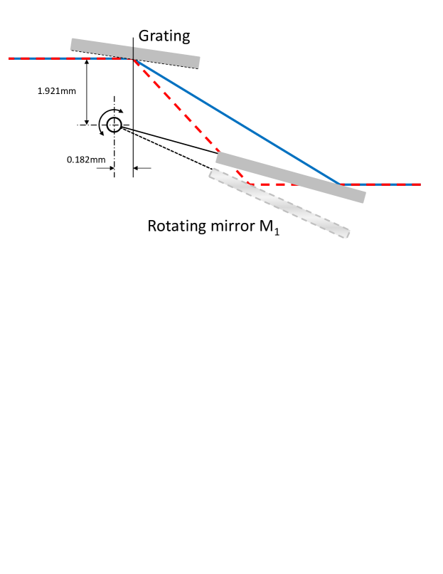
Figure 44: Principle of photon energy tuning. A plane scanning mirror, $M_{1}$, is rotated to maintain a fixed exit beam direction and focal spot at the exit slit. The mirror $M_{1}$ and grating are schematically shown for two photon energies: 1 keV (solid) and 0.5 keV (dashed line).

In order to maintain a constant direction of the exit beam, a scanning post grating mirror is placed in the diffracted beam, and rotated to direct the beam towards the exit slit. Thus, with a fixed grating and exit slit one can maintain a good focus over a wide photon energy range by simply translating and rotating a plane mirror to aim the diffracted light at the exit slit. Translating the mirror during rotation scanning can be achieved by pivoting the mirror at a point above the center of the mirror. During the energy tuning the beam walks along the surface of $M1$, as shown in Fig. 44. The optical delay caused by the use of the grating monochromator is about $0.7$ ps and its energy-dependence is shown in Fig. 43. The delay is not constant, but varies with the energy due to the fact that X-rays reflect off the post-grating mirror $M1$ at different points, and take different optical paths as the energy is tuned. The image on the slit plane is also found to vary by $1~{}\mu$m in the dispersion direction, amounting to a change of $1~{}\mu$rad in the angle of incidence, which is small compared to the divergence of the beam at the slit plane. As such, the impact of this effect on the monochromator performance is negligible.

4.6 Effects of mirror surface errors

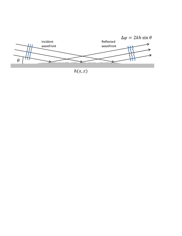
Figure 45: Thin-shifter-like behavior of surface roughness for small mean square of surface displacement, adapted from BART .

Figure 46: Distribution of residual height error and one-dimensional power spectral density (1D PSD) for the mirrors. The upper graph shows the height error profile for a $10$ cm-long plane mirror M1. The lower graph is the 1D PSD corresponding to the profile.

Figure 47: Effect of surface roughness on the monochromator performance. Simulations of the instrumental function at closed slit for different root-mean-square of surface displacements are shown in the figure. Here $\hbar\omega=1$ keV.

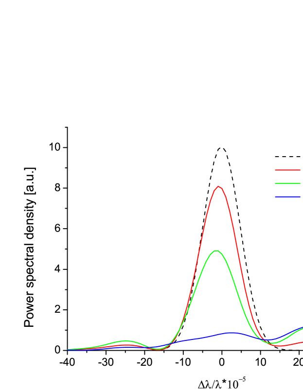
Figure 48: Effect of surface roughness on the monochromator performance. Simulations of the instrumental function without exit slit for different root-mean-square of surface displacements. Here $\hbar\omega=1$ keV.

A very important issue is the preservation of the radiation wavefront from the source to the entrance of the second undulator. Estimates of the requirements on the mirror for grating monochromators are usually based on ray-tracing codes for incoherent light sources. Since the XFEL beam will be almost transform-limited, one needs to perform simulations of the effect of the mirror imperfections by wavefront propagation codes. It is easy to demonstrate that an error $\delta h$ on the optical surface will perturb the wavefront of a phase $\phi$, according to

$$\phi=\frac{4\pi\delta h}{\lambda}\sin\theta_{i}~{},$$ (182)

where $\theta_{i}$ is the angle of incidence with respect to the surface. In the case of a grating, the phase shift can be expressed in terms of incidence and diffracted angles:

$$\phi=2\pi(\sin\theta_{i}+\sin\theta_{d})\frac{\delta h}{\lambda}~{}.$$ (183)

In practice, $\phi$ represents the deformation of the wavefront in the propagation direction divided by the wavelength.

A reflection from the mirror becomes similar to the propagation through a transparency at the mirror position, which just changes the phase of the reflected beam without changing its amplitude, BART (see Fig. 45). For the shifter model to be applicable, the phase change must be small, i.e. $|\phi|<<1$. Optical elements were modeled as a phase shifters, and the problem of simulating a monochromator was reduced to the proper description of the phase shifters and of the propagation of the wavefront in vacuum between the phase shifters. The main wavefront distortion at the slit position and at the entrance of the second undulator originates from the grating and the plane mirror $M1$. Applying the Marechal criterion, i.e. requiring a Strehl ratio larger than $0.8$, and treating the errors from the different optics independently, we obtain the following condition for the rms height error $h_{\mathrm{rms}}$ HEIM :

$$2h_{\mathrm{rms}}\theta_{i}\sqrt{N}<\lambda/14~{},$$ (184)

where $\theta_{i}$ is the grazing angle of incidence and $N$ is the number of optical elements. The most tight requirements corresponds to shortest wavelength. The grating operates at a fixed incidence angle $\theta_{i}=1$ degree, and at $1$ keV photon energy, the diffraction angle is about $3.2$ degrees. This corresponds to an incidence angle $(\theta_{i}+\theta_{d})/2=2.2$ degree for the mirror $M1$. From Marechal criterion we conclude that a height error $h_{\mathrm{rms}}=1$ nm should be sufficient for diffraction-limited monochromatization at the photon energy of $1$ keV. This is a very tight requirement. State-of-the art manufacturing achieves routinely rms values of $2$ nm for $10$ cm-long mirrors and one needs to perform detailed simulations of the surface error effect for understanding the requirements on the roughness.

The surface errors were generated from power spectral density (PSD) functions described in mirrors specifications. The part of the PSD, which makes the most significant contribution to the overall rms height error, is the low spatial-frequency part. An example of profile and PSD of mirror surface errors is shown in Fig. 46. Due to the very small incident angle, the beam footprint is much larger in the tangential direction than in the sagittal direction. The lowest spatial frequency that contributes is in order of $\theta_{i}/w\sim 1/$cm in the tangential direction. Here $w$ is the beam size at the optical element. It follows that the grating and the mirrors will disturb the wavefront mainly in the tangential direction. Simulations were performed using a BPM code. The surface figure can be directly mapped onto the optical field coordinate system using the geometrical transformation described above. Examples of the simulated focus at the exit slit for $1$ nm, $2$ nm and $4$ nm rms quality optics are presented in Fig. 47. Non Gaussian tails are seen on the sides of the instrumental function. The influence of surface errors on the resolution in the case when the slit is absent is shown in Fig. 48. An rms roughness of order of $2$ nm seems at present to be acceptable for the self-seeding setup.

4.7 Ray-tracing results

Figure 49: Results from ray tracing simulations at the plane of the exit slit for three photon energies $999.8$ eV, $1000.0$ eV and $1000.2$ eV, obtained from the ray-tracing program SHADOW. The histograms show the number of rays as a function of $x$ and $y$ coordinates. From the separation of the photon energies, a resolving power of $5000$ would be expected.

Figure 50: Results from ray tracing simulations at the plane of the exit slit for three photon energies $499.9$ eV, $500.0$ eV and $500.1$ eV, obtained from the ray-tracing program SHADOW. The histograms show the number of rays as a function of $x$ and $y$ coordinates. From the separation of the photon energies, a resolving power of $5000$ would be expected.

Figure 51: Results from ray tracing simulations at the entrance of the second undulator for three photon energies $999.8$ eV, $1000.0$ eV and $1000.2$ eV, obtained from the ray-tracing program SHADOW. The histograms show the number of rays as a function of $x$ and $y$ coordinates. From the separation of the photon energies, a resolving power of $5000$ would be expected.

Figure 52: Results from ray tracing simulations at the entrance of the second undulator for three photon energies $499.9$ eV, $500.0$ eV and $500.1$ eV obtained from the ray-tracing program SHADOW. The histograms show the number of rays as a function of $x$ and $y$ coordinates. From the separation of the photon energies, a resolving power of $5000$ would be expected.

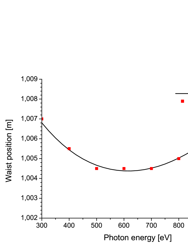
Figure 53: Focusing at the slit position. Variation of the focus location as a function photon energy.

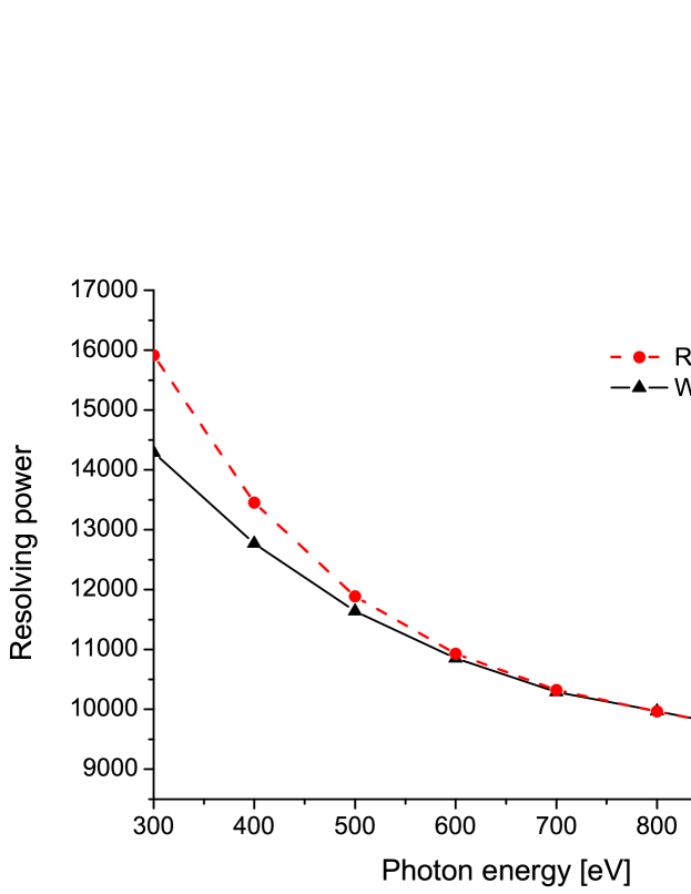
Figure 54: Resolving power of the grating monochromator at closed slit, as a function of the photon energy. Squares are calculated using wave optics and including aberrations, and circles are calculated with ray-tracing code.

The optical system was simulated using the ray-tracing code SHADOW SHAD in order to evaluate the performance of the monochromator. The reason for modeling the monochromator using ray-tracing is the need to check the results found by wave optics calculations, especially minimization of aberrations. The source has been modeled as a Gaussian-shaped beam and with Gaussian divergence distribution as a function of wavelength, since the XFEL source will be nearly transform-limited. We performed ray-tracing simulations at three different photon energies, $1000.2$ eV, $1000.0$ eV and $999.8$ eV. We assumed the rms value of $17.1~{}\mu$m for the source size, and $5.57~{}\mu$rad for the beam divergence. No figure errors (i.e. no slope errors) were included. In this way, the FEL source has been propagated over grating and exit slit, and then over the refocusing mirror. Ray-tracing results at the plane of the exit slit for photons of $1000.2$ eV, $1000.0$ eV, and $999.8$ eV (when the monochromator is tuned to $1000$ eV) are shown in Fig.49. The histograms show that in the dispersive (tangential) and non-dispersive (sagittal) direction the distribution is almost Gaussian. As it can be seen from the figure, the focusing properties of the monochromator at this photon energy are excellent, and resolution is larger than $5000$. The corresponding ray-tracing results for $0.5$ keV photons are shown in Fig. 50. The figure shows that the same focusing quality is obtained also in this case. Actually, this is the case for all photon energies in the range between $0.3$ keV and $1$ keV due to the VLS toroidal grating parameters, minimizing defocusing and coma aberrations. Fig. 51 and Fig. 52 display results of ray-tracing simulations at the entrance of the second undulator.

The location of the beam focus, shown in Fig. 53, was found to vary with the energy around the slit. Fig. 53 also shows a comparison between results found with ray tracing and wave optics calculations. Fig. 54 summarizes the energy resolution obtained from the linear dispersion and the FWHM of the spot size at the exit slit plane as a function of the photon energy. Comparing to the optimal slit distance found by wave optics calculations, it is seen that there is a very good agreement between coherent and incoherent models. However a complete, straightforward analysis of the full self-seeding monochromator setup can be only be performed in terms of wave optics.

4.8 Heat load

Table 2: Heat load on the grating

	Units
Photon energy	keV	0.8
Incident power	W	4.5
Absorbed power	W	1.4
Footprint	cm2	0.02
Power density	W/mm2	0.7

Figure 55: Total reflectivity of the grating as a function of photon energy.

X-ray optics can survive the high average power during one macropulse from the European XFEL. The heat load can be evaluated by considering the absorbed power on the grating. In table 2 we consider the case for an electron beam with 0.1 nC charge. The power absorbed by the grating can be evaluated by taking into account the parameters of the first undulator source (see section 5 and Fig. 58) and the total reflectivity of the grating, Fig. 55. The results presented here refer to the case of an impinging pulse train composed by $2700$ FEL pulses of $0.001$ mJ each, at the photon energy of $800$ eV. The power is averaged over the $0.6$ ms of the pulse train, which is the most extreme approximation. A similar power density, $0.6$ W/mm²- $1.3$ W/mm² absorbed in the grating has been reported in previous studies for the European XFEL TRAN .

4.9 Single shot damage

While the average absorbed power on the grating power is still moderate, the peak power within the single pulse from the first SASE undulator will be in the range of a fraction of GW. At these power levels, the main issue may be no longer related with thermal distortion, but rather with the possibility of ablation of the grating surface, which would result in permanent damage. Ablation depends on the radiation dose per pulse, which can be quantified as the energy absorbed in the volume defined by the projected beam area on the optical element and by one attenuation length, which is the depth into the material, measured along the surface normal, where the radiation intensity falls to $2,72$ times of its value at the surface. Normalized to one atom this energy corresponds to the atomic dose near the surface XTDR

$$D=\frac{E_{\mathrm{pulse}}(1-R)\theta_{i}}{2\pi\sigma^{2}l_{\mathrm{att}}n_{A}}~{},$$ (185)

where $E_{\mathrm{pulse}}$ is the energy in one radiation pulse, $R$ is the reflectivity, $l_{\mathrm{att}}$ is the attenuation length, $\sigma$ is the rms of the Gaussian beam intensity distribution immediately in front of the grating, and $n_{A}$ denotes the element-specific density of atoms. For Pt coating we find $n_{A}\sim 6.4\cdot 10^{22}$ cm^-3, $R\sim 0.7$, $l_{\mathrm{att}}\sim 2$ nm, $\sigma\sim 0.05$ mm, and $E_{\mathrm{pulse}}\sim 0.001$ mJ. The calculated dose reaches up to $15$ meV/atom. This is about $30$ times below the melting threshold for Pt FENG2 . The grating is therefore safe from damage.

5 FEL simulations

With reference to Fig. 1, we performed a feasibility study with the help of the FEL code Genesis 1.3 GENE running on a parallel machine. We will present a feasibility study for the SASE3 FEL line of the European XFEL, based on a statistical analysis consisting of $100$ runs. The overall beam parameters used in the simulations are presented in Table 3.

Table 3: Parameters for the mode of operation at the European XFEL used in this paper.

	Units
Undulator period	mm	68
Periods per cell	-	73
Total number of cells	-	21
Intersection length	m	1.1
Energy	GeV	10.5
Charge	nC	0.1

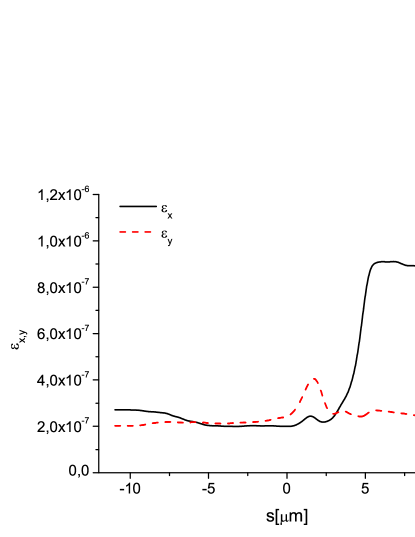
Figure 56: Results from electron beam start-to-end simulations at the entrance of SASE3. (First Row, Left) Current profile. (First Row, Right) Normalized emittance as a function of the position inside the electron beam. (Second Row, Left) Energy profile along the beam. (Second Row, Right) Electron beam energy spread profile. (Bottom row) Resistive wakefields in the SASE3 undulator.

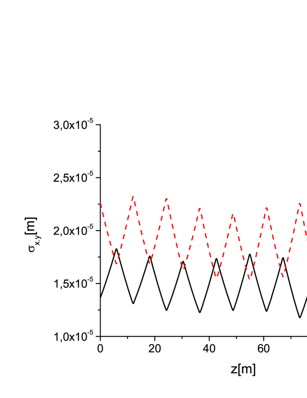
Figure 57: Evolution of the horizontal and vertical dimensions of the electron bunch as a function of the distance inside the SASE3 undulator. The plots refer to the longitudinal position inside the bunch corresponding to the maximum current vale.

The expected beam parameters at the entrance of the SASE3 undulator, and the resistive wake inside the undulator are shown in Fig. 56, S2ER . The evolution of the transverse electron bunch dimensions are plotted in Fig. 57.

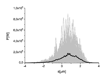
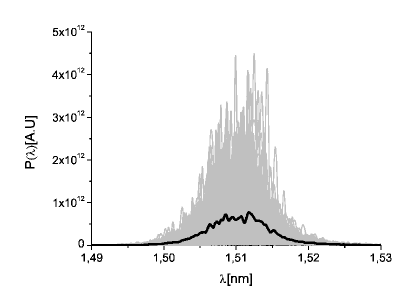
Figure 58: Power distribution and spectrum of the X-ray radiation pulse after the first undulator. Grey lines refer to single shot realizations, the black line refers to the average over a hundred realizations.

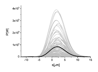
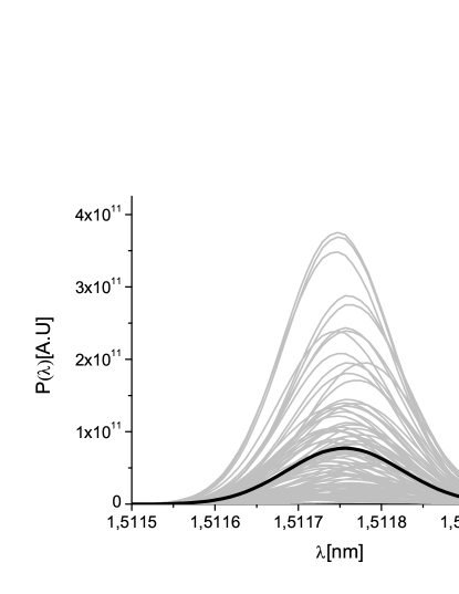
Figure 59: Power distribution and spectrum of the X-ray radiation pulse after the monochromator. This pulse is used to seed the electron bunch at the entrance of the output undulator. Grey lines refer to single shot realizations, the black line refers to the average over a hundred realizations.

The SASE pulse power and spectrum after the first undulator is shown in Fig. 58. This pulse goes through the grating monochromator. The monochromator lineshape is presented in Fig. 10. At the exit of the monochromator, one obtains the seed pulse, Fig. 59. As explained before, the monochromator introduces only a short optical delay of about $0.7$ ps, which can be easily compensated by the electron chicane. The chicane also washes out the electron beam microbunching. As a result, at the entrance of the second (output) undulator the electron beam and the radiation pulse can be recombined.

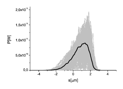
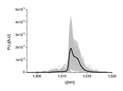
Figure 60: Power distribution and spectrum of the X-ray radiation pulse after the second undulator in the untapered case. Grey lines refer to single shot realizations, the black line refers to the average over a hundred realizations.

Figure 61: Evolution of the energy per pulse and of the energy fluctuations as a function of the undulator length in the untapered case. Grey lines refer to single shot realizations, the black line refers to the average over a hundred realizations.

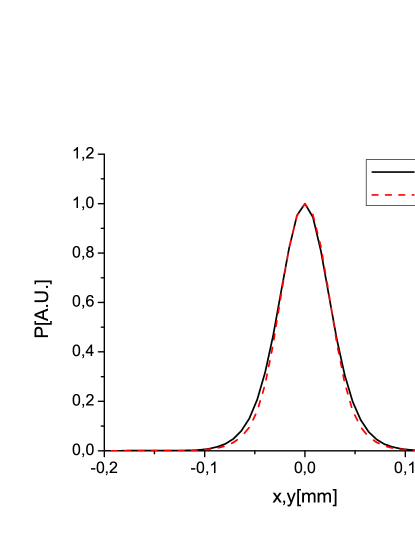
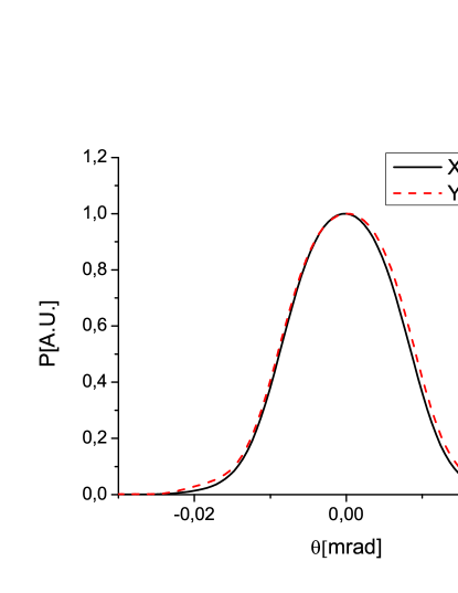
Figure 62: (Left plot) Transverse radiation distribution in the untapered case at the exit of the output undulator. (Right plot) Directivity diagram of the radiation distribution in the case of tapering at the exit of the output undulator.

If the output undulator is not tapered, one needs $7$ sections to reach saturation. The best compromise between power and spectral bandwidth are reached after $6$ sections, Fig. 60. In this case, the evolution of the energy per pulse and of the energy fluctuations as a function of the undulator length are shown in Fig. 61. The pulse now reaches the $100$ GW power level, with an average relative FWHM spectral width narrower than $10^{-3}$. Finally, the transverse radiation distribution and divergence at the exit of the output undulator are shown in Fig. 62.

Figure 63: Taper configuration for high-power mode of operation at $1.5$ nm.

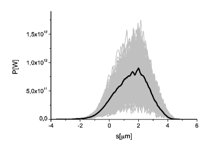
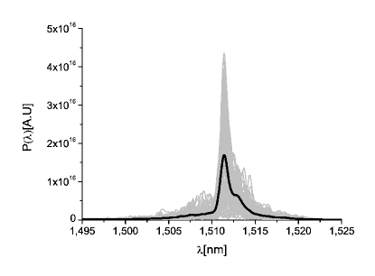
Figure 64: Power distribution and spectrum of the X-ray radiation pulse after the second undulator in the tapered case. Grey lines refer to single shot realizations, the black line refers to the average over a hundred realizations.

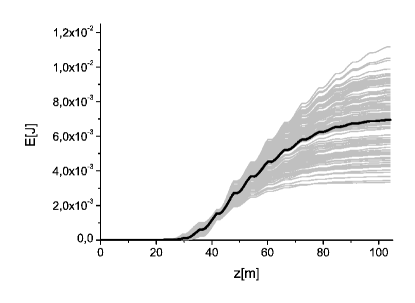
Figure 65: Evolution of the energy per pulse and of the energy fluctuations as a function of the undulator length in the tapered case. Grey lines refer to single shot realizations, the black line refers to the average over a hundred realizations.

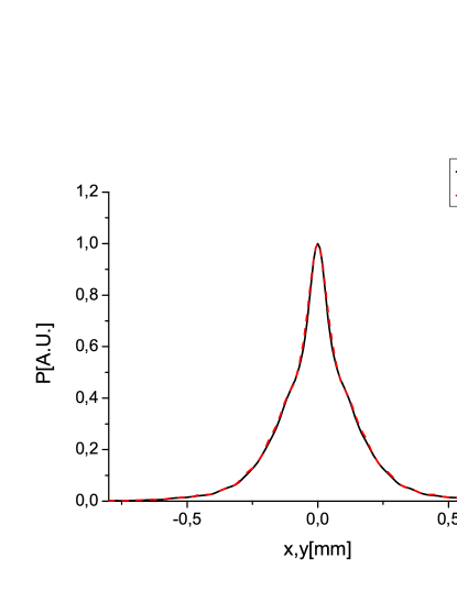
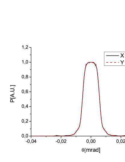
Figure 66: (Left plot) Transverse radiation distribution in the case of tapering at the exit of the output undulator. (Right plot) Directivity diagram of the radiation distribution in the case of tapering at the exit of the output undulator.

The most promising way to increase the output power is via post-saturation tapering. Tapering consists in a slow reduction of the field strength of the undulator in order to preserve the resonance wavelength, while the kinetic energy of the electrons decreases due to the FEL process. The undulator taper could be simply implemented as a step taper from one undulator segment to the next, as shown in Fig. 63. The magnetic field tapering is provided by changing the undulator gap. A further increase in power is achievable by starting the FEL process from the monochromatic seed, rather than from noise. The reason is the higher degree of coherence of the radiation in the seed case, thus involving, with tapering, a larger portion of the bunch in the energy-wavelength synchronism. Using the tapering configuration in Fig. 63, one obtains the output characteristics, in terms of power and spectrum, shown in Fig. 64. The output power is increased of about a factor ten, allowing one to reach about one TW. The spectral width remains almost unvaried, with an average relative bandwidth (FWHM) narrower than $10^{-3}$. The evolution of the energy per pulse and of the energy fluctuations as a function of the undulator length are shown in Fig. 61. The transverse radiation distribution and divergence at the exit of the output undulator are shown in Fig. 66. By comparison with Fig. 62 one can see that the divergence decrease is accompanied by an increase in the transverse size of the radiation spot at the exit of the undulator.

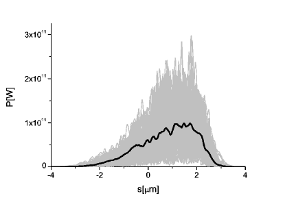
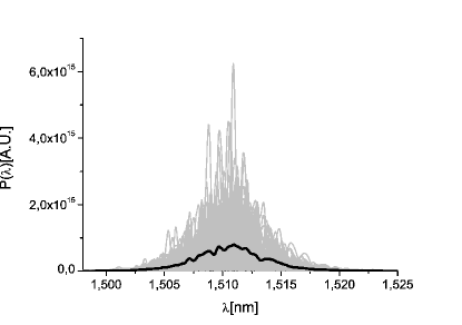
Figure 67: Power distribution and spectrum of the baseline SASE X-ray radiation pulse at saturation. Grey lines refer to single shot realizations, the black line refers to the average over a hundred realizations.

Figure 68: Evolution of the energy per pulse and of the energy fluctuations as a function of the undulator length in the case of the baseline SASE pulse. Grey lines refer to single shot realizations, the black line refers to the average over a hundred realizations.

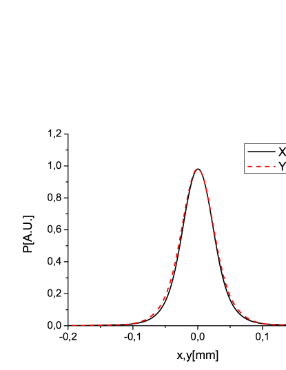
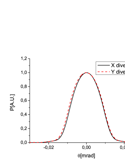
Figure 69: (Left plot) Transverse radiation distribution in the case of the baseline SASE pulse at saturation. (Right plot) Directivity diagram of the radiation distribution in the case of the baseline SASE pulse at saturation.

Finally, it is interesting to compare the results for the self-seeded beam with the characteristics of the SASE pulse at SASE3 generated with the same electron beam. The output SASE characteristics at saturation, in terms of power and spectrum, shown in Fig. 67. The evolution of the energy in the SASE pulse and of the energy fluctuations as a function of the undulator length are shown in Fig. 68. The transverse radiation distribution and divergence at saturation are shown in Fig. 69.

6 Conclusions

Historically, self-seeding methods were first proposed for the soft X-ray region, and were based on the use of grating monochromators SELF , STTF . However, self-seeding techniques were first successfuly demonstrated in the hard X-ray region at the LCLS EMNAT , based on the use of a crystal monochromator. The working principle for such monochromator was invented in OURLB , and resulted into a very compact self-seeding setup design fitting within a single undulator module. During the last three years, significant efforts were dedicated to both theoretical investigation and $R\&D$ at the LCLS, leading to the design of a compact self-seeding setup in the soft X-ray range, based on a grating monochromator. The evolution of the design can be reconstructed from FENG -FENG3 , striving at the same time for the needed resolution and compactness. The development of a self-seeding grating monochromator with the same compactness of a single-crystal monochromator is a challenging problem. However, the final design of the LCLS soft X-ray self-seeding setup has many advantages. It is very compact and fits within one undulator module. It is very simple and includes only four optical elements. It does not include an entrance slit and during discussions, authors of FENG3 pointed that this design might be operated even without exit slit by using the electron beam and the spatial dispersion at the second undulator entrance for spectral filtering purpose.

In this article we present a technical study for a soft x-ray self-seeding setup at the European XFEL. In particular we focus on design and performance of a very compact self-seeding grating monochromator, based on the LCLS design, which has been adapted to the needs of the European XFEL. Usually, soft X-ray monochromators operate with incoherent sources and their design is based on the use of ray-tracing codes. However, XFEL beams are almost completely transversely coherent, and in our case the optical system was studied using a wave optics method in combination with FEL simulations to evaluate the performance of the self-seeding scheme. Our wave optics analysis takes into account the actual FEL beam wavefront, third order aberrations and surface errors from each optical elements. Wave optics together with FEL simulations are naturally applicable to the study the influence of finite slit size on the seeding efficiency. Most results presented in FENG3 were obtained in the framework of a Gaussian beam model, in combination with ray-tracing for Gaussian ray distribution. This is a very fruitful approach, allowing one for studying many features of the self-seeding monochromator by means of relatively simple tools. Using our approach, we give a quantitative answer to the question of the accuracy of the Gaussian beam model. It is also important to quantitatively analyze the filtering process without exit slit. Wave optics in combination with FEL simulations is the only method available to this aim. We conclude that the mode of operation without slit is superior to the conventional mode of operation, and a finite slit size would only lead to a reduction of the monochromator performance. We therefore propose an optimized design based on a toroidal VLS grating and three mirrors, without exit slit. The monochromator covers the range between $300$ eV and $1000$ eV, with a resolution never falling below $7000$, and introduces a photon delay of only $0.7$ ps. This allows the entire self-seeding setup to be fit into a single $5$ m-long undulator segment. The overall performance of the setup is studied with the help of FEL simulations, which show that, in combination with post-saturation tapering, the SASE3 baseline at the European XFEL could deliver TW-class, nearly Fourier-limited radiation pulses in the soft X-ray range. Although we explicitly studied the a soft x-ray self-seeding setup for the SASE3 undulator baseline at the European XFEL, the same setup can be used without modifications also for the dedicated bio-imaging beamline, a concept that was proposed in BIO1 -BIO3 as a possible future upgrade of the European XFEL. By exploiting third harmonic generation and fresh bunch technique together with the self-seeding mode of operation BZVI -WU one can extend the operation of the soft x-ray self-seeding setup to the range between $1$ keV up to $3$ keV, thus covering the sulfur K-edge without changes in the grating monochromator design BIO3 . The X-ray beam will thus be delivered in ultrashort pulses with 1 TW peak power within the extended photon energy range between 0.3 keV up to 3 keV. For operation at higher photon energies x-ray self-seeding setups based on single crystal monochromators can be used.

7 Acknowledgements

We thank Daniele Cocco, Paul Emma, Yiping Feng, Jerome Hastings, Philip Heimann and Jacek Krzywinski for useful discussions. We are grateful to Massimo Altarelli, Reinhard Brinkmann, Henry Chapman, Janos Hajdu, Viktor Lamzin, Serguei Molodtsov and Edgar Weckert for their support and their interest during the compilation of this work.

References

- [1] J. Feldhaus et al., Optics. Comm. 140, 341 (1997).
- [2] E. Saldin, E. Schneidmiller, Yu. Shvyd’ko and M. Yurkov, NIM A 475 357 (2001).
- [3] E. Saldin, E. Schneidmiller and M. Yurkov, NIM A 445 178 (2000).
- [4] R. Treusch, W. Brefeld, J. Feldhaus and U Hahn, Ann. report 2001 ”The seeding project for the FEL in TTF phase II” (2001).
- [5] A. Marinelli et al., Comparison of HGHG and Self Seeded Scheme for the Production of Narrow Bandwidth FEL Radiation, Proceedings of FEL 2008, MOPPH009, Gyeongju (2008).
- [6] G. Geloni, V. Kocharyan and E. Saldin, ”Scheme for generation of highly monochromatic X-rays from a baseline XFEL undulator”, DESY 10-033 (2010).
- [7] Y. Ding, Z. Huang and R. Ruth, Phys.Rev.ST Accel.Beams, vol. 13, p. 060703 (2010).
- [8] G. Geloni, V. Kocharyan and E. Saldin, ”A simple method for controlling the line width of SASE X-ray FELs ”, DESY 10-053 (2010).
- [9] Geloni, G., Kocharyan, V., and Saldin, E., ”Cost-effective way to enhance the capabilities of the LCLS baseline”, DESY 10-133 (2010).
- [10] Geloni, G., Kocharyan V., and Saldin, E., ”A novel Self-seeding scheme for hard X-ray FELs”, Journal of Modern Optics, vol. 58, issue 16, pp. 1391-1403, DOI:10.1080/09500340.2011.586473 (2011).
- [11] J. Amann et al., Nature Photonics, DOI:10.1038/NPHOTON.2012.180 (2012).
- [12] Y. Feng, J. Hastings, P. Heimann, M. Rowen, J. Krzywinski, and J. Wu, ”X-ray Optics for soft X-ray self-seeding the LCLS-II”, proceedings of 2010 FEL conference, Malmo, Sweden, (2010).
- [13] Y. Feng, P. Heimann, J. Wu, J. Krzywinski, M. Rowen, and J. Hastings, ”Compact Grating Monochromator Design for LCLS-I Soft X-ray Self-Seeding”, https://slacportal.slac.stanford.edu/ sites/lclspublic/lclsii/Lists/LCLSII Calendar/PhysicsMeetings.aspx, May 2011 and https://sites.google.com/a/lbl.gov/realizing-the-potential-of-seeded-fels-in-the-soft-x-ray-regime-workshop/talks, October 2011
- [14] Y. Feng et al., ”System design for self-seeding the LCLS at soft X-ray energies”, to appear in the Proceedings of the 24th International FEL Conference, Nara, Japan (2012).
- [15] A. Lin and J.M. Dawson, Phys. Rev. Lett. 42 2172 (1986)
- [16] P. Sprangle, C.M. Tang and W.M. Manheimer, Phys. Rev. Lett. 43 1932 (1979)
- [17] N.M. Kroll, P. Morton and M.N. Rosenbluth, IEEE J. Quantum Electron., QE-17, 1436 (1981)
- [18] T.J. Orzechovski et al., Phys. Rev. Lett. 57, 2172 (1986)
- [19] W. Fawley et al., NIM A 483 (2002) p 537
- [20] M. Cornacchia et al., J. Synchrotron rad. (2004) 11, 227-238
- [21] X. Wang et al., PRL 103, 154801 (2009)
- [22] G. Geloni, V. Kocharyan and E. Saldin, ”Scheme for generation of fully coherent, TW power level hard x-ray pulses from baseline undulators at the European XFEL”, DESY 10-108 (2010).
- [23] Geloni, G., Kocharyan, V., and Saldin, E., ”Production of transform-limited X-ray pulses through self-seeding at the European X-ray FEL”, DESY 11-165 (2011).
- [24] W.M. Fawley et al., Toward TW-level LCLS radiation pulses, TUOA4, to appear in the FEL 2011 Conference proceedings, Shanghai, China, 2011
- [25] J. Wu et al., Simulation of the Hard X-ray Self-seeding FEL at LCLS, MOPB09, to appear in the FEL 2011 Conference proceedings, Shanghai, China, 2011
- [26] Y. Jiao et al. Phys. Rev. ST Accel. Beams 15, 050704 (2012)
- [27] I. Zagorodnov, ”Beam Dynamics simulations for XFEL”, http://www.dedy.de/sfel-beam/s2e (2011).
- [28] G. Geloni, V. Kocharyan and E. Saldin, ”Conceptual design of an undulator system for a dedicated bio-imaging beamline at the European X-ray FEL”, DESY 12-082, http://arxiv.org/abs/1205.6345 (2012).
- [29] G. Geloni, V. Kocharyan and E. Saldin, ”Optimization of a dedicated bio-imaging beamline at the European X-ray FEL”, DESY 12-159, http://arxiv.org/abs/1209.5972 (2012).
- [30] C. Svetina, M. Zagrando, A. Bianco and D. Cocco, ”A Fixed including angle monochromator for the 4th generation light source FERMI@ELETRA”, Proc. of SPIE Vol. 7448, 74480.2009 (2009).
- [31] M. Roper Nucl. Instruments and Methods in Physics Research A 635 580-587 (2011).
- [32] J. Hajdu, Curr. Opin. Struct. Biol. 10, 569 (2000)
- [33] R. Neutze et al., Nature 406, 752 (2000)
- [34] K. J. Gaffney and H. N. Chapman, Science 316, 1444 (2007)
- [35] M. M. Seibert et al., Nature 470 (7332) 78-81 (2011)
- [36] S. Baradaran et al., LCLS-II New Instruments Workshops Report, SLAC-R-993 (2012), see Section 4.3.2. by H. Chapman et al., and Section 4.3.3. by F. R. N. C. Maia et al.
- [37] S. Reiche et al., Nucl. Instr. and Meth. A 429, 243 (1999).
- [38] S. Self, Applied Optics 22, 5 (1983).
- [39] D. Marcuse, ”Light transmission optics”, Van Nostrand Reinhold Company, New York (1982).
- [40] G. P. Agarwal ”Nonlinear Fiber optics” Academic Press, New York (1989).
- [41] Ting-Chung Poon and Taegeun Kim, ”Engineering Optcs with Matlab”, World Scientific Publishing Co. Pte. Ltd. (2006).
- [42] G. Stroke, ”An Introduction to Coherent Optics and Holography”, Academic Press (1966).
- [43] R. Petit and L. Botten. ”Electromagnetic Theory of Grating” Springer-Verlag (1980)
- [44] M. Boots, D. Muir and A. Moeves, J. Synchrotron Rad. 20, 272-285 (2013).
- [45] M. Itou, T. Harada, and T. Kita, Applied Optics 28, 1 (1989).
- [46] I. Moreno, et al., European Journal of Physics 26, 261-271 (2005).
- [47] A. E. Siegman, J. Opt. Soc. Am. A 2, 1793 (1985).
- [48] A. April, and N. McCarthy, Optics Communications 271, 327-331 (2007).
- [49] R. J. Thomas, Proc. SPIE 4853, 411-418 (2002).
- [50] H. Haber, J. Opt. Soc. Am. 40, 153 (1950).
- [51] T. Harada et al., Applied optics 37, 28, 6803-6810 (1998)
- [52] http://www.henke.lbl.gov/opticalconstants/
- [53] http://www.gsolver.com
- [54] A. Barty et al., Optics Express 17, 15508 (2009).
- [55] P. Heimann et al., Review of Scientific Instruments 82, 093104 (2011).
- [56] http://www.esrf.eu/computing/scientific/raytracing/
- [57] H. Sinn et al., ”Conceptual design report: X-ray optics and Beam Transport”, XFEL EU TR-2011-002 (2011).
- [58] M. Altarelli, et al. (Eds.) XFEL, The European X-ray Free-Electron Laser, Technical Design Report, DESY 2006-097, Hamburg (2006).
- [59] I Ben-Zvi and L. H. Yu, Nucl. Instr. and Methods, A 393, 96 (1997).
- [60] G. Geloni, V. Kocharyan and E. Saldin, ”A simple method for controlling the line width of SASE X-ray FELs”, DESY 10-053 (2010).
- [61] J. Wu et al., ”Staged self-seeding scheme for narrow bandwidth , ultra-short X-ray harmonic generation free electron laser at LCLS”, proceedings of 2010 FEL conference, Malmo, Sweden, (2010).